Ridge Type Shrinkage Estimation of Seemingly Unrelated Regressions And Analytics of Economic and Financial Data from “Fragile Five” Countries

Abstract

In this paper, we suggest improved estimation strategies based on preliminarily test and shrinkage principles in a seemingly unrelated regression model when explanatory variables are affected by multicollinearity. To that end, we split the vector regression coefficient of each equation into two parts: one includes the coefficient vector for the main effects, and the other is a vector for nuisance effects, which could be close to zero. Therefore, two competing models per equation of the system regression model are obtained: one includes all the regression of coefficients (full model); the other (sub model) includes only the coefficients of the main effects based on the auxiliary information. The preliminarily test estimation improves the estimation procedure if there is evidence that the vector of nuisance parameters does not provide a useful contribution to the model. The shrinkage estimation method shrinks the full model estimator in the direction of the sub-model estimator. We conduct a Monte Carlo simulation study in order to examine the relative performance of the suggested estimation strategies. More importantly, we apply our methodology based on the preliminarily test and the shrinkage estimations to analyse economic data by investigating the relationship between foreign direct investment and several economic variables in the “Fragile Five” countries between 1983 and 2018.

1. Introduction

A seemingly unrelated regression (SUR) system, originally proposed by Zellner (1962), comprises multiple individual regression equations that are correlated with each other. Zellner’s idea was to improve estimation efficiency by combining several equations into a single system. Contrary to SUR estimation, the ordinary least squares (OLS) estimation loses its efficiency and will not produce best linear unbiased estimates (BLUE) when the error terms between the equations in the system are correlated. This method has a wide range of applications in economic and financial data and other similar areas (Shukur 2002; Srivastava and Giles 1987; Zellner 1962). For example, Dincer and Wang (2011) investigated the effects of ethnic diversity on economic growth. Williams (2013) studied the effects of financial crises on banks. Since it considers multiple related equations simultaneously, a generalized least squares (GLS) estimator is used to take into account the effect of errors in these equations. Barari and Kundu (2019) reexamined the role of the Federal Reserve in triggering the recent housing crisis with a vector autoregression (VAR) model, which is a special case of the SUR model with lagged variables and deterministic terms as common regressors. One might also consider the correlations of explanatory variables in SUR models. Alkhamisi and Shukur (2008) and Zeebari et al. (2012, 2018) considered a modified version of the ridge estimation proposed by Hoerl and Kennard (1970) for these models. Alkhamisi (2010) proposed two SUR-type estimators by combining the SUR ridge regression and the restricted least squares methods. These recent studies demonstrated that the ridge SUR estimation is superior to classical estimation methods in the presence of multicollinearity. Srivastava and Wan (2002) considered the Stein-rule estimators from James and Stein (1961) in SUR models with two equations.

In our study, we consider preliminarily test and shrinkage estimation, more information on which can be found in Ahmed (2014), in ridge-type SUR models when the explanatory variables are affected by multicollinearity. In a previous paper, we combined penalized estimations in an optimal way to define shrinkage estimation (Ahmed and Yüzbaşı 2016). Gao et al. (2017) suggested the use of the weighted ridge regression model for post-selection shrinkage estimation. Yüzbaşı et al. (2020) gave detailed information about generalized ridge regression for a number of shrinkage estimation methods. Srivastava and Wan (2002) and Arashi and Roozbeh (2015) considered Stein-rule estimation for SUR models. Erdugan and Akdeniz (2016) proposed a restricted feasible SUR estimate of the regression coefficients.

The organization of this paper is as follows: In Section 2, we briefly review the SUR model and some estimation techniques, including the ridge type. In Section 3, we introduce our new estimation methodology. A Monte Carlo simulation is conducted in Section 4, and our economic data are analysed in Section 5. Finally, some concluding remarks are given in Section 6.

2. Methodology

Consider the following model:

$${\mathbf{Y}}_i={\mathbf{X}}_i{\mathbf{\beta }}_i+{\mathbf{\epsilon }}_i,i=1,2,\cdots ,M,$$

(1)

the $i^{\mathrm{th}}$ equation of an M seemingly unrelated regression equation with T number of observations per equation. ${\mathbf{Y}}_i$ is a $T\times 1$ vector of T observations; ${\mathbf{X}}_i$ is a $T\times p_i$ full column rank matrix of T observations on $p_i$ regressors; and ${\mathbf{\beta }}_i$ is a $p_i\times 1$ vector of unknown parameters.

Equation (1) can be rewritten as follows:

$$\mathbf{Y}=\mathbf{X}\mathbf{\beta }+\mathbf{\epsilon },$$

(2)

where $\mathbf{Y}={\left({\mathbf{Y}}_1^{\prime },{\mathbf{Y}}_2^{\prime },\cdots ,{\mathbf{Y}}_M^{\prime }\right)}^{\prime }$ is the vector of responses and $\mathbf{\epsilon }={\left({\mathbf{\epsilon }}_1^{\prime },{\mathbf{\epsilon }}_2^{\prime },\cdots ,{\mathbf{\epsilon }}_M^{\prime }\right)}^{\prime }$ is the vector of disturbances with dimension $TM\times 1$, $\mathbf{X}=diag\left({\mathbf{X}}_1,{\mathbf{X}}_2,\cdots ,{\mathbf{X}}_M\right)$ of dimension $TM\times p$, and $\mathbf{\beta }={\left({\mathbf{\beta }}_1^{\prime },{\mathbf{\beta }}_2^{\prime },\cdots ,{\mathbf{\beta }}_M^{\prime }\right)}^{\prime }$ of dimension $p\times 1$, for $p={\sum }_{i=1}^M{p}_i$.

The disturbances vector $\mathbf{\epsilon }$ satisfies the properties:

$$E(\mathbf{\epsilon })=\mathbf{0}$$

and:

$$E(\mathbf{\epsilon }{\mathbf{\epsilon }}^{\prime })=\left[\begin{array}{ccc}{\sigma }_{11}\mathbf{I}& \cdots & {\sigma }_{1M}\mathbf{I}\\ ⋮& \ddots & \\ {\sigma }_{M1}\mathbf{I}& \cdots & {\sigma }_{MM}\mathbf{I}\end{array}\right]=\mathsf{\Sigma }\otimes \mathbf{I},$$

where $\mathsf{\Sigma }=\left[{\sigma }_{ij}\right],i,j=1,2,\cdots ,M$ is an $M\times M$ positive definite symmetric matrix, ⊗ stands for the Kronecker product, and $\mathbf{I}$ is an identity matrix of order of $T\times T$. Following Greene (2019), we assume strict exogeneity of ${\mathbf{X}}_i$,

$$E\left[\mathbf{\epsilon }|{\mathbf{X}}_1,{\mathbf{X}}_2,\cdots ,{\mathbf{X}}_M\right]=\mathbf{0},$$

and homoscedasticity:

$$E\left[{\mathbf{\epsilon }}_i{\mathbf{\epsilon }}_i^{\prime }|{\mathbf{X}}_1,{\mathbf{X}}_2,\cdots ,{\mathbf{X}}_M\right]={\sigma }_{ii}\mathbf{I}.$$

Therefore, it is assumed that disturbances are uncorrelated across observations, that is,

$$E\left[{\mathbf{\epsilon }}_{it}{\mathbf{\epsilon }}_{js}|{\mathbf{X}}_1,{\mathbf{X}}_2,\cdots ,{\mathbf{X}}_M\right]={\sigma }_{ij},\mathrm{if}t=s\mathrm{and}0\mathrm{otherwise},$$

and it is assumed that disturbances are correlated across equations, that is,

$$E\left[{\mathbf{\epsilon }}_i{\mathbf{\epsilon }}_j^{\prime }|{\mathbf{X}}_1,{\mathbf{X}}_2,\cdots ,{\mathbf{X}}_M\right]={\sigma }_{ij}\mathbf{I}.$$

The OLS and GLS estimator of model (2) are thus given as:

$${\widehat{\mathbf{\beta }}}^{\mathrm{OLS}}={({\mathbf{X}}^{\prime }\mathbf{X})}^{-1}{\mathbf{X}}^{\prime }\mathbf{Y}$$

and:

$${\widehat{\mathbf{\beta }}}^{\mathrm{GLS}}={({\mathbf{X}}^{\prime }({\mathsf{\Sigma }}^{-1}\otimes \mathbf{I})\mathbf{X})}^{-1}{\mathbf{X}}^{\prime }({\mathsf{\Sigma }}^{-1}\otimes \mathbf{I})\mathbf{Y}.$$

${\widehat{\mathbf{\beta }}}^{\mathrm{OLS}}$ simply consists of the OLS estimators computed separately from each equation and omits the correlations between equation, as can be seen in Kuan (2004). Hence, it should use the GLS estimator when correlations exist among equations. However, the true covariance matrix $\mathsf{\Sigma }$ is generally unknown. The solution for this problem is a feasible generalized least squares (FGLS) estimation, which uses covariance matrix $\widehat{\mathsf{\Sigma }}$ of $\mathsf{\Sigma }$ in the estimation of GLS. In many cases, the residual covariance matrix is calculated by:

$${\sigma }_{ij}=\frac{{\widehat{\mathbf{\epsilon }}}_i^{\prime }{\widehat{\mathbf{\epsilon }}}_j}{T-max(p_i,p_j)},i,j=1,\cdots ,M,$$

where ${\widehat{\mathbf{\epsilon }}}_i={\mathbf{Y}}_i-{\mathbf{X}}_i{\widehat{\mathbf{\beta }}}_i$ represents residuals from the $i^{\mathrm{th}}$ equation and ${\widehat{\mathbf{\beta }}}_i$ may be the OLS or ridge regression (RR) estimation such that ${({\mathbf{X}}_i^{\prime }{\mathbf{X}}_i+\lambda \mathbf{I})}^{-1}{\mathbf{X}}_i^{\prime }{\mathbf{Y}}_i$ with the tuning parameter $\lambda \ge 0$. Note that we use the RR solution to estimate $\mathsf{\Sigma }$ in our numerical studies because we assume that two or more explanatory variables in each equation are linearly related. Therefore, $\widehat{\mathsf{\Omega }}=\widehat{\mathsf{\Sigma }}\otimes \mathbf{I}$, the FGLS of the SUR system, is:

$${\widehat{\mathbf{\beta }}}^{\mathrm{FGLS}}={({\mathbf{X}}^{\prime }{\widehat{\mathsf{\Omega }}}^{-1}\mathbf{X})}^{-1}{\mathbf{X}}^{\prime }{\widehat{\mathsf{\Omega }}}^{-1}\mathbf{Y}.$$

By following Srivastava and Giles (1987) and Zeebari et al. (2012), we first transform Equation (2) by using the following transformations, in order to retain the information included in the correlation matrix of cross equation errors:

$${\mathbf{Y}}_{\ast }=\left({\widehat{\mathsf{\Sigma }}}^{-1/2}\otimes \mathbf{I}\right)\mathbf{Y},{\mathbf{X}}_{\ast }=\left({\widehat{\mathsf{\Sigma }}}^{-1/2}\otimes \mathbf{I}\right)\mathbf{X}\mathrm{and}{\mathbf{\epsilon }}_{\ast }=\left({\widehat{\mathsf{\Sigma }}}^{-1/2}\otimes \mathbf{I}\right)\mathbf{\epsilon }.$$

Hence, Model (2) turns into:

$${\mathbf{Y}}_{\ast }={\mathbf{X}}_{\ast }\mathbf{\beta }+{\mathbf{\epsilon }}_{\ast }.$$

(3)

The spectral decomposition of the symmetric matrix ${\mathbf{X}}_{\ast }^{\prime }{\mathbf{X}}_{\ast }$ is ${\mathbf{X}}_{\ast }^{\prime }{\mathbf{X}}_{\ast }=\mathbf{P}\mathsf{\Lambda }{\mathbf{P}}^{\prime }$ with $\mathbf{P}{\mathbf{P}}^{\prime }=\mathbf{I}$. Model (3) can then be written as:

$$\begin{array}{ccc}\hfill {\mathbf{Y}}_{\ast }& =& {\mathbf{X}}_{\ast }\mathbf{P}{\mathbf{P}}^{\prime }\mathbf{\beta }+{\mathbf{\epsilon }}_{\ast }\hfill \\ & =& \mathbf{Z}\mathbf{\alpha }+{\mathbf{\epsilon }}_{\ast },\hfill \end{array}$$

(4)

with $\mathbf{Z}={\mathbf{X}}_{\ast }\mathbf{P}$, $\mathbf{\alpha }={\mathbf{P}}^{\prime }\mathbf{\beta }$ and ${\mathbf{Z}}^{\prime }\mathbf{Z}={\mathbf{P}}^{\prime }{\mathbf{X}}_{\ast }^{\prime }{\mathbf{X}}_{\ast }\mathbf{P}=\mathsf{\Lambda }$, so that $\mathsf{\Lambda }$ is a diagonal matrix of eigenvalues and $\mathbf{P}$ is a matrix whose columns are eigenvectors of ${\mathbf{X}}_{\ast }^{\prime }{\mathbf{X}}_{\ast }$.

The OLS estimator of model (4) is:

$${\widehat{\mathbf{\alpha }}}^{\mathrm{OLS}}={({\mathbf{Z}}^{\prime }\mathbf{Z})}^{-1}{\mathbf{Z}}^{\prime }{\mathbf{Y}}_{\ast }.$$

The least squares estimates of $\mathbf{\beta }$ in model (2) can be obtained by an inverse linear transformation as:

$${\widehat{\mathbf{\beta }}}^{\mathrm{OLS}}={({\mathbf{P}}^{\prime })}^{-1}{\widehat{\mathbf{\alpha }}}^{\mathrm{OLS}}=\mathbf{P}{\widehat{\mathbf{\alpha }}}^{\mathrm{OLS}}.$$

(5)

Furthermore, by following Alkhamisi and Shukur (2008), the full model ridge SUR regression parameter estimation is:

$${\widehat{\mathbf{\alpha }}}^{\mathrm{RR}}={({\mathbf{Z}}^{\prime }\mathbf{Z}+\mathbf{K})}^{-1}{\mathbf{Z}}^{\prime }{\mathbf{Y}}_{\ast },$$

(6)

where $\mathbf{K}=diag({\mathbf{K}}_1,{\mathbf{K}}_2,\cdots ,{\mathbf{K}}_M)$, ${\mathbf{K}}_i=diag(k_{i1},k_{i2},\cdots ,k_{i{p}_i})$ and $k_{ij}=\frac{1}{{\left({\widehat{\alpha }}^{\mathrm{OLS}}\right)}_{ij}^2}>0$ for $i=1,2,\cdots ,M$ and $j=1,2,\cdots ,p_i$.

Now let us assume that uncertain non-sample prior information (UNPI) on the vector of $\mathbf{\beta }$ parameters is available, either from previous studies, expert knowledge, or researcher’s experience. This information might be of use for the estimation of parameters, in order to improve the quality of the estimators when the sample data have a low quality or may not be reliable Ahmed (2014). It is assumed that the UNPI on the vector of parameters will be restricted by the equation for Model (2),

$$\mathbf{R}\mathbf{\beta }=\mathbf{r},$$

(7)

where $\mathbf{R}=diag({\mathbf{R}}_1,{\mathbf{R}}_2,\cdots ,{\mathbf{R}}_M)$, ${\mathbf{R}}_i,i=1,\cdots ,M$ is a known $m_i\times p_i$ matrix of rank $m_i<p_i$ and $\mathbf{r}$ is a known ${\sum }_i^M{m}_i\times 1$ vector. In order to use restriction (7) in Equation (2), we transform it as follows:

$$\mathbf{R}\mathbf{P}{\mathbf{P}}^{\prime }\mathbf{\beta }=\mathbf{H}\mathbf{\alpha }=\mathbf{r},$$

(8)

where $\mathbf{H}=\mathbf{R}\mathbf{P}$ and $\mathbf{\alpha }={\mathbf{P}}^{\prime }\mathbf{\beta }$, which is defined above. Hence, the restricted ridge SUR regression estimation is obtained from the following objective function:

$$\begin{array}{ccc}\hfill {\tilde{\mathbf{\alpha }}}^{\mathrm{RR}}& =& \arg \underset{\mathbf{\alpha }}{min}\left\{{({\mathbf{Y}}_{\ast }-\mathbf{Z}\mathbf{\alpha })}^{\prime }({\mathbf{Y}}_{\ast }-\mathbf{Z}\mathbf{\alpha })\right\}\mathrm{w}.\mathrm{r}.\mathrm{t}\mathbf{H}\mathbf{\alpha }=\mathbf{r}\mathrm{and}\mathbf{\alpha }\mathbf{K}{\mathbf{\alpha }}^{\prime }\le {\tau }^2,\hfill \\ & =& {\widehat{\mathbf{\alpha }}}^{\mathrm{RR}}-{\mathbf{Z}}_{\mathbf{K}}^{-1}{\mathbf{H}}^{\prime }{(\mathbf{H}{\mathbf{Z}}_{\mathbf{K}}^{-1}{\mathbf{H}}^{\prime })}^{-1}(\mathbf{H}{\widehat{\mathbf{\alpha }}}^{\mathrm{RR}}-\mathbf{r}),\hfill \end{array}$$

(9)

where ${\mathbf{Z}}_{\mathbf{K}}=({\mathbf{Z}}^{\prime }\mathbf{Z}+\mathbf{K})$.

Theorem 1.

The risks of ${\widehat{\mathbf{\alpha }}}^{\mathrm{RR}}$ and ${\tilde{\mathbf{\alpha }}}^{\mathrm{RR}}$ are given by:

$$\begin{array}{ccc}\hfill R\left({\widehat{\mathbf{\alpha }}}^{\mathrm{RR}};\mathbf{\alpha }\right)& =& tr\left[{\left(\mathsf{\Lambda }+\mathbf{K}\right)}^{-1}\mathsf{\Lambda }{\left(\mathsf{\Lambda }+\mathbf{K}\right)}^{-1}\right]+{\mathbf{\alpha }}^{\prime }{\mathbf{K}}^{\prime }{\left(\mathsf{\Lambda }+\mathbf{K}\right)}^{-2}\mathbf{K}\mathbf{\alpha },\hfill \\ \hfill R\left({\tilde{\mathbf{\alpha }}}^{\mathrm{RR}};\mathbf{\alpha }\right)& =& tr\left[{\left(\mathsf{\Lambda }+\mathbf{K}\right)}^{-1}\left(\mathsf{\Lambda }-{\mathbf{H}}^{\prime }{\left(\mathbf{H}{\mathsf{\Lambda }}^{-1}{\mathbf{H}}^{\prime }\right)}^{-1}\mathbf{H}\right){\left(\mathsf{\Lambda }+\mathbf{K}\right)}^{-1}\right]\hfill \\ & +& {\mathbf{\alpha }}^{\prime }{\mathbf{K}}^{\prime }{\left(\mathsf{\Lambda }+\mathbf{K}\right)}^{-2}\mathbf{K}\mathbf{\alpha }+{\mathbf{\delta }}^{\prime }\mathsf{\Lambda }{\left(\mathsf{\Lambda }+\mathbf{K}\right)}^{-2}\mathsf{\Lambda }\mathbf{\delta }\hfill \\ & +& 2{\mathbf{\delta }}^{\prime }\mathsf{\Lambda }{\left(\mathsf{\Lambda }+\mathbf{K}\right)}^{-2}\mathbf{K}\mathbf{\alpha },\hfill \end{array}$$

where $\mathbf{\delta }={\mathsf{\Lambda }}^{-1}{\mathbf{H}}^{\prime }{\left(\mathbf{H}{\mathsf{\Lambda }}^{-1}{\mathbf{H}}^{\prime }\right)}^{-1}\left(\mathbf{H}\mathbf{\alpha }-\mathbf{r}\right)$.

Proof. 

For the risk of the estimators ${\widehat{\mathbf{\alpha }}}^{\mathrm{RR}}$ and ${\tilde{\mathbf{\alpha }}}^{\mathrm{RR}}$, we consider:

$$R\left({\mathbf{\alpha }}^{\ast };\mathbf{\alpha }\right)=E\left[{\left({\mathbf{\alpha }}^{\ast }-\mathbf{\alpha }\right)}^{\prime }\left({\mathbf{\alpha }}^{\ast }-\mathbf{\alpha }\right)\right]=tr\left[\mathbf{M}\left({\mathbf{\alpha }}^{\ast }\right)\right],$$

where ${\mathbf{\alpha }}^{\ast }$ is the one of the estimators ${\widehat{\mathbf{\alpha }}}^{\mathrm{RR}}$ and ${\tilde{\mathbf{\alpha }}}^{\mathrm{RR}}$ and $\mathbf{M}\left({\mathbf{\alpha }}^{\ast }\right)=E\left[\left({\mathbf{\alpha }}^{\ast }-\mathbf{\alpha }\right){\left({\mathbf{\alpha }}^{\ast }-\mathbf{\alpha }\right)}^{\prime }\right]$. Since:

$$\begin{array}{ccc}\hfill {\widehat{\mathbf{\alpha }}}^{\mathrm{RR}}& =& {\left(\mathsf{\Lambda }+\mathbf{K}\right)}^{-1}{\mathbf{Z}}^{\prime }{\mathbf{Y}}_{\ast }\hfill \\ & =& {\left(\mathsf{\Lambda }+\mathbf{K}\right)}^{-1}\mathsf{\Lambda }{\widehat{\mathbf{\alpha }}}^{\mathrm{OLS}}\hfill \\ & =& {\left[{\mathsf{\Lambda }}^{-1}\left(\mathsf{\Lambda }+\mathbf{K}\right)\right]}^{-1}{\widehat{\mathbf{\alpha }}}^{\mathrm{OLS}}\hfill \\ & =& {\left[\mathbf{I}+{\mathsf{\Lambda }}^{-1}\mathbf{K}\right]}^{-1}{\widehat{\mathbf{\alpha }}}^{\mathrm{OLS}}\hfill \\ & =& \mathsf{\Lambda }(\mathbf{K}){\widehat{\mathbf{\alpha }}}^{\mathrm{OLS}}\mathrm{and}\hfill \\ \hfill {\widehat{\mathbf{\alpha }}}^{\mathrm{OLS}}& =& {\mathsf{\Lambda }}^{-1}{\mathbf{Z}}^{\prime }{\mathbf{Y}}_{\ast }\hfill \\ & =& \mathbf{\alpha }+{\mathsf{\Lambda }}^{-1}{\mathbf{Z}}^{\prime }{\mathbf{\epsilon }}_{\ast },\hfill \end{array}$$

where $\mathsf{\Lambda }={\mathbf{Z}}^{\prime }\mathbf{Z}$.

$$\begin{array}{ccc}\hfill E\left({\widehat{\mathbf{\alpha }}}^{\mathrm{RR}}-\mathbf{\alpha }\right)& =& E\left(\mathsf{\Lambda }(\mathbf{K}){\widehat{\mathbf{\alpha }}}^{\mathrm{OLS}}-\mathbf{\alpha }\right)\hfill \\ & =& \left[\mathsf{\Lambda }(\mathbf{K})-\mathbf{I}\right]\mathbf{\alpha }.\hfill \end{array}$$

Using $\mathsf{\Lambda }(\mathbf{K})={\left[\mathbf{I}+{\mathsf{\Lambda }}^{-1}\mathbf{K}\right]}^{-1}$, $k_{ij}\ge 0$, we get:

$$\begin{array}{ccc}\hfill {\mathsf{\Lambda }}^{-1}(\mathbf{K})& =& \mathbf{I}+{\mathsf{\Lambda }}^{-1}\mathbf{K}\hfill \\ \hfill \mathbf{I}& =& \mathsf{\Lambda }(\mathbf{K})+\mathsf{\Lambda }(\mathbf{K}){\mathsf{\Lambda }}^{-1}\mathbf{K}\hfill \\ \hfill \mathsf{\Lambda }(\mathbf{K})-\mathbf{I}& =& -\mathsf{\Lambda }(\mathbf{K}){\mathsf{\Lambda }}^{-1}\mathbf{K}\hfill \\ & =& -{\left(\mathsf{\Lambda }+\mathbf{K}\right)}^{-1}\mathbf{K}.\hfill \end{array}$$

Hence,

$$\begin{array}{ccc}\hfill E\left({\widehat{\mathbf{\alpha }}}^{\mathrm{RR}}-\mathbf{\alpha }\right)& =& -{\left(\mathsf{\Lambda }+\mathbf{K}\right)}^{-1}\mathbf{K}\mathbf{\alpha }\hfill \\ \hfill Var\left({\widehat{\mathbf{\alpha }}}^{\mathrm{RR}}-\mathbf{\alpha }\right)& =& Var\left(\mathsf{\Lambda }(\mathbf{K}){\widehat{\mathbf{\alpha }}}^{\mathrm{OLS}}\right)\hfill \\ & =& {\left(\mathsf{\Lambda }+\mathbf{K}\right)}^{-1}\mathsf{\Lambda }{\left(\mathsf{\Lambda }+\mathbf{K}\right)}^{-1}.\hfill \end{array}$$

Therefore, the risk of ${\widehat{\mathbf{\alpha }}}^{\mathrm{RR}}$ is directly obtained by definition. Similarly,

$$\begin{array}{ccc}\hfill {\tilde{\mathbf{\alpha }}}^{\mathrm{RR}}& =& \mathsf{\Lambda }(\mathbf{K}){\tilde{\mathbf{\alpha }}}^{\mathrm{OLS}}\hfill \\ & =& \mathsf{\Lambda }(\mathbf{K})\left({\widehat{\mathbf{\alpha }}}^{\mathrm{OLS}}-{\mathsf{\Lambda }}^{-1}{\mathbf{H}}^{\prime }{\left(\mathbf{H}{\mathsf{\Lambda }}^{-1}{\mathbf{H}}^{\prime }\right)}^{-1}\left(\mathbf{H}{\widehat{\mathbf{\alpha }}}^{\mathrm{OLS}}-\mathbf{r}\right)\right)\hfill \\ & =& \mathsf{\Lambda }(\mathbf{K}){\widehat{\mathbf{\alpha }}}^{\mathrm{OLS}}-{\left(\mathsf{\Lambda }+\mathbf{K}\right)}^{-1}{\mathbf{H}}^{\prime }{\left(\mathbf{H}{\mathsf{\Lambda }}^{-1}{\mathbf{H}}^{\prime }\right)}^{-1}\left(\mathbf{H}{\widehat{\mathbf{\alpha }}}^{\mathrm{OLS}}-\mathbf{r}\right)\hfill \\ \hfill E\left({\tilde{\mathbf{\alpha }}}^{\mathrm{RR}}-\mathbf{\alpha }\right)& =& E\left(\mathsf{\Lambda }(\mathbf{K}){\widehat{\mathbf{\alpha }}}^{\mathrm{OLS}}-\mathbf{\alpha }\right)-E\left({\left(\mathsf{\Lambda }+\mathbf{K}\right)}^{-1}{\mathbf{H}}^{\prime }{\left(\mathbf{H}{\mathsf{\Lambda }}^{-1}{\mathbf{H}}^{\prime }\right)}^{-1}\left(\mathbf{H}{\widehat{\mathbf{\alpha }}}^{\mathrm{OLS}}-\mathbf{r}\right)\right)\hfill \\ & =& -{\left(\mathsf{\Lambda }+\mathbf{K}\right)}^{-1}\mathbf{K}\mathbf{\alpha }-\mathsf{\Lambda }(\mathbf{K})\mathbf{\delta },\hfill \end{array}$$

and,

$$\begin{array}{ccc}\hfill Var\left({\tilde{\mathbf{\alpha }}}^{\mathrm{RR}}-\mathbf{\alpha }\right)& =& Var\left(\mathsf{\Lambda }(\mathbf{K})\left({\widehat{\mathbf{\alpha }}}^{\mathrm{OLS}}-{\mathsf{\Lambda }}^{-1}{\mathbf{H}}^{\prime }{\left(\mathbf{H}{\mathsf{\Lambda }}^{-1}{\mathbf{H}}^{\prime }\right)}^{-1}\left(\mathbf{H}{\widehat{\mathbf{\alpha }}}^{\mathrm{OLS}}-\mathbf{r}\right)\right)\right)\hfill \\ & =& \mathsf{\Lambda }(\mathbf{K})\left({\mathsf{\Lambda }}^{-1}-{\mathsf{\Lambda }}^{-1}{\mathbf{H}}^{\prime }{\left(\mathbf{H}{\mathsf{\Lambda }}^{-1}{\mathbf{H}}^{\prime }\right)}^{-1}\mathbf{H}{\mathsf{\Lambda }}^{-1}{\mathbf{H}}^{\prime }{\left(\mathbf{H}{\mathsf{\Lambda }}^{-1}{\mathbf{H}}^{\prime }\right)}^{-1}\mathbf{H}{\mathsf{\Lambda }}^{-1}\right){\mathsf{\Lambda }}^{\prime }(\mathbf{K})\hfill \\ & =& {\left(\mathsf{\Lambda }+\mathbf{K}\right)}^{-1}\left(\mathsf{\Lambda }-{\mathbf{H}}^{\prime }{\left(\mathbf{H}{\mathsf{\Lambda }}^{-1}{\mathbf{H}}^{\prime }\right)}^{-1}\mathbf{H}\right){\left(\mathsf{\Lambda }+\mathbf{K}\right)}^{-1}.\hfill \end{array}$$

Thus, the risk of ${\tilde{\mathbf{\alpha }}}^{\mathrm{RR}}$ is directly obtained by definition. □

3. Preliminary Test and Shrinkage Estimation

Researchers have determined that restricted estimation (RE) generally performs better than the full model estimator (FME) and leads to smaller sampling variance than the FME when the UNPI is correct. However, the RE might be a noteworthy competitor of FME even though the restrictions may, in fact, not be valid; we refer to Groß (2003) and Kaçıranlar et al. (2011). It is important that the consequences of incorporating UNPI in the estimation process depends on the usefulness of the information. The preliminary test estimator (PTE) uses UNPI, as well as the sample information. The PTE chooses between the RE and the FME through a pretest. We consider the SUR-PTE of $\mathbf{\alpha }$ as follows:

$${\widehat{\mathbf{\alpha }}}^{\mathrm{PTE}}={\tilde{\mathbf{\alpha }}}^{\mathrm{RR}}I(F_n<F_{m,M·T-p}(\alpha ))+{\widehat{\mathbf{\alpha }}}^{\mathrm{RR}}I(F_n\ge F_{m,M·T-p}(\alpha )),$$

(10)

where $F_{m,M·T-p}(\alpha )$ is the upper $\alpha$-level critical value from the central F-distribution, $I(A)$ stands for the indicator function of the set A, and $F_n$ is the F test for testing the null hypothesis of (8), given by:

$$F_n=\frac{{\left(\mathbf{H}{\widehat{\mathbf{\alpha }}}^{\mathrm{OLS}}-\mathbf{r}\right)}^{\prime }{\left(\mathbf{H}{\left({\mathbf{Z}}^{\prime }\mathbf{Z}\right)}^{-1}{\mathbf{H}}^{\prime }\right)}^{-1}\left(\mathbf{H}{\widehat{\mathbf{\alpha }}}^{\mathrm{OLS}}-\mathbf{r}\right)/m}{{\widehat{{\mathbf{\epsilon }}_{\ast }}}^{\prime }\widehat{{\mathbf{\epsilon }}_{\ast }}/\left(M·T-p\right)},$$

(11)

where m is the number of restrictions and p is the total number of estimated coefficients. Under the null hypothesis (8), $F_n$ is F distributed with n and $M·T-p$ degrees of freedom (Henningsen et al. 2007). The PTE selects strictly between FME and RE and depends strongly on the level of significance. Later, we will define the Stein-type regression estimator (SE) of $\mathbf{\alpha }$. This estimator is the smooth version of PTE, given by,

$${\widehat{\mathbf{\alpha }}}^{\mathrm{SE}}={\widehat{\mathbf{\alpha }}}^{\mathrm{RR}}-d\left({\widehat{\mathbf{\alpha }}}^{\mathrm{RR}}-{\tilde{\mathbf{\alpha }}}^{\mathrm{RR}}\right)F_n^{-1},$$

(12)

where $d=(m-2)(T-p)/m(T-p+2)$ is the optimum shrinkage constant. It is possible that the SE may have the opposite sign of the FME due to small values of $F_n$. To alleviate this problem, we consider the positive-rule Stein-type estimator (PSE) defined by:

$${\widehat{\mathbf{\alpha }}}^{\mathrm{PSE}}={\tilde{\mathbf{\alpha }}}^{\mathrm{RR}}+\left(1-d{F}_n^{-1}\right)I(F_n>d)\left({\widehat{\mathbf{\alpha }}}^{\mathrm{RR}}-{\tilde{\mathbf{\alpha }}}^{\mathrm{RR}}\right).$$

(13)

4. Simulation

In this section, the performance of the preliminary test and shrinkage SUR ridge estimators of $\mathbf{\beta }$ are investigated via Monte Carlo simulations. We generate the response from the following model:

$$\left(\begin{array}{c}{\mathbf{Y}}_1\\ {\mathbf{Y}}_2\\ ⋮\\ {\mathbf{Y}}_M\end{array}\right)=\left(\begin{array}{cccc}{\mathbf{X}}_1& \mathbf{0}& \cdots & \mathbf{0}\\ \mathbf{0}& {\mathbf{X}}_2& \cdots & \mathbf{0}\\ ⋮& ⋮& \ddots & ⋮\\ \mathbf{0}& \mathbf{0}& ⋮& {\mathbf{X}}_M\end{array}\right)\left(\begin{array}{c}{\mathbf{\beta }}_1\\ {\mathbf{\beta }}_2\\ ⋮\\ {\mathbf{\beta }}_M\end{array}\right)+\left(\begin{array}{c}{\mathbf{\epsilon }}_1\\ {\mathbf{\epsilon }}_2\\ ⋮\\ {\mathbf{\epsilon }}_M\end{array}\right).$$

The explanatory variables are generated from a multivariate normal distribution ${\mathrm{MVN}}_{p_i}(\mathbf{0},{\mathsf{\Sigma }}_x)$, and the random errors are generated from ${\mathrm{MVN}}_M(\mathbf{0},{\mathsf{\Sigma }}_{\mathbf{\epsilon }})$. We summarize the simulation details as follows:

1.

Generate the $i^{\mathrm{th}}$ explanatory matrix ${\mathbf{X}}_i$ from ${\mathrm{MVN}}_{p_i}(\mathbf{0},{\mathsf{\Sigma }}_x)$ so that ${\mathbf{X}}_i$ is different from ${\mathbf{X}}_j$ for all $i,j=1,2,\cdots ,M$, where $diag({\mathsf{\Sigma }}_x)=1$ and $\mathrm{off}-diag({\mathsf{\Sigma }}_x)={\rho }_x$. The ${\rho }_x$ regulates the strength of collinearity among explanatory variables per equation. In this study, we consider ${\rho }_x=0.5,0.9$. Further, the response is centred, and the predictors are standardized for each equation.

2.

The variance-covariance matrix of errors for interdependency among equations is defined by $diag({\mathsf{\Sigma }}_{\mathbf{\epsilon }})=1$ and $\mathrm{off}-diag({\mathsf{\Sigma }}_{\mathbf{\epsilon }})={\rho }_{\mathbf{\epsilon }}=0.5,0.9$, and the errors are generated from ${\mathrm{MVN}}_M(\mathbf{0},{\mathsf{\Sigma }}_{\mathbf{\epsilon }})$ and $M=2,3$ for each replication.

3.

We consider that an SUR regression model is assumed to be sparse. Hence, the vector of coefficients can be partitioned as ${\mathbf{\beta }}^{\prime }={\left({\mathbf{\beta }}_1^{\prime },{\mathbf{\beta }}_2^{\prime }\right)}^{\prime }$ where ${\mathbf{\beta }}_1$ is the the coefficient vector of the main effects, while ${\mathbf{\beta }}_2$ is the vector of nuisance, which means that it does not contribute to the model significantly. We set ${\mathbf{\beta }}_1={(1,-3,2)}^{\prime }$ and ${\mathbf{\beta }}_2=\mathbf{0}$. For the suggested estimations, we consider the restriction of ${\mathbf{\beta }}_2=\mathbf{0}$ and test it. We also investigate the behaviours of the estimators when the restriction is not true. To this end, we add a $\mathsf{\Delta }$ value to one component of ${\mathbf{\beta }}_2$ so that it violates the null hypothesis. Here, we use $\mathsf{\Delta }$ values between zero and two and use $\alpha =0.05$. We also consider that the lengths of the nuisance parameter ${\mathbf{\beta }}_2$ are two and four, respectively. Therefore, the restricted matrices are:

$$\begin{array}{ccc}\hfill {\mathbf{R}}_i& =& \left[\begin{array}{ccccc}0& 0& 0& 1& 0\\ 0& 0& 0& 0& 1\end{array}\right],{\mathbf{r}}_i=\left[\begin{array}{c}0\\ 0\end{array}\right],\mathrm{if}{p}_i=5\mathrm{and}\hfill \\ \hfill {\mathbf{R}}_i& =& \left[\begin{array}{ccccccc}0& 0& 0& 1& 0& 0& 0\\ 0& 0& 0& 0& 1& 0& 0\\ 0& 0& 0& 0& 0& 1& 0\\ 0& 0& 0& 0& 0& 0& 1\end{array}\right],{\mathbf{r}}_i=\left[\begin{array}{c}0\\ 0\\ 0\\ 0\end{array}\right],\mathrm{if}{p}_i=7,\hfill \end{array}$$

where $i=2,3$ are the number of equation. Hence, $\mathbf{R}$ will be $diag({\mathbf{R}}_1,{\mathbf{R}}_2)$ and $diag({\mathbf{R}}_1,{\mathbf{R}}_2,{\mathbf{R}}_3)$. Furthermore, $\mathbf{r}$ will be ${({\mathbf{r}}_1^{\prime },{\mathbf{r}}_2^{\prime })}^{\prime }$ and ${({\mathbf{r}}_1^{\prime },{\mathbf{r}}_2^{\prime },{\mathbf{r}}_3^{\prime })}^{\prime }$.

4.

The performance of an estimator is evaluated by using the relative mean squared error (RMSE) criterion. The RMSE of an estimator ${\widehat{\mathbf{\alpha }}}^{\ast }$ with respect to ${\widehat{\mathbf{\alpha }}}^{\mathrm{RR}}$ is defined as follows:

$$\mathrm{RMSE}\left({\widehat{\mathbf{\alpha }}}^{\ast }\right)=\frac{\mathrm{MSE}\left({\widehat{\mathbf{\alpha }}}^{\mathrm{RR}}\right)}{\mathrm{MSE}\left({\widehat{\mathbf{\alpha }}}^{\ast }\right)},$$

where ${\widehat{\mathbf{\alpha }}}^{\ast }$ is one of the listed estimators. If the RMSE of an estimator is larger than one, it indicates that it is superior to ${\widehat{\mathbf{\alpha }}}^{\mathrm{RR}}$.

Table 1 provides notations and a symbol key for the benefit of the reader.

Table 1. Values and explanations of the symbols.

Symbol	Description	Design
M	the number of equations	2,3
T	the number of observations per equation	100
$p_i$	the number of covariates per equation	5,7
${\mathsf{\Sigma }}_{\mathbf{\epsilon }}$	the variance–covariance matrix of errors	$diag({\mathsf{\Sigma }}_{\mathbf{\epsilon }})=1$ and $\mathrm{off}-diag({\mathsf{\Sigma }}_{\mathbf{\epsilon }})={\rho }_{\mathbf{\epsilon }}$
${\rho }_{\mathbf{\epsilon }}$	off-diagonal elements of ${\mathsf{\Sigma }}_{\mathbf{\epsilon }}$	0.5,0.9
${\mathsf{\Sigma }}_x$	the variance–covariance matrix of covariates	$diag({\mathsf{\Sigma }}_{\mathbf{\epsilon }})=1$ and $\mathrm{off}-diag({\mathsf{\Sigma }}_x)={\rho }_x$
${\rho }_x$	off-diagonal elements of ${\mathsf{\Sigma }}_x$	0.5,0.9
$\mathsf{\Delta }$	the magnitude of violation of the null hypothesis	[0,2]

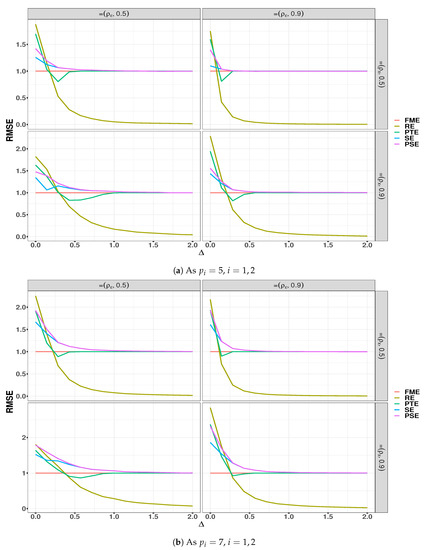
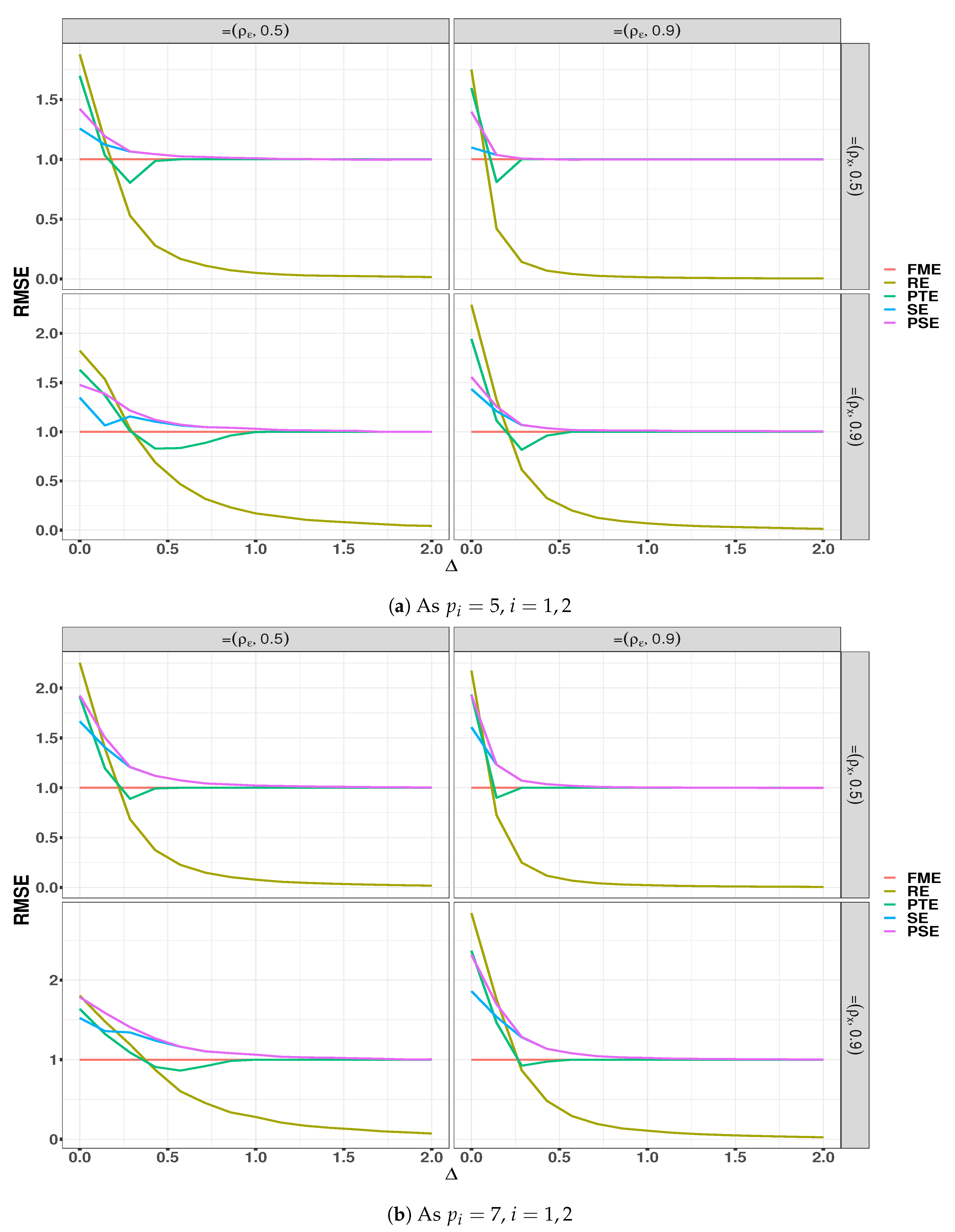
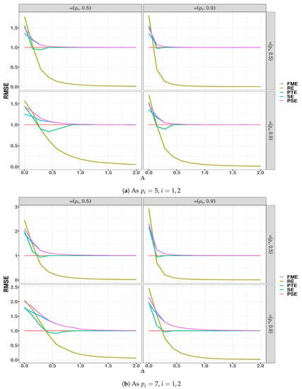
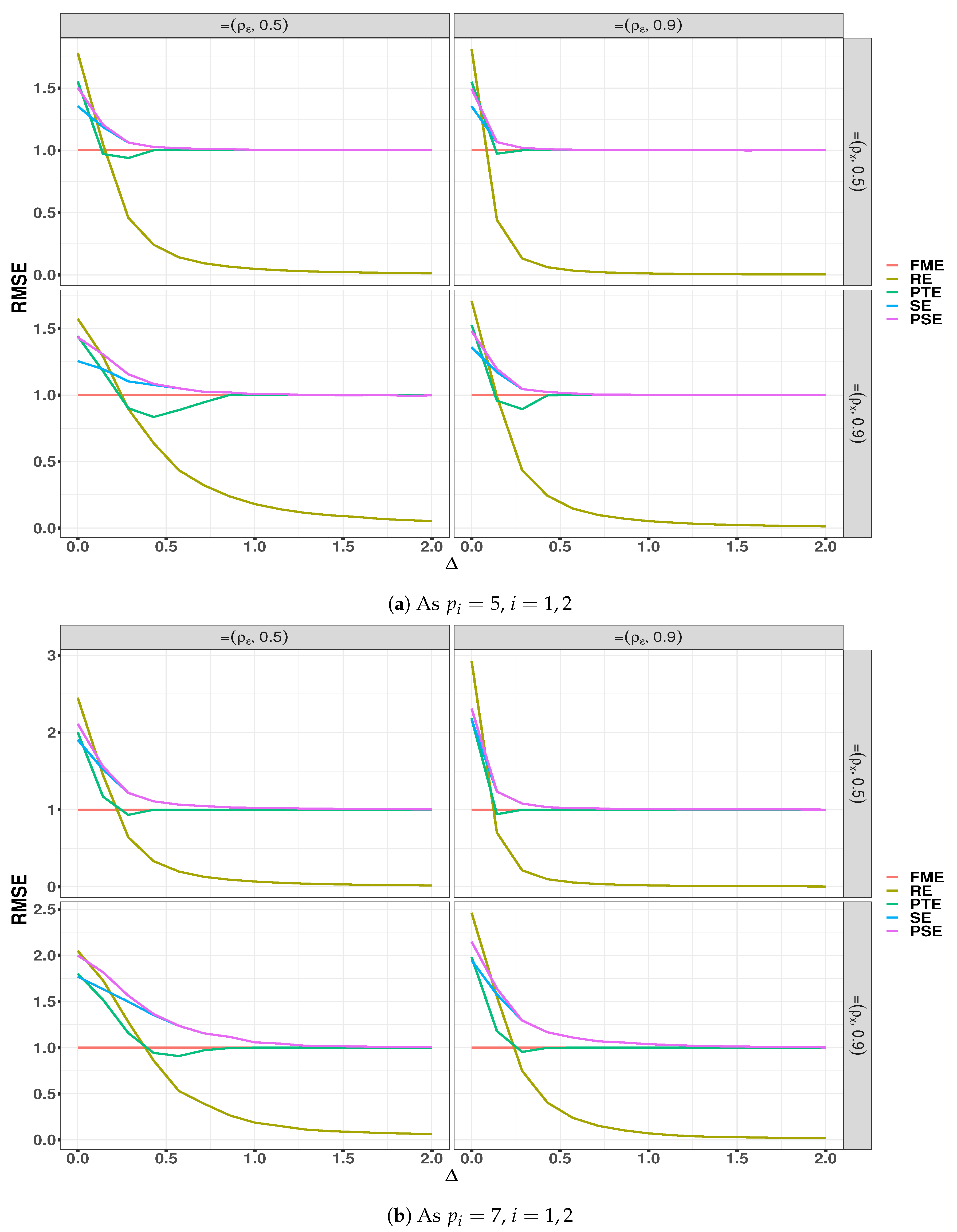
We plot the simulation results in Figure 1 and Figure 2. The simulation results for some other parameter configurations were also obtained, but are not included here for the sake of brevity.

Figure 1. RMSE of the estimators as a function of Δ when M = 2, T = 100, ρ_x = 0.5, 0.9, and ρ_ε = 0.5, 0.9. FME, full model estimator; RE, restricted estimation; PTE, preliminary test estimator; PSE, positive-rule Stein-type estimator.

Figure 2. RMSE of the estimators as a function of Δ when M = 3, T = 100, ρ_x = 0.5, 0.9, and ρ_ε = 0.5, 0.9.

According to these results:

1.

When $\mathsf{\Delta }=0$, which means that the null hypothesis is true or that the restrictions are consistent, the RE estimator always performs competitively when compared to other estimators. The PTE mostly outperforms the SE and PSE when $p_i=5$, while it looses its efficiency when $p_i=7$ when compared to PSE. The SE may perform worse than the FME due its sign problem, as is indicated in Section 3.

2.

When Δ > 0, which means that the null hypothesis is violated or the restrictions are invalid, the RE looses its efficiency, and its RMSE goes to zero, meaning that it becomes inconsistent. The RMSE of PTE decreases and remains below one for some values of Δ, but approaches one for larger values of Δ. The performance of PSE decreases, but its efficiency remains above the FME, for intermediate values of Δ, while it acts as the FME for larger values of Δ. It can be concluded that the PSE is a robust estimator even if the restriction is not true.

3.

We examined both medium and high correlation between disturbance terms. The results showed that the performance of suggested estimators was consistent with its theory; see Ahmed (2014).

4.

We examined both medium and high correlation between regressors across different equations. The results showed that the performance of suggested estimators was consistent with its theory; see Yüzbası et al. (2017).

5. Application

In the following section, we will apply the proposed estimation strategies to a financial dataset to examine the relative performance of the listed estimators. To illustrate and compare the listed estimators, we will study the effect of several economic and financial variables on the performance of the “Fragile Five” countries (coined by Stanley 2013) in terms of their attraction of direct foreign investment (FDI) over the period between 1983 and 2018. The “Fragile Five” include Turkey (TUR), South Africa (ZAF), Brazil (BRA), India (IND), and Indonesia (IDN). Agiomirgianakis et al. (2003), Hubert et al. (2017), and Akın (2019) used the FDI as the dependent variable across countries. With five countries, we have $M=5$ blocks in our SUR model, with measurements of $T=36$ years per equation. Table 2 provides information about prediction variables, and the raw data are available from the World Bank1.

Table 2. Descriptions of variables.

Variables	Descriptions
Dependent Variables
FDI	Foreign direct investment, net inflows (% of GDP)
Covariates
GROWTH	GDP per capita growth (annual %)
DEFLATOR	Inflation, GDP deflator (annual %)
EXPORTS	Exports of goods and services (% of GDP)
IMPORTS	Imports of goods and services (% of GDP)
GGFCE	General government final consumption expenditure (% of GDP)
RESERVES	Total reserves (includes gold, current US$)/GDP (current US$)
PREM	Personal remittances, received (% of GDP)
BALANCA	Current account balance (% of GDP)

We suggest the following model:

$$\begin{array}{ccc}\hfill {\mathrm{FDI}}_{it}& =\hfill & {\beta }_{0i}+{\beta }_{1i}\mathrm{GROWTH}+{\beta }_{2i}\mathrm{DEFLATOR}+{\beta }_{3i}\mathrm{EXPORTS}+{\beta }_{4i}\mathrm{IMPORTS}+\hfill \\ & & {\beta }_{5i}\mathrm{GGFCE}+{\beta }_{6i}\mathrm{RESERVES}+{\beta }_{7i}\mathrm{PREM}+{\beta }_{8i}\mathrm{BALANCE}+{ϵ}_{it},\hfill \end{array}$$

(14)

where i denotes countries $(i=\mathrm{TUR},\mathrm{ZAF},\mathrm{BRA},\mathrm{IND},\mathrm{IDN})$ and t is time $(t=1,2,\cdots ,T)$. Following Salman (2011), the errors of each equation are assumed to be normally distributed with mean zero, homoscedastic, and serially not autocorrelated. Furthermore, there is contemporaneous correlation between corresponding errors in different equations. We test these assumptions along with the assumptions in Section 2. We first check the following assumptions of each equation:

Nonautocorrelation of errors: There are a number of viable tests in the reviewed literature for testing the autocorrelation. For example, the Ljung–Box test is widely used in applications of time series analysis, and a similar assessment may be obtained via the Breusch–Godfrey test and the Durbin–Watson test. We apply the Ljung–Box test of (Ljung and Box 1978). The null hypothesis of the Ljung–Box Test, H₀, is that the errors are random and independent. A significant p-value in this test rejects the null hypothesis that the time series is not autocorrelated. Results reported in Table 3 suggest a rejection of H₀ for the equations of both TUR and IND at any conventional significance level. Thus, the estimation results will be clearly unsatisfactory for these two equation models. To tackle this problem, we performed the first differences procedure to transform the variables. After transformation, the test statistics and p-values of the equation TUR and IND were ${\chi }_{(1)}^2=1.379$, $p=0.240$ and ${\chi }_{(1)}^2=0.067$, $p=0.794$, respectively. Hence, each equation satisfied the assumption of nonautocorrelation. We confirmed our result using the Durbin–Watson test.

Table 3. Ljung-Box test.

Equation	Test Statistic	p-Value
TUR	${\chi }_{(1)}^2=6.853$	0.008
ZAF	${\chi }_{(1)}^2=0.704$	0.401
BRA	${\chi }_{(1)}^2=0.489$	0.483
IND	${\chi }_{(1)}^2=6.301$	0.012
IDN	${\chi }_{(1)}^2=1.061$	0.302

Homoscedasticity of errors: To test for heteroscedasticity, we used the Breusch–Pagan test (Breusch and Pagan 1979). The results in Table 4 failed to reject the null hypothesis in each equation.

Table 4. Breusch–Pagan test.

Equation	Test Statistic	p-Value
TUR	${\chi }_{(8)}^2=3.686$	0.884
ZAF	${\chi }_{(8)}^2=10.003$	0.264
BRA	${\chi }_{(8)}^2=7.544$	0.479
IND	${\chi }_{(8)}^2=6.455$	0.596
IDN	${\chi }_{(8)}^2=8.328$	0.402

The assumption homoscedasticity in each equation was thus met.

Normality of errors: To test for normality, there are various tests such as Shapiro–Wilk, Anderson–Darling, Cramer–von Mises, Kolmogorov–Smirnov, and Jarque–Bera. In this study, we performed the Jarque–Bera goodness-of-fit test (Jarque and Bera 1980).

The null hypothesis for the test is that the data are normally distributed. The results reported in Table 5 suggested a rejection of H₀ only for ZAF. We also performed the Kolmogorov–Smirnov test for ZAF, and the results showed that the errors were normally distributed. Thus, each equation satisfied the assumption of normality.

Table 5. Jarque–Bera test.

Equation	Test Statistic	p-Value
TUR	${\chi }_{(2)}^2=3.969$	0.137
ZAF	${\chi }_{(2)}^2=72.852$	0.000
BRA	${\chi }_{(2)}^2=2.355$	0.308
IND	${\chi }_{(2)}^2=1.815$	0.403
IDN	${\chi }_{(2)}^2=2.794$	0.247

Cross-sectional dependence: To test whether the estimated correlation between the sections was statistically significant, we applied the Breusch and Pagan (1980) Lagrange multiplier (LM) statistic and the Pesaran (2004) cross-section dependence (CD) tests. The null hypothesis of these tests claims there is no cross-section dependence. Both tests in Table 6 suggested a rejection of the null hypothesis that the residuals from each equation were significantly correlated with each other. Consequently, the SUR model would be the preferred technique, since this model assumed contemporaneous correlation across equations. Therefore, the joint estimation of all parameters rather than OLS, on each equation, was more efficient (Kleiber and Zeileis 2008).

Table 6. Cross-section dependence test results. LM, Lagrange multiplier; CD, cross-section dependence.

Correlation Matrix of Residuals
	TUR	ZAF	BRA	IND
ZAF	−0.207
BRA	0.066	−0.187
IND	0.414	−0.107	−0.016
IDN	0.128	−0.334	−0.064	0.235
Breusch and Pagan LM and Pesaran CD Tests
Test	Test Statistic		p-Value
LM	${\chi }_{(2)}^2=29.516$		0.001
CD	$Z=-4.353$		0.000

Specification test: The regression equation specification error test (RESET) designed by Ramsey (1969) is a general specification test for the linear regression model. It tests the exogeneity of the independent variables, that is the null hypothesis is $E\left[{\epsilon }_i|{\mathbf{X}}_i\right]=0$. Thus, rejecting the null hypothesis indicates that there is a correlation between the error term and the regressors or that nonlinearities exist in the functional form of the regression. The results reported in Table 7 suggested a rejection of H₀ only for IDN.

Table 7. The regression equation specification error test (RESET) test.

Equation	Test Statistic	p-Value
TUR	$F(8,18)=0.458$	0.869
ZAF	$F(8,19)=1.185$	0.357
BRA	$F(8,19)=1.062$	0.428
IND	$F(8,18)=1.648$	0.180
IDN	$F(8,19)=7.788$	0.000

Multicollinearity: We calculated the variance inflation factor (VIF) values among the predictors. A VIF value provides the user with a measure of how many times larger the Var$({\beta }_j)$ will be for multicollinear data than for orthogonal data. Usually, the multicollinearity is not a problem, as the VIFs are generally not significantly larger than one (Mansfield and Helms 1982). In the literature, values of VIF that exceed 10 are often regarded as indicating multicollinearity, but in weaker models, values above 2.5 may be a cause for concern. Another measure of multicollinearity is to calculate the condition number (CN) of ${\mathbf{X}}_i^{\prime }{\mathbf{X}}_i$, which is the square root of the ratio of the largest characteristic root of ${\mathbf{X}}_i^{\prime }{\mathbf{X}}_i$ to the smallest. Belsley et al. (2005) suggested that a CN greater than fifteen poses a concern, a CN in excess of 20 is indicative of a problem, and a CN close to 30 represents a severe problem. Table 8 displays the results from a series of multicollinearity diagnostics. In general, EXPORTS, IMPORTS, and BALANCE were found to be problematic with regard to VIF values, while the others may be a little concerning. On the other hand, the results from the CN test suggested that there was a very serious concern about multicollinearity for the equations of ZAF, BRA, and IDN. In light of these results, it was clear that the problem of multicollinearity existed in the equations. According to Greene (2019), the SUR estimation is more efficient when the less correlation exists between covariates. Therefore, the ridge-type SUR estimation will be a good solution of this problem.

Table 8. Variance inflation factor (VIF) and CN values.

Equation	GROWTH	DEFLATOR	EXPORTS	IMPORTS	GGFCE	RESERVES	PREM	BALANCE	CN
TUR	4.039	2.638	16.289	13.959	2.055	1.791	1.462	19.073	11.122
ZAF	3.070	7.354	69.891	191.248	3.891	12.918	5.847	60.728	248.221
BRA	1.204	1.614	18.324	32.159	6.329	3.131	3.938	13.301	85.336
IND	1.745	1.757	6.545	6.653	1.517	1.527	1.378	2.712	6.535
IDN	7.835	7.786	44.842	34.152	5.564	8.274	3.072	15.022	127.099

Structural change: To investigate the stability of the coefficients in each equation, we used the CUSUM (cumulative sum) test of Brown et al. (1975) that checks for structural changes. The null hypothesis is that of coefficient constancy, while the alternative suggests inconsistent structural change in the model over time. The results in Table 9 suggested the stability of coefficients over time.

Table 9. CUSUM test.

Equation	Test Statistic	p-Value
TUR	$T=0.734$	0.653
ZAF	$T=0.417$	0.995
BRA	$T=0.496$	0.966
IND	$T=0.413$	0.995
IDN	$T=0.401$	0.997

Following Lawal et al. (2019), we selected important variables in each equation of the SUR model and implemented the stepwise AIC forward regression by using the function ols_step_forward_aic from the olsrr package in the R project. The statistically significant variables are shown in Table 10. After that, the sub-models were constituted by using these variables per equation.

Table 10. Important variables per equation.

Equation	GROWTH	DEFLATOR	EXPORTS	IMPORTS	GGFCE	RESERVES	PREM	BALANCE
TUR			✓
ZAF							✓
BRA		✓		✓				✓
IND				✓			✓	✓
IDN			✓	✓			✓

In light of the selected variables in Table 10, we construct the matrices of restrictions as follows:

$$\begin{array}{ccc}\hfill {\mathbf{R}}_1& =& \left[\begin{array}{cccccccc}1& 0& 0& 0& 0& 0& 0& 0\\ 0& 1& 0& 0& 0& 0& 0& 0\\ 0& 0& 0& 1& 0& 0& 0& 0\\ 0& 0& 0& 0& 1& 0& 0& 0\\ 0& 0& 0& 0& 0& 1& 0& 0\\ 0& 0& 0& 0& 0& 0& 1& 0\\ 0& 0& 0& 0& 0& 0& 0& 1\end{array}\right],{\mathbf{R}}_2=\left[\begin{array}{cccccccc}1& 0& 0& 0& 0& 0& 0& 0\\ 0& 1& 0& 0& 0& 0& 0& 0\\ 0& 0& 1& 0& 0& 0& 0& 0\\ 0& 0& 0& 1& 0& 0& 0& 0\\ 0& 0& 0& 0& 1& 0& 0& 0\\ 0& 0& 0& 0& 0& 1& 0& 0\\ 0& 0& 0& 0& 0& 0& 0& 1\end{array}\right],{\mathbf{r}}_1={\mathbf{r}}_2=\left[\begin{array}{c}0\\ 0\\ 0\\ 0\\ 0\\ 0\\ 0\end{array}\right],\hfill \\ \hfill {\mathbf{R}}_3& =& \left[\begin{array}{cccccccc}1& 0& 0& 0& 0& 0& 0& 0\\ 0& 0& 1& 0& 0& 0& 0& 0\\ 0& 0& 0& 0& 1& 0& 0& 0\\ 0& 0& 0& 0& 0& 1& 0& 0\\ 0& 0& 0& 0& 0& 0& 1& 0\end{array}\right],{\mathbf{R}}_4=\left[\begin{array}{cccccccc}0& 1& 0& 0& 0& 0& 0& 0\\ 0& 0& 1& 0& 0& 0& 0& 0\\ 0& 0& 0& 0& 1& 0& 0& 0\\ 0& 0& 0& 0& 0& 0& 1& 0\\ 0& 0& 0& 0& 0& 0& 0& 1\end{array}\right],\hfill \\ \hfill {\mathbf{R}}_5& =& \left[\begin{array}{cccccccc}1& 0& 0& 0& 0& 0& 0& 0\\ 0& 1& 0& 0& 0& 0& 0& 0\\ 0& 0& 0& 0& 1& 0& 0& 0\\ 0& 0& 0& 0& 0& 1& 0& 0\\ 0& 0& 0& 0& 0& 0& 0& 1\end{array}\right]\mathrm{and}{\mathbf{r}}_3={\mathbf{r}}_4={\mathbf{r}}_5=\left[\begin{array}{c}0\\ 0\\ 0\\ 0\\ 0\end{array}\right];\hfill \end{array}$$

thus, the reduced models are given by:

$$\begin{array}{ccc}\hfill \mathrm{TUR}& :& {\mathrm{FDI}}_t={\beta }_0+{\beta }_3\mathrm{EXPORTS}+{ϵ}_t,\hfill \end{array}$$

(15)

$$\begin{array}{ccc}\hfill \mathrm{ZAF}& :& {\mathrm{FDI}}_t={\beta }_0+{\beta }_7\mathrm{PREM}+{ϵ}_t,\hfill \end{array}$$

(16)

$$\begin{array}{ccc}\hfill \mathrm{BRA}& :& {\mathrm{FDI}}_t={\beta }_0+{\beta }_2\mathrm{DEFLATOR}+{\beta }_4\mathrm{IMPORTS}+{\beta }_8\mathrm{BALANCE}+{ϵ}_t,\hfill \end{array}$$

(17)

$$\begin{array}{ccc}\hfill \mathrm{IND}& :& {\mathrm{FDI}}_t={\beta }_0+{\beta }_4\mathrm{IMPORTS}+{\beta }_7\mathrm{PREM}+{\beta }_8\mathrm{BALANCE}+{ϵ}_t,\hfill \end{array}$$

(18)

$$\begin{array}{ccc}\hfill \mathrm{IDN}& :& {\mathrm{FDI}}_t={\beta }_0+{\beta }_3\mathrm{EXPORTS}+{\beta }_4\mathrm{IMPORTS}+{\beta }_7\mathrm{PREM}+{ϵ}_t,\hfill \end{array}$$

(19)

Next, we combined Model (14) and Models (15)–(19) using the shrinkage and preliminarily test strategies outlined in Section 3. Before we performed our analysis, the response was centred, and the predictors were standardized for each equation so that the intercept term was omitted. We then split the data by using the time series cross-validation technique of Hyndman and Athanasopoulos (2018) into a series of training sets and a series of testing sets. Each test set consisted of a single observation for the models that produced one step-ahead forecasts. In this procedure, the observations in the corresponding training sets occurred prior to the observation of the test sets. Hence, it was ensured that no future observations could be used in constructing the forecast. We used the function createTimeSlices from the caret package in the R project here. The listed models were applied to the data, and predictions were made based on the divided training and test sets. The process was repeated 15 times, and for each subset’s prediction, the mean squared error (MSE) and the mean absolute error (MAE) were calculated. The means of the 15 MSEs and MAEs were then used to evaluate the performance for each method. We also report the relative performances (RMAE and RMSE) with respect to the full model estimator for easier comparison. If a relative value of an estimator is larger than one, it is superior to the full model estimator.

In Table 11, we report the MSE and MAE values and their standard errors to see the stability of the algorithm. Based on this table, as expected, the RE had the smallest measurement values since the insignificant variables were selected as close to correct as possible. We saw that the performance of the PSE after the RE was best by following the SE and the PTE. Moreover, the performance of the OLS was the worst due to the problem of multicollinearity.

Table 11. Comparison of forecasting performance.

	RE	FME	PTE	SE	PSE	OLS
MAE	0.572 (0.114)	1.076 (0.148)	0.656 (0.139)	0.649 (0.124)	0.646 (0.122)	1.166 (0.165)
RMAE	1.879	1	1.639	1.656	1.664	0.922
MSE	0.598 (0.061)	0.800 (0.062)	0.624 (0.067)	0.624 (0.069)	0.622 (0.068)	0.831 (0.064)
RMSE	1.338	1	1.283	1.282	1.287	0.963

The numbers in parenthesis are the corresponding standard errors of the MAE and MSE.

In order to test whether the two competing models had the same forecasting accuracy, we used the two-sided statistical Diebold–Mariano (DM) test (Diebold and Mariano 1995) when the forecasting horizon was extended to one year, and the loss functions were both squared errors and absolute errors. A significant p-value in this test rejected the null hypothesis that the models had different forecasting accuracy. The results based on the absolute-error loss in Table 12 suggested that the FME had different prediction accuracy with all methods except RE. Additionally, the forecasting accuracy of the OLS differed from the listed estimators. On the other hand, the results of the DM test based on the squared error loss suggested that the observed differences between the RE and shrinkage estimators were significant.

Table 12. Diebold–Mariano test for the forecasting results.

LF		FME	RE	PTE	SE	PSE
MAE	RE	−1.308 (0.191)
	PTE	−2.601 (0.009 ***)	−0.608 (0.543)
	SE	−2.146 (0.032 **)	−0.733 (0.463)	0.276 (0.783)
	PSE	−2.163 (0.031 **)	−0.702 (0.483)	0.33 (0.741)	0.551 (0.582)
	OLS	3.734 (0.000 ***)	1.700 (0.089 *)	2.972 (0.003 ***)	2.543 (0.011 **)	2.56 (0.010 **)
MSE	SM	−0.187 (0.852)
	PTE	−1.968 (0.049 **)	−2.165 (0.030 **)
	SE	−1.444 (0.149)	−2.392 (0.017 **)	1.443 (0.149)
	PSE	−1.474 (0.140)	−2.374 (0.018 **)	1.436 (0.151)	−1.496 (0.135)
	OLS	3.528 (0.000 ***)	0.691 (0.490)	2.379 (0.017 **)	1.904 (0.057 *)	1.933 (0.053 *)

The numbers in parenthesis are the corresponding p-values; LS is the “loss function” of the method to compute; * p < 0.1, ** p < 0.05, *** p < 0.01.

Finally, the estimates of coefficients of all countries are given in Table 13.

Table 13. Estimated coefficients.

Estimation	Country	GROWTH	DEFLATOR	EXPORTS	IMPORTS	GGFCE	RESERVES	PREM	BALANCE
RE	TUR	0 (0)	0 (0)	0.102 (0.003)	0 (0)	0 (0)	0 (0)	0 (0)	0 (0)
	ZAF	0 (0)	0 (0)	0 (0)	0 (0)	0 (0)	0 (0)	0.509 (0.007)	0 (0)
	BRA	0 (0)	−0.231 (0.005)	0 (0)	0.912 (0.005)	0 (0)	0 (0)	0 (0)	−0.377 (0.006)
	IND	−0.113 (0.002)	0 (0)	0 (0)	0.122 (0.003)	0 (0)	0.052 (0.002)	0 (0)	0 (0)
	IDN	0 (0)	0 (0)	−1.903 (0.015)	1.341 (0.014)	0 (0)	0 (0)	0.427 (0.004)	0 (0)
FME	TUR	−0.369 (0)	−0.064 (0)	0.327 (0.003)	−0.187 (0)	−0.140 (0)	0.036 (0)	0.061 (0)	−0.543 (0)
	ZAF	−0.120 (0)	−0.397 (0)	0.521 (0)	−0.139 (0)	0.012 (0)	−0.810 (0)	0.551 (0.007)	−0.420 (0)
	BRA	0.059 (0)	−0.18 (0.005)	0.999 (0)	−0.265 (0.005)	0.859 (0)	0.004 (0)	−0.210 (0)	−1.042 (0.006)
	IND	−0.071 (0.002)	0.018 (0)	−0.091 (0)	0.253 (0.003)	−0.002 (0)	−0.024 (0.002)	0.149 (0)	0.150 (0)
	IDN	0.280 (0)	0.177 (0)	−2.348 (0.015)	1.689 (0.014)	−0.009 (0)	−0.233 (0)	0.475 (0.004)	0.242 (0)
PTE	TUR	−0.151 (0)	−0.026 (0)	0.188 (0.003)	−0.072 (0)	−0.058 (0)	0.014 (0)	0.026 (0)	−0.219 (0)
	ZAF	−0.048 (0)	−0.140 (0)	0.184 (0)	−0.014 (0)	0.012 (0)	−0.318 (0)	0.514 (0.007)	−0.160 (0)
	BRA	0.024 (0)	−0.215 (0.005)	0.420 (0)	0.404 (0.005)	0.350 (0)	0.011 (0)	−0.073 (0)	−0.664 (0.006)
	IND	−0.094 (0.002)	0.006 (0)	−0.032 (0)	0.174 (0.003)	0.003 (0)	0.021 (0.002)	0.059 (0)	0.062 (0)
	IDN	0.126 (0)	0.064 (0)	−2.072 (0.015)	1.475 (0.014)	−0.002 (0)	−0.087 (0)	0.445 (0.004)	0.094 (0)
SE	TUR	−0.110 (0)	−0.019 (0)	0.166 (0.003)	−0.053 (0)	−0.042 (0)	0.010 (0)	0.018 (0)	−0.160 (0)
	ZAF	−0.036 (0)	−0.108 (0)	0.142 (0)	−0.022 (0)	0.006 (0)	−0.237 (0)	0.517 (0.007)	−0.119 (0)
	BRA	0.017 (0)	−0.218 (0.005)	0.299 (0)	0.554 (0.005)	0.253 (0)	0.005 (0)	−0.057 (0)	−0.579 (0.006)
	IND	−0.100 (0.002)	0.005 (0)	−0.025 (0)	0.160 (0.003)	0.001 (0)	0.029 (0.002)	0.043 (0)	0.045 (0)
	IDN	0.088 (0)	0.048 (0)	−2.031 (0.015)	1.442 (0.014)	−0.002 (0)	−0.065 (0)	0.440 (0.004)	0.070 (0)
PSE	TUR	−0.112 (0)	−0.019 (0)	0.168 (0.003)	−0.055 (0)	−0.043 (0)	0.010 (0)	0.019 (0)	−0.164 (0)
	ZAF	−0.037 (0)	−0.112 (0)	0.146 (0)	−0.023 (0)	0.006 (0)	−0.243 (0)	0.517 (0.007)	−0.122 (0)
	BRA	0.018 (0)	−0.217 (0.005)	0.307 (0)	0.546 (0.005)	0.260 (0)	0.005 (0)	−0.059 (0)	−0.584 (0.006)
	IND	−0.099 (0.002)	0.005 (0)	−0.026 (0)	0.161 (0.003)	0.001 (0)	0.029 (0.002)	0.044 (0)	0.046 (0)
	IDN	0.090 (0)	0.050 (0)	−2.033 (0.015)	1.444 (0.014)	−0.002 (0)	−0.067 (0)	0.441 (0.004)	0.071 (0)
OLS	TUR	−0.400 (0)	−0.071 (0)	0.379 (0.003)	−0.230 (0)	−0.147 (0)	0.042 (0)	0.066 (0)	−0.618 (0)
	ZAF	−0.142 (0)	−0.443 (0)	0.648 (0)	−0.291 (0)	0.007 (0)	−0.916 (0)	0.613 (0.007)	−0.515 (0)
	BRA	0.067 (0)	−0.171 (0.005)	1.078 (0)	−0.327 (0.005)	0.909 (0)	−0.018 (0)	−0.225 (0)	−1.110 (0.006)
	IND	−0.074 (0.002)	0.020 (0)	−0.105 (0)	0.275 (0.003)	−0.004 (0)	−0.029 (0.002)	0.156 (0)	0.163 (0)
	IDN	0.270 (0)	0.179 (0)	−2.468 (0.015)	1.768 (0.014)	−0.016 (0)	−0.246 (0)	0.478 (0.004)	0.281 (0)

The numbers in parenthesis are the corresponding standard errors.

6. Conclusions

In this paper, we proposed the shrinkage and preliminary test estimation methods in a system of regression models when the disturbances were dependent and correlations existed among regressors in each equation. To build the model, we first multiplied both sides of Model (1) by the inverse variance–covariance matrix of the disturbances and transformed the values using spectral decomposition. We defined the full model estimator by following Alkhamisi and Shukur (2008) and the restricted estimator by assuming a UNPI on the vector of parameters. Finally, we combined them in an optimal way by applying the shrinkage and preliminary test strategies. To illustrate and compare the relative performance of these methods, we conducted a Monte Carlo simulation. The simulated results demonstrated that the RE outperformed all other estimators when there was sufficient evidence that the vector nuisance parameters were a zero vector, that is Δ = 0. However, the RE lost its efficiency as Δ increased and became unbounded when Δ was large. The PSE dominated the FME at the small values of Δ, while the SE and PSE outshone the FME in the entire parametric space. However, the PSE was better than the SE because it controlled for the over-shrinking problem in SE. We also investigated the performance of the suggested estimations via a real-world example using financial data for the “Fragile Five” countries. The results of our data analysis were consistent with the simulated results.

For further research, one can use the other penalized techniques for the SUR model such as the smoothly clipped absolute deviation (SCAD) by Fan and Li (2001), the least absolute shrinkage and selection operator (LASSO) by Tibshirani (1996), and the adaptive LASSO estimators by Zou (2006), as well as our preliminary and shrinkage estimations.

References

- Agiomirgianakis, George Myron, Dimitrios Asteriou, and Kalliroi Papathoma. 2003. The Determinants of Foreign Direct Investment: A Panel Data Study for the Oecd Countries. Monograph (Discussion Paper). London: Department of Economics, City University London. [Google Scholar]
- Ahmed, S. Ejaz. 2014. Penalty, Shrinkage and Pretest Strategies: Variable Selection and Estimation. New York: Springer. [Google Scholar]
- Ahmed, S. Ejaz, and Bahadır Yüzbaşı. 2016. Big data analytics: Integrating penalty strategies. International Journal of Management Science and Engineering Management 11: 105–15. [Google Scholar] [CrossRef] [Scilit]
- Akın, Tuğba. 2019. The effects of political stability on foreign direct investment in fragile five countries. Central European Journal of Economic Modelling and Econometrics 11: 237–55. [Google Scholar]
- Alkhamisi, M. A. 2010. Simulation study of new estimators combining the sur ridge regression and the restricted least squares methodologies. Statistical Papers 51: 651–72. [Google Scholar] [CrossRef] [Scilit]
- Alkhamisi, M. A., and Ghazi Shukur. 2008. Developing ridge parameters for sur model. Communications in Statistics—Theory and Methods 37: 544–64. [Google Scholar] [CrossRef] [Scilit]
- Arashi, Mohammad, and Mahdi Roozbeh. 2015. Shrinkage estimation in system regression model. Computational Statistics 30: 359–76. [Google Scholar] [CrossRef] [Scilit]
- Barari, Mahua, and Srikanta Kundu. 2019. The role of the federal reserve in the us housing crisis: A var analysis with endogenous structural breaks. Journal of Risk and Financial Management 12: 125. [Google Scholar] [CrossRef] [Scilit]
- Belsley, David A., Edwin Kuh, and Roy E. Welsch. 2005. Regression Diagnostics: Identifying Influential Data and Sources of Collinearity. Hoboken: John Wiley & Sons, vol. 571. [Google Scholar]
- Breusch, Trevor S., and Adrian R. Pagan. 1979. A simple test for heteroscedasticity and random coefficient variation. Econometrica: Journal of the Econometric Society 47: 1287–94. [Google Scholar] [CrossRef] [Scilit]
- Breusch, Trevor S., and Adrian R. Pagan. 1980. The lagrange multiplier test and its applications to model specification in econometrics. The Review of Economic Studies 47: 239–53. [Google Scholar] [CrossRef] [Scilit]
- Brown, Robert L., James Durbin, and James M. Evans. 1975. Techniques for testing the constancy of regression relationships over time. Journal of the Royal Statistical Society: Series B (Methodological) 37: 149–63. [Google Scholar] [CrossRef] [Scilit]
- Diebold, Francis X., and Robert S. Mariano. 1995. Comparing predictive accuracy. Journal of Business & Economic Statistics 20: 134–44. [Google Scholar]
- Dincer, Oguzhan C., and Fan Wang. 2011. Ethnic diversity and economic growth in China. Journal of Economic Policy Reform 14: 1–10. [Google Scholar] [CrossRef] [Scilit]
- Erdugan, Funda, and Fikri Akdeniz. 2016. Restricted estimator in two seemingly unrelated regression model. Pakistan Journal of Statistics and Operation Research 12: 579–88. [Google Scholar] [CrossRef] [Scilit]
- Fan, Jianqing, and Runze Li. 2001. Variable selection via nonconcave penalized likelihood and its oracle properties. Journal of the American Statistical Association 96: 1348–60. [Google Scholar] [CrossRef] [Scilit]
- Gao, Xiaoli, S. E. Ahmed, and Yang Feng. 2017. Post selection shrinkage estimation for high-dimensional data analysis. Applied Stochastic Models in Business and Industry 33: 97–120. [Google Scholar] [CrossRef] [Scilit]
- Greene, William H. 2019. Econometric Analysis. Harlow: Pearson. [Google Scholar]
- Groß, Jürgen. 2003. Restricted ridge estimation. Statistics & Probability Letters 65: 57–64. [Google Scholar]
- Henningsen, Arne, and Jeff D. Hamann. 2007. Systemfit: A package for estimating systems of simultaneous equations in r. Journal of Statistical Software 23: 1–40. [Google Scholar] [CrossRef] [Scilit]
- Hoerl, Arthur E., and Robert W. Kennard. 1970. Ridge regression: Biased estimation for nonorthogonal problems. Technometrics 12: 55–67. [Google Scholar] [CrossRef]
- Hubert, Mia, Tim Verdonck, and Özlem Yorulmaz. 2017. Fast robust sur with economical and actuarial applications. Statistical Analysis and Data Mining: The ASA Data Science Journal 10: 77–88. [Google Scholar] [CrossRef] [Scilit]
- Hyndman, Rob J., and George Athanasopoulos. 2018. Forecasting: Principles and Practice. Melbourne: OTexts. [Google Scholar]
- James, W., and C. Stein. 1961. Proc. fourth berkeley symp. math. statist. probab. In Estimation with Quadratic Loss. Berkeley: University California Press, vol. 1, pp. 361–79. [Google Scholar]
- Jarque, Carlos M., and Anil K. Bera. 1980. Efficient tests for normality, homoscedasticity and serial independence of regression residuals. Economics Letters 6: 255–59. [Google Scholar] [CrossRef] [Scilit]
- Kaçıranlar, Selahattin, Sadullah Sakallıoğlu, M. Revan Özkale, and Hüseyin Güler. 2011. More on the restricted ridge regression estimation. Journal of Statistical Computation and Simulation 81: 1433–48. [Google Scholar] [CrossRef] [Scilit]
- Kleiber, Christian, and Achim Zeileis. 2008. Applied Econometrics with R. Heidelberg: Springer Science & Business Media. [Google Scholar]
- Kuan, C.-M. 2004. Introduction to Econometric Theory. Lecture Notes. Available online: ftp://nozdr.ru/biblio/kolxoz/G/GL/Kuan%20C.-M.%20Introduction%20to%20econometric%20theory%20(LN,%20Taipei,%202002)(202s)_GL_.pdf (accessed on 18 June 2020).
- Lawal, Afeez Abolaji, and Oluwayemesi Oyeronke Alaba. 2019. Exploratory analysis of some sectors of the economy: A seemingly unrelated regression approach. African Journal of Applied Statistics 6: 649–61. [Google Scholar] [CrossRef] [Scilit]
- Ljung, Greta M., and George E. P. Box. 1978. On a measure of lack of fit in time series models. Biometrika 65: 297–303. [Google Scholar] [CrossRef]
- Mansfield, Edward R., and Billy P. Helms. 1982. Detecting multicollinearity. The American Statistician 36: 158–60. [Google Scholar]
- Pesaran, M. Hashem. 2004. General Diagnostic Tests for Cross Section Dependence in Panels. CESifo Working Papers. Cambridge: University of Cambridge, Faculty of Economics. [Google Scholar]
- Ramsey, James Bernard. 1969. Tests for specification errors in classical linear least-squares regression analysis. Journal of the Royal Statistical Society: Series B (Methodological) 31: 350–71. [Google Scholar] [CrossRef] [Scilit]
- Salman, A. Khalik. 2011. Using the sur model of tourism demand for neighbouring regions in sweden and norway. In Advances in Econometrics-Theory and Applications. London: IntechOpen. 98p. [Google Scholar]
- Shukur, Ghazi. 2002. Dynamic specification and misspecification in systems of demand equations: A testing strategy for model selection. Applied Economics 34: 709–25. [Google Scholar] [CrossRef] [Scilit]
- Srivastava, Virendera K., and David E. A. Giles. 1987. Seemingly Unrelated Regression Equations Models: Estimation and Inference. New York: CRC Press, vol. 80. [Google Scholar]
- Srivastava, Viren K., and Alan T. K. Wan. 2002. Separate versus system methods of stein-rule estimation in seemingly unrelated regression models. Communications in Statistics—Theory and Methods 31: 2077–99. [Google Scholar] [CrossRef] [Scilit]
- Stanley, Morgan. 2013. Fx pulse preparing for volatility. Global Outlook 1: 1–37. [Google Scholar]
- Tibshirani, Robert. 1996. Regression shrinkage and selection via the lasso. Journal of the Royal Statistical Society: Series B (Methodological) 58: 267–88. [Google Scholar] [CrossRef] [Scilit]
- Williams, Barry. 2013. Income volatility of indonesian banks after the asian financial crisis. Journal of the Asia Pacific Economy 18: 333–58. [Google Scholar] [CrossRef] [Scilit]
- Yüzbası, Bahadır, S. Ejaz Ahmed, and Mehmet Güngör. 2017. Improved penalty strategies in linear regression models. REVSTAT–Statistical Journal 15: 251–76. [Google Scholar]
- Yüzbaşı, Bahadır, Mohammad Arashi, and S. Ejaz Ahmed. 2020. Shrinkage estimation strategies in generalised ridge regression models: Low/high-dimension regime. International Statistical Review 88: 229–51. [Google Scholar] [CrossRef] [Scilit]
- Zeebari, Zangin, B. M. Golam Kibria, and Ghazi Shukur. 2018. Seemingly unrelated regressions with covariance matrix of cross-equation ridge regression residuals. Communications in Statistics-Theory and Methods 47: 5029–53. [Google Scholar] [CrossRef] [Scilit]
- Zeebari, Zangin, Ghazi Shukur, and B. M. G. Kibria. 2012. Modified ridge parameters for seemingly unrelated regression model. Communications in Statistics-Theory and Methods 41: 1675–91. [Google Scholar] [CrossRef] [Scilit]
- Zellner, Arnold. 1962. An efficient method of estimating seemingly unrelated regressions and tests for aggregation bias. Journal of the American statistical Association 57: 348–68. [Google Scholar] [CrossRef]
- Zou, Hui. 2006. The adaptive lasso and its oracle properties. Journal of the American Statistical Association 101: 1418–29. [Google Scholar] [CrossRef] [Scilit]