The Predictability of the Exchange Rate When Combining Machine Learning and Fundamental Models

Abstract

In 1983, Meese and Rogoff showed that traditional economic models developed since the 1970s do not perform better than the random walk in predicting out-of-sample exchange rates when using data obtained after the beginning of the floating rate system. Subsequently, whether traditional economical models can ever outperform the random walk in forecasting out-of-sample exchange rates has received scholarly attention. Recently, a combination of fundamental models with machine learning methodologies was found to outcompete the predictability of random walk (Amat et al. 2018). This paper focuses on combining modern machine learning methodologies with traditional economic models and examines whether such combinations can outperform the prediction performance of random walk without drift. More specifically, this paper applies the random forest, support vector machine, and neural network models to four fundamental theories (uncovered interest rate parity, purchase power parity, the monetary model, and the Taylor rule models). We performed a thorough robustness check using six government bonds with different maturities and four price indexes, which demonstrated the superior performance of fundamental models combined with modern machine learning in predicting future exchange rates in comparison with the results of random walk. These results were examined using a root mean squared error (RMSE) and a Diebold–Mariano (DM) test. The main findings are as follows. First, when comparing the performance of fundamental models combined with machine learning with the performance of random walk, the RMSE results show that the fundamental models with machine learning outperform the random walk. In the DM test, the results are mixed as most of the results show significantly different predictive accuracies compared with the random walk. Second, when comparing the performance of fundamental models combined with machine learning, the models using the producer price index (PPI) consistently show good predictability. Meanwhile, the consumer price index (CPI) appears to be comparatively poor in predicting exchange rate, based on its poor results in the RMSE test and the DM test.

1. Introduction

Despite the existence of various economic theories explaining the fluctuation of future exchange rates, as shown in Meese and Rogoff (1983a, 1983b), the random walk often produces better predictions for future exchange rates. More specifically, it has been shown that traditional economical models developed since the 1970s do not perform better than the random walk in predicting the out-of-sample exchange rate when using data obtained after the beginning of the floating rate system. Since the publication of these papers, many researchers have investigated this puzzle. Cheung et al. (2005) confirmed the work of Meese and Rogoff (1983a, 1983b), and demonstrated that the interest rate parity, monetary, productivity-based, and behavioral exchange rate models do not outperform the random walk for any time-period. Similarly, Rossi (2013) could not find a model with strong out-of-sample forecasting ability. On the contrary, Mark (1995) showed that the economic exchange-rate models perform better than the random walk in predicting long term exchange rates. Amat et al. (2018) also found that combining machine learning methodologies, traditional exchange-rate models, and Taylor-rule exchange rate models could be useful in forecasting future short-term exchange rates in the case of 12 major currencies.

There have been similar attempts by researchers using stock market data. These studies show the predictability of future stock price using machine learning methodologies (Cervelló-Royo et al. 2015; Chong et al. 2017), and stock market trends (Chang et al. 2012; García et al. 2018). Hamori et al. (2018) also analyzed the default risk using several machine learning techniques.

Following on from these previous studies, this paper focuses on a combination of modern machine learning methodologies and economic models. The purpose of this paper is to determine whether such combinations outperform the prediction performance of random walk without drift. This model has been used as the comparison in most studies in this field since Meese and Rogoff (1983a, 1983b). The most profound study in this field is Amat et al. (2018). What distinguishes the present paper from previous studies is that instead of using an exponential weighted average strategy and sequential ridge regression with discount factors, this paper applies the random forest, support vector machine (SVM), and neural network models to four fundamental theories (uncovered interest rate parity, purchase power parity, the monetary model, and the Taylor rule models). Furthermore, the robustness of the results is thoroughly examined using six government bonds with different maturities (1, 2, 3, 5, 7, and 10 years) and four price indexes (the producer price index (PPI), the consumer price index (CPI) of all items, CPI excluding fresh food, and CPI excluding fresh food and energy) individually in three machine learning models. Together, these elements should provide concrete evidence for the results that were obtained.

In the empirical analysis, a rolling window analysis was used for a one-period-ahead forecast for the JPY/USD exchange rate. The sample data range from August 1980 until August 2019. The window size was set as 421. Hence, in total, the rolling window analysis was conducted 47 times for the individual fundamental models. The main findings of this study are as follows. First, when comparing the performance of the fundamental models combined with machine learning to that of the random walk, the root mean squared error (RMSE) results show that the fundamental models with machine learning outperform the random walk (the mean absolute percentage error (MAPE) also confirmed this result). In the Diebold–Mariano (DM) test, most of the results show significantly different predictive accuracies compared to the random walk, while some of the random forest results show the same accuracy as the random walk. Second, when comparing the performance of the fundamental models combined with machine learning, the models using the PPI show fairly good predictability in a consistent manner. This is indicated by both the RMSE and the DM test results. However, the CPI is not appropriate for predicting exchange rates, based on its poor results in the RMSE test and DM test. This result seems reasonable given that the CPI includes volatile price indicators such as food, beverages and energy.

The rest of the paper is organized as follows. Section 2 explains the fundamental models, Section 3 describes the data used in the empirical studies, Section 4 describes the methodology of machine learning, Section 5 shows the results and evaluation, and Section 6 summarizes the main findings of the paper.

2. Fundamental Models

Following Rossi (2013) and Amat et al. (2018), this paper uses four basic methods to predict the exchange rate. These methods are uncovered interest rate parity (UIRP), purchase power parity (PPP), the monetary model, and the Taylor rule models.

2.1. Uncovered Interest Rate Parity

The UIRP theorem used in the following section was proposed by Fisher (1896). This theorem analyzes how interest rates can be altered due to expected changes in the relative value of the objected units. UIRP is based on the following assumption; in a world with only two currencies and where market participants possess perfect information, investors can buy $1=S_t$ units of foreign government bonds using one unit of their home currency. When investors buy a foreign bond between time $t$ and time $t+h$, the earnings from the foreign bond are the bond premium plus the foreign interest rate: $i_{t+h}^{*}$. At the end of the period, investors can collect the return converted to the home currency, which is shown as $S_{t+h}\left[\left(1+i_{t+h}^{*}\right)/S_t\right]$ in expectation. Additional transaction costs during the whole process are ignored in this analysis, and the bond return should be the same whether the investors buy the home bond or the foreign bond. Hence, the following equation is given:

$$\left(1+i_{t+h}^{*}\right)E_t(S_{t+h}/S_t)=1+i_{t+h}$$

(1)

By taking logarithms, the previous UIRP equation can be rewritten as

$$E_t\left(s_{t+h}-s_t\right)=\alpha +\beta \left(i_{t+h}-i_{t+h}^{*}\right)$$

(2)

where $S_t$ is the logarithm of the exchange rate, and $h$ is the horizon.

Another uncovered interest rate parity equation used in Taylor (1995) is as follows:

$${\mathsf{\Delta }}_k{s}_{t+k}^e=i_t-i_t^{*}$$

(3)

where $s_t$ denotes the logarithm of the spot exchange rate (domestic price for foreign currency) at time $t$, and $i_t$ is the nominal interest for domestic and foreign securities, respectively (with $k$ periods to maturity).

It is worth noting that in both equations, maturity is denoted as $k$, meaning that if we follow the equation faithfully to predict the one-month ahead exchange rate, we should use the one-month maturity of the government bond to predict that rate. However, the focus here is on the relationship between interest rate differences and the exchange rate. Thus, the above equations are rewritten as

$$s_{t+1}-s_t=i_t-i_t^{*}.$$

(4)

The above equation is used in the following empirical analysis.

Meese and Rogoff (1983a, 1983b), who used Equation (1) to forecast sample real exchange rates using the real interest rates and compared their performance with the predictions using random walk, found that the latter provided better forecasting results.

2.2. Purchasing Power Parity

The PPP was first proposed in Cassel (1918). The concept of PPP is that the same amount of goods or services can be purchased in either currency with the same initial amount of currency. That is, a unit of currency in the home country would have the same purchasing power in the foreign country.

The absolute purchase power parity can be expressed as the following equation:

$$S=\frac{P}{P^{*}}$$

(5)

where $S$ denotes the exchange rate in period $t$, $P$ denotes the price level in the home country, and $P^{*}$ denotes the price level in the foreign country.

Assuming that the absolute purchasing power parity holds in period $t+1$, we can obtain the following equation:

$$S_{t+1}=\frac{P_{t+1}}{P_{t+1}^{*}}.$$

(6)

Assuming that the inflation rate from period $t$ to period $t+1$ is $\pi$, we can obtain following equation:

$$S_{t+1}=\frac{\left(1+\pi \right)P_t}{\left(1+{\pi }^{*}\right)P_t^{*}}=\frac{1+\pi }{1+{\pi }^{*}}{S}_t,$$

(7)

which means that

$$\frac{S_{t+1}}{S_t}=\frac{1+\pi }{1+{\pi }^{*}}.$$

(8)

Assuming that the rate of the change in the exchange rate is $\rho$, then

$$\frac{S_{t+1}}{S_t}=\rho +1.$$

(9)

Using Equations (8) and (9), we can obtain

$$\rho +\rho {\pi }^{*}+1+{\pi }^{*}=1+\pi .$$

(10)

Since $\rho {\pi }^{*}$ is a very small value, it is ignored in the following analysis. Then, we obtain

$$\frac{S_{t+1}-S_t}{S_t}=\pi -{\pi }^{*}.$$

(11)

From Equation (11), we can see that there is a clear relationship between the rate of change in the exchange rate and the inflation rate. This paper use four indexes to calculate the inflation rate. These indexes are the PPI, the CPI of all items, the CPI excluding fresh food, and the CPI excluding fresh food and energy. Most papers use the CPI when describing the PPP theorem. However, Hashimoto (2011) mainly uses PPI for purchase power parity, since it includes business activities in both home and foreign markets.

2.3. Monetary Model

The monetary model was first introduced by Frenkel (1976) and Mussa (1976). The monetary approach determines the exchange rate as a relative price of two currencies and models the exchange rate behavior in terms of the relative demand for and the supply of money in the two countries. The long-run money market equilibrium in the domestic and foreign country is given by

$$m_t=p_t+k{y}_t-h{i}_t$$

(12)

$$m_t^{*}=p_t^{*}+k{y}_t^{*}-h{i}_t^{*}.$$

(13)

From Equations (12) and (13), we can obtain

$$m_t-m_t^{*}=p_t-p_t^{*}+k\left(y_t-y_t^{*}\right)-h\left(i_t-i_t^{*}\right)$$

(14)

where $m_t$ denotes the logarithms of the money supply, $p_t$ denotes the logarithms of the price level, $y_t$ denotes the logarithms of income, and $i_t$ denotes the logarithms of the interest rates. $k$ denotes the income elasticity. Assuming that $k$ is 1 and using an uncovered interest rate parity of $i_t-i_t^{*}=S_{t+1}-S_t$, we get

$$S_{t+1}-S_t=p_t-p_t^{*}+y_t-y_t^{*}-(m_t-m_t^{*}).$$

(15)

This paper mainly focuses on the relationship between the change rate of the exchange rate and other variables. Thus, the following equation is used:

$$S_{t+1}-S_t=f\left(p_t-p_t^{*}, y_t-y_t^{*}, m_t-m_t^{*}\right).$$

(16)

2.4. Taylor Rule Models

Engel and West (2005, 2006) and Molodtsova and Papell (2009) improved the original Taylor rule for monetary policy (Taylor 1993), which describes the change in the exchange rate.

The concept in the original Taylor model (Taylor 1993) is that the monetary authority sets the real interest rate as a function of the difference between the real inflation and the target level and also as a function of the output gap $y_t$.

Taylor (1993) proposed the following equation:

$$i_t^T={\pi }_t+\varphi \left({\pi }_t-{\pi }^{*}\right)+\gamma y_t+r^{*}$$

(17)

where $i_t^T$ denotes the target for the short-term nominal interest rate, ${\pi }_t$ is the inflation rate, ${\pi }^{*}$ is the target level of inflation, $y_t$ is the output gap, and $r^{*}$ is the equilibrium level of the real interest rate.

Following Molodtsova and Papell (2009), assuming that $\mu =r^{*}-\varphi {\pi }^{*}$, and $\lambda =1+\varphi$, the following equation is obtained:

$$i_t^T=\mu +\lambda {\pi }_t+\gamma y_t.$$

(18)

Since the monetary policy also depends on the real exchange rate, the real exchange rate variable $q_t$ is added into the previous equation:

$$i_t^T=\mu +\lambda \pi +\gamma y_t+\delta q_t.$$

(19)

On top of Equation (19), we added another feature so that the interest rate adjusts gradually to achieve its target level (Clarida et al. 1998). This means that the actual observable interest rate $i_t$ is partially adjusted to the target, as follows:

$$i_t=\left(1-\rho \right)i_t^T+\rho i_{t-1}+v_t$$

(20)

where $\rho$ is the smoothing parameter, and $v_t$ is a monetary shock.

By substituting Equation (19) into Equation (20), we get the following equation:

$$i_t=\left(1-\rho \right)\left(\mu +\lambda {\pi }_t+\gamma y_t+\delta q_t\right)+\rho i_{t-1}+v_t$$

(21)

where for the US, $\delta =0$, and $v_t$ is the monetary policy shock. Thus, we can obtain the following two equations using asterisks to denote foreign country variables:

$$i_t=\left(1-\rho \right)\left(\mu +\lambda {\pi }_t+\gamma y_t\right)+\rho i_{t-1}+v_t$$

(22)

$$i_t^{*}=\left(1-{\rho }^{*}\right)\left({\mu }^{*}+{\lambda }^{*}{\pi }_t^{*}+{\gamma }^{*}{y}_t^{*}+{\delta }^{*}{q}_t\right)+{\rho }^{*}{i}_{t-1}^{*}+v_t^{*}$$

(23)

By taking the difference of Equations (22) and (23), using the UIRP model and re-defining the coefficients, we get

$$S_{t+1}-S_t=\tilde{\mu }+\tilde{\delta }{q}_t+\tilde{\lambda }{\pi }_t+\tilde{\gamma }{y}_t-{\tilde{\lambda }}^{*}{\pi }_t^{*}-{\tilde{\gamma }}^{*}{y}_t^{*}+\rho i_{t-1}-{\rho }^{*}{i}_{t-1}^{*}.$$

(24)

In Molodtsova and Papell (2009), the strongest result was found in the symmetric Taylor rule model, which means that the coefficient of the real exchange rate $\tilde{\delta }$ = 0. Therefore, the Taylor fundamentals take the inflation, output gaps, and lagged interest rate into consideration.

In Rossi (2013), Giacomini and Rossi (2010), and Jamali and Yamani (2019), lagged interest rates are not included, while the coefficient is defined as in Equation (24), so

$$S_{t+1}-S_t=\tilde{\mu }+\tilde{\lambda }\left({\pi }_t-{\pi }_t^{*}\right)+\tilde{\gamma }(y_t-y_t^{*}).$$

(25)

Since Meese and Rogoff (1983a, 1983b) used Equation (24), while Rossi used Equation (25), this paper uses both equations for the Taylor rule models.

3. Data

The data used to describe macroeconomies were taken from the DataStream database. All data describe monthly frequency. This paper used government bonds with different maturities (1, 2, 3, 5, 7, and 10 years) for each country. The producer price index (PPI) and consumer price index (CPI) of all items, the CPI excluding fresh food, and the CPI excluding fresh food and energy were used to calculate the inflation rate. For the money stock, we used each country’s M1. To measure the output, we used the industrial production index, as GDP is only available quarterly. Following Molodtsova and Papell (2009), we used the Hodrick–Prescott filter to calculate the potential output to obtain the output gap. The exchange rates were taken from the BOJ Time-Series Data Search. The data is from the period ranging from August 1980 to August 2019. Data are described in

Table 1. Data description.

Variable	Data	Data Source
Exchange rate	Exchange rate (yen/dollar)	BOJ Time-Series
Bond (US)	US treasury yield	DataStream
Bond (Japan)	JAPAN treasury yield	Ministry of Finance, JAPAN
PPI	Producer Price Index	DataStream
CPI	Consumer Price Index	DataStream
M1	The amount of money in circulation in notes, coin, current accounts, and deposit accounts transferable by cheque	DataStream
Industrial production Index	The index which shows the growth rates in different industry groups	DataStream

.

This paper used a rolling window analysis for the one-period-ahead forecast. A rolling window analysis runs an estimation iteratively, while shifting the fixed window size by one period in each analysis. The whole sample dataset ranges from the first period of August 1980 until August 2019. Here, the window size was set as 421. For example, the first window taken from August 1980 to August 2015 was used to estimate September 2015. Hence, the model uses the training data from period 1 to 421 to predict period 422 and then uses the training data from period 2 to 422 to predict period 423. This is repeated until the end of the time-series. In total, the rolling window analysis is run 47 times for one model.

There are two reasons why we used the end of month exchange rate rather than the monthly average exchange rate. First, the end of month exchange rate is often used in this field of study. Second, as mentioned in Engel et al. (2019), although replacing the monthly average exchange rate with the end of month exchange rate reduces the forecasting power of the Taylor rule fundamentals compared to that of the random walk (Molodtsova and Papell 2009), it is highly possible that changes in the monthly average exchange rate are serially correlated. Thus, following Engel et al. (2019), this study also used the end of month exchange rate.

4. Methodologies

Here, we use the result from random walk as the benchmark test and compare its performance to three types of machine learning: random forest, support vector machine, and neural network. The results are examined using the RMSE and a DM test.

4.1. Random Forest

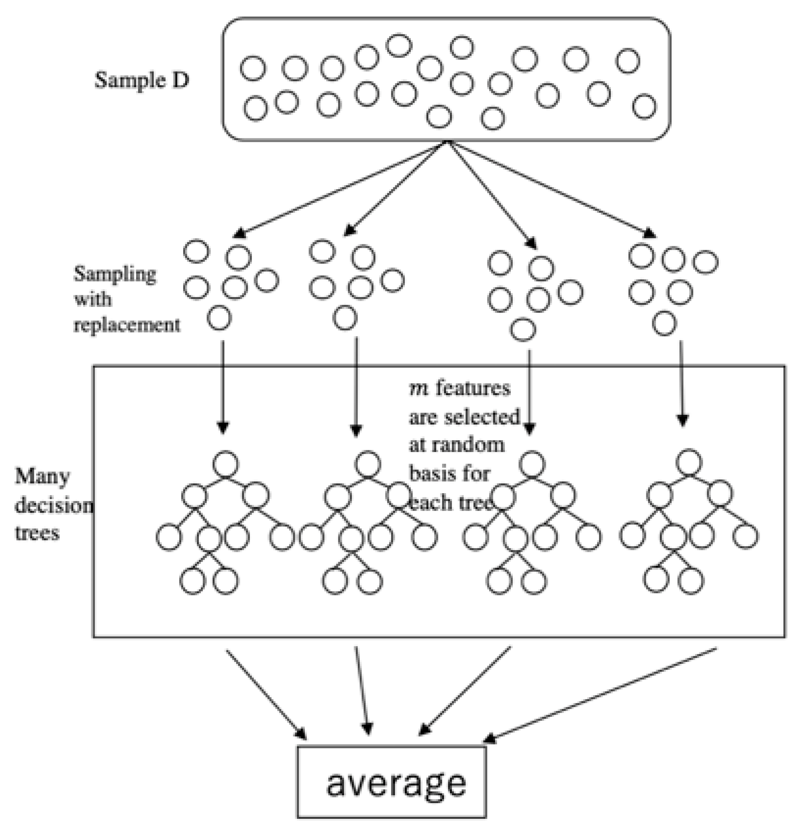
Random forest (Breiman 2001) is an ensemble learning method that builds multiple decision trees by analyzing data features and then merges them together to improve prediction performance. This method enables us to avoid an overfitting problem when more trees are added to the forest and improves prediction performance because each tree is drawn from the original sample using bootstrap resampling and is grown based on a randomly selected feature. The uncorrelated models obtained from this method improve prediction performance, as the feature mentioned above protects individual errors from each other. In this way, an individual error will not interfere with the entire group moving toward the correct direction. The random forest produces regression trees through the following steps (Figure 1):

Assume that there is a dataset $D=\left\{\left(x_1, y_1\right)\dots \dots \left(x_n,y_n\right)\right\}$ and the target is to find the function $f:X\to Y$, where $X$ is the inputs, and $Y$ is the produced outputs. Let $M$ be the number of features.

• Random forest randomly selects $n$ observations from the sample $D$ with a replacement to form a bootstrap sample.
• Multiple trees are grown by subsets of $m$ features from the overall $M$ features. For each subset, $m$ features are selected at random.

A prediction is produced by taking the average of the predictions from all trees in the forest (in the case of a classification problem, a prediction is decided by the majority).

In this paper, X indicates the fundamental economic features, and Y is the exchange rate. D refers to all data.

4.2. Support Vector Machine

The original SVM algorithm was introduced by Vapnik and Lerner (1963). Boser et al. (1992) suggested an alternative way to create nonlinear classifiers by applying the kernel functions to maximum-margin hyperplanes.

The primary concept of SVM regression is discussed first with a linear model and then is extended to a non-linear model using the kernel functions. Given the training data $\left\{\left(x_1,y_1\right), \dots , \left(x_1,y_1\right), XϵR^n, YϵR\right\}$, the SVM regression can be given by

$$f\left(x\right)=w^{\top }x+b, \omega ϵX, bϵR$$

(26)

$\xi$ is the insensitive loss function considered in SVM from the loss function described as

$${\left|\xi \right|}_{\epsilon }={|y-f(x\left)\right|}_{\epsilon }=\{\begin{array}{cc}0& if|y-f(x\left)\right|\le \epsilon \\ |y-f(x\left)\right|\le \epsilon & \mathit{otherwise}\end{array}.$$

(27)

The principal objective of SVM regression is to find function $f\left(x\right)$ with the minimum value of the loss function and also to make it as flat as possible. Thus, the model can be expressed as the following convex optimization problem:

$$\min \frac{1}{2}{\Vert w\Vert }^2+C\left({{\displaystyle \sum }}_i^l{\xi }_i^{*}+{{\displaystyle \sum }}_{i=1}^l{\xi }_i\right),$$

(28)

subject to

$$y_i-w^{\top }x-b\le \epsilon +{\xi }_i$$

(29)

$$w^{\top }x+b-y_i\le \epsilon +{\xi }_i^{*}$$

(30)

$${\xi }_i, {\xi }_i^{*}\ge 0$$

(31)

where C determines the trade-off between the flatness of $f\left(x\right)$ and the amount up to which deviations larger than $\epsilon$ are tolerable (${\xi }_i$,${\xi }_i^{*}$).

After solving the Lagrange function from Equations (29)–(31) and using the kernel function, the SVM model using the kernel function can be expressed as follows:

$$\max -\frac{1}{2}{{\displaystyle \sum }}_{i, j=1}^l({\alpha }_i-{\alpha }_i^{*})\left({\alpha }_j-{\alpha }_j^{*}\right)k\left(x_i,x_j\right)+{{\displaystyle \sum }}_{i=1}^l{y}_i\left({\alpha }_i-{\alpha }_i^{*}\right)-\epsilon {{\displaystyle \sum }}_{i=1}^l\left({\alpha }_i-{\alpha }_i^{*}\right)$$

(32)

subject to

$${{\displaystyle \sum }}_{i=1}^l\left({\alpha }_i-{\alpha }_i^{*}\right)=0,$$

(33)

$${\alpha }_i, {\alpha }_i^{*}ϵ \left[0,C\right].$$

(34)

where $k\left(x_i, x_j\right)$ is the kernel function, and ${\alpha }_i, {\alpha }_i^{*}$ are the Lagrangian multipliers. SVM can be performed by various functions, such as the linear, polynomial, or radial basis function (RBF), and sigmoid functions. This paper uses the radial basis function SVM model. The radial basis function can be expressed as follows:

$$k\left(x_i,x_j\right)=\exp \left(-\sigma {\left|x_i-x_j\right|}^2\right).$$

(35)

Here, the best C and sigma are determined using a grid search. Depending on the size of the C parameter, there is a trade-off between the correct classification of training examples and a smooth decision boundary. A larger C does not tolerate misclassification, offering a more complicated decision function, which a smaller C does tolerate. In this way, a simpler decision function is given. The sigma parameter defines how far the influence of a single training example reaches, with low values meaning ‘far’ and high values meaning ‘close’. A larger sigma gives a great deal of weight to the variables nearby, so the decision boundary becomes wiggly. For a smaller sigma, the decision boundary resembles a linear boundary, since it also takes distant variables into consideration.

4.3. Neural Network

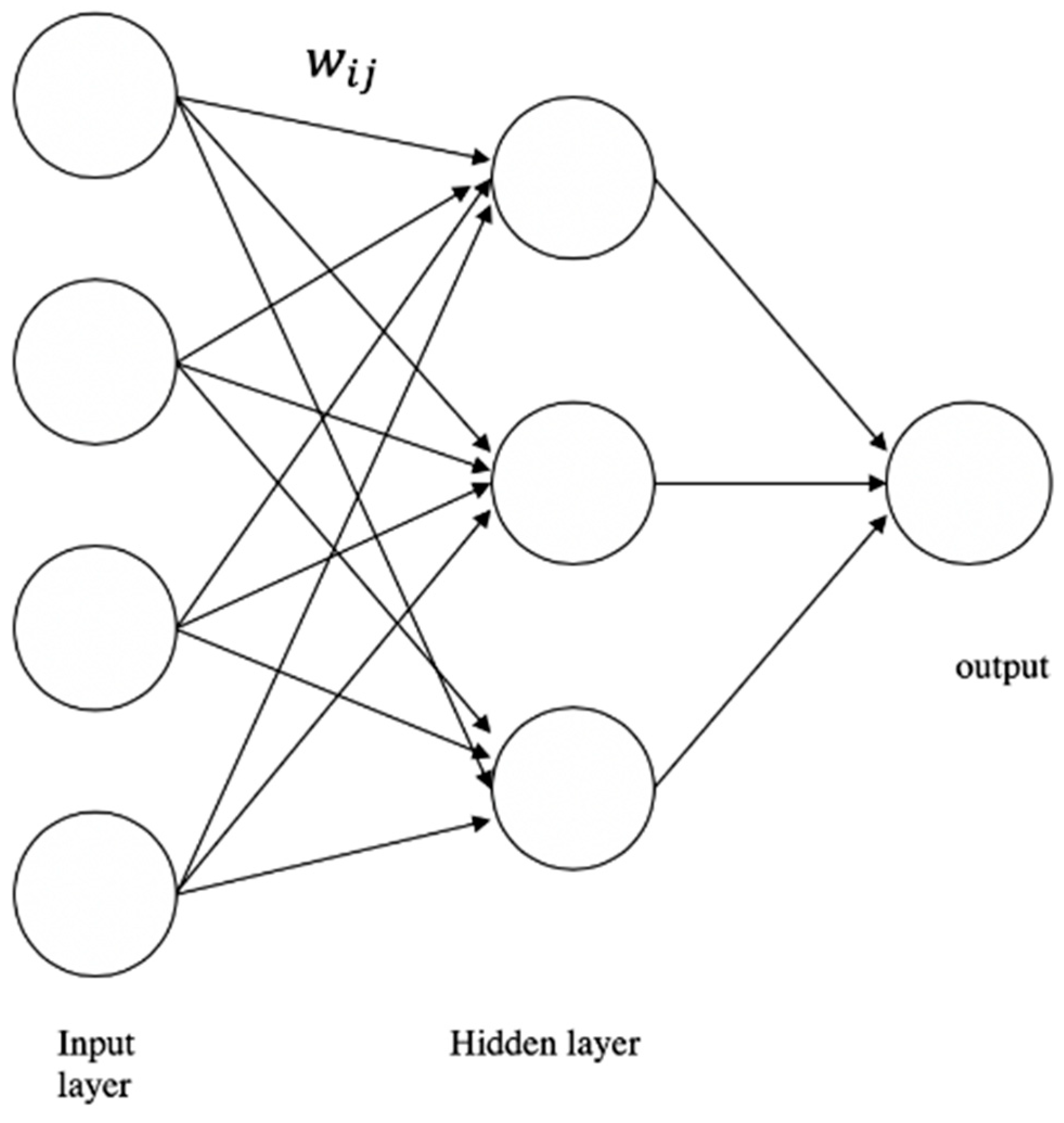
The feedforward neural network is the first and simplest type of neural network model. General references for this model include Bishop (1995), Hertz et al. (1991), and Ripley (1993, 1996). This paper uses one hidden layer model, which is the simplest model, as shown in Figure 2.

As shown in Figure 2, the information moves forward from the input nodes, through the hidden nodes, and then reaches the output nodes.

Inputs are summed by individual nodes. Then, adding a bias ($w_{ij}$ in the Figure 2), the result is substituted into a fixed function ${\varphi }_h$ (Equation (37)). The results of the output units are produced in the same process with output function ${\varphi }_o$. Thus, the equation of a neural network is written as follows:

$$y_k={\varphi }_o\left({\alpha }_k+{\displaystyle \sum }_h{w}_{hk}{\varphi }_h\left({\alpha }_h+{\displaystyle \sum }_i{w}_{ih}{x}_i\right)\right).$$

(36)

The activation function ${\varphi }_h$ of the hidden layer units usually takes a logistic function as

$$l\left(z\right)=\frac{1}{1+e^{-z}},$$

(37)

and the output function ${\varphi }_o$ usually takes a linear function in regression (in the case of a classification problem, the output function often takes a logistic form.)

Here, we adjust two hyper-parameters, which are the number of the units in the hidden layer C and the parameter for weight decay, using a grid search. The latter is a regularization parameter to avoid the over-fitting problem (Venables and Ripley 2002).

5. Results and Evaluation

5.1. Root Mean Squared Error

Random walk uses the following equation:

$${\left\{{\displaystyle \sum }_{s=0}^{46}{[\mathrm{A}\left(\mathrm{t}+\mathrm{s}+1\right)-\mathrm{A}\left(\mathrm{t}+\mathrm{s}\right)]}^2/47\right\}}^{\frac{1}{2}}.$$

(38)

For the other machine learning models, the following equation is used:

$$\begin{array}{c}{\left\{{\displaystyle {\displaystyle \sum }_{s=0}^{46}}{[\mathrm{F}\left(\mathrm{t}+\mathrm{s}+1\right)-\mathrm{A}\left(\mathrm{t}+\mathrm{s}+1\right)]}^2/47\right\}}^{\frac{1}{2}}\end{array}$$

(39)

where $A\left(t\right)$ denotes the actual value of the change rate in the exchange rate, and $F\left(t\right)$ is the predicted value. If $S=0$, then $S$ is a prediction for September 2015.

5.2. Modified Diebold–Mariano Test

The DM test was proposed by Diebold and Mariano (1995). This test examines whether the null hypothesis (that the competing model has the same predictive accuracy) is statistically true. Let us define the forecast error $e_{it}$ as

$$e_{it}={\widehat{y}}_{\mathrm{it}}-y_t,i=1,2$$

(40)

where ${\widehat{y}}_{\mathrm{it}} \mathrm{and} y_t$ are the predicted and actual values at time t, respectively.

Let $\mathrm{g}\left(e_{it}\right)$ denote the loss function. In this paper, it is defined as the following

$$g\left(e_{it}\right)=e_{it}^2.$$

(41)

Then, the loss differential $d_t$ can be written as

$$d_t=g\left(e_{1t}\right)-g\left(e_{2t}\right).$$

(42)

The statistic for the DM test is defined as follows:

$$\mathrm{DM}=\frac{\overline{d}}{\sqrt{\frac{s}{N}}}$$

(43)

where $\overline{d}$, $s$, and $N$ represent the sample mean, the variance of $d_t$, and the sample size, respectively. The null hypothesis is that ${\mathrm{H}}_0:\mathrm{E}\left[d_t\right]=0 \forall t$, which means that the two forecasts have the same accuracy, while the alternative hypothesis is that ${\mathrm{H}}_1: E\left[d_t\right]\ne 0 \forall t$, meaning that the two forecasts have different levels of accuracy. If the null hypothesis is true, then the DM statistic is asymptotically distributed as N(0, 1), the standard normal distribution.

A modified DM test was proposed by Harvey et al. (1997), who found that the modified DM test performs better than the original one. They defined the statistic for the modified DM test as follows:

$$D{M}^{*}={\left[\frac{n+1-2h+n^{-1}h\left(h-1\right)}{n} \right]}^{\frac{1}{2}}DM$$

(44)

where $h$ denotes the horizon, and the DM represents the original statistic, as in Equation (43). In this study, we predict one period ahead, meaning that $h=1$, so $D{M}^{*}={\left(\frac{n-1}{n}\right)}^{\frac{1}{2}}DM$.

Table 2. Results for the uncovered interest rate parity (UIRP) model.

Features	Evaluation	Random Forest	SVM	Neural Network	Random Walk
bond_1y	RMSE	2.842	2.552	2.516	3.552
	DM	−2.101	−2.481	−2.515
	p-value	0.02	0.008	0.008
bond_2y	RMSE	3.391	2.495	2.525	3.552
	DM	−0.391	−2.496	−2.520
	p-value	0.349	0.008	0.008
bond_3y	RMSE	3.011	2.578	2.509	3.552
	DM	−0.886	−2.500	−2.512
	p-value	0.19	0.008	0.008
bond_5y	RMSE	3.151	2.636	2.489	3.552
	DM	−0.997	−2.508	−2.595
	p-value	0.162	0.008	0.006
bond_7y	RMSE	2.769	2.478	2.517	3.552
	DM	−1.725	−2.527	−2.557
	p-value	0.046	0.007	0.007
bond_10y	RMSE	2.856	2.525	2.525	3.552
	DM	−1.809	−2.565	−2.539
	p-value	0.038	0.007	0.007

Note. “UIRP” indicates uncovered interest rate parity, “SVM” indicates support vector machine, “DM” indicates the modified Diebold–Mariano test statistic as in Equation (44), “bond_1y” indicates the government bond with 1 year to maturity. “bond_2y” indicates the government bond with two years to maturity. “bond_3y” indicates the government bond with three years to maturity. “bond_5y” indicates the government bond with five years to maturity. “bond_7y” indicates the government bond with seven years to maturity. “bond_10y” indicates the government bond with ten years to maturity.

,

Table 3. Results for the purchasing power parity (PPP) model.

Features	Evaluation	Random Forest	SVM	Neural Network	Random Walk
PPP_PPI	RMSE	2.759	2.493	2.469	3.552
	DM	−1.771	−2.632	−2.652
	p-value	0.042	0.006	0.005
PPP_CPI	RMSE	3.187	2.528	2.510	3.552
	DM	−0.870	−2.633	−2.576
	p-value	0.194	0.006	0.007
PPP_CPI_CORE	RMSE	2.554	2.561	2.516	3.552
	DM	−2.340	−2.566	−2.568
	p-value	0.012	0.007	0.007
PPP_CPI_CORECORE	RMSE	3.303	2.533	2.508	3.552
	DM	−0.744	−2.541	−2.580
	p-value	0.230	0.007	0.007

Note. “PPP” indicates purchasing power parity, “DM” indicates modified Diebold–Mariano test statistic as in Equation (44), “PPI” indicates producer price index, “CPI” indicates the CPI of all items, “CPI_CORE” indicates the CPI excluding fresh food, and “CPI_CORECORE” indicates the CPI excluding fresh food and energy.

,

Table 4. Results for the monetary model.

Features	Evaluation	Random Forest	SVM	Neural Network	Random Walk
monetary_PPI	RMSE	2.619	2.530	2.514	3.552
	DM	−2.203	−2.588	−2.639
	p-value	0.016	0.006	0.006
monetary_CPI	RMSE	2.960	2.647	2.530	3.552
	DM	−1.622	−2.472	−2.541
	p-value	0.056	0.009	0.007
monetary_CPI_CORE	RMSE	2.817	2.479	2.535	3.552
	DM	−1.895	−2.192	−2.518
	p-value	0.032	0.005	0.008
monetary_CPI_CORECORE	RMSE	2.899	2.614	2.515	3.552
	DM	−1.723	−2.467	−2.566
	p-value	0.046	0.009	0.007

Note. “DM” indicates modified Diebold–Mariano test statistic, as in Equation (44), “PPI” indicates producer price index, “CPI” indicates the CPI of all items, “CPI_CORE” indicates the CPI excluding fresh food, and “CPI_CORECORE” indicates the CPI excluding fresh food and energy.

,

Table 5. Results for the Taylor model (Equation (25)).

Features	Evaluation	Random Forest	SVM	Neural Network	Random Walk
Taylor1_PPI	RMSE	2.515	2.493	2.492	3.552
	DM	−2.457	−2.620	−2.666
	p-value	0.009	0.006	0.005
Taylor1_CPI	RMSE	2.822	2.544	2.523	3.552
	DM	−2.142	−2.612	−2.565
	p-value	0.019	0.006	0.007
Taylor1_CPI_CORE	RMSE	2.785	2.473	2.504	3.552
	DM	−2.136	−2.649	−2.559
	p-value	0.019	0.006	0.007
Taylor1_CPI_CORECORE	RMSE	2.683	2.557	2.520	3.552
	DM	−2.131	−2.503	−2.529
	p-value	0.019	0.008	0.007

Note. “SVM” indicates support vector machine, “DM” indicates modified Diebold–Mariano test statistic as in Equation (44), “Taylor1” indicates using Equation (25), “PPI” indicates producer price index, “CPI” indicates the CPI of all items, “CPI_CORE” indicates the CPI excluding fresh food, and “CPI_CORECORE” indicates the CPI excluding fresh food and energy.

and

Table 6. Result for the Taylor model (Equation (24)).

Features	Evaluation	Random Forest	SVM	Neural Network	Random Walk
Taylor2_PPI_2y	RMSE	2.564	2.492	2.499	3.552
	DM	−2.312	−2.512	−2.440
	p-value	0.013	0.008	0.009
Taylor2_PPI_3y	RMSE	2.541	2.491	2.468	3.552
	DM	−2.263	−2.522	−2.554
	p-value	0.014	0.008	0.007
Taylor2_PPI_5y	RMSE	2.498	2.482	2.497	3.552
	DM	−2.563	−2.537	−2.517
	p-value	0.007	0.007	0.008
Taylor2_PPI_7y	RMSE	2.455	2.464	2.522	3.552
	DM	−2.601	−2.547	−2.435
	p-value	0.006	0.007	0.009
Taylor2_PPI_10y	RMSE	2.457	2.451	2.537	3.552
	DM	−2.556	−2.584	−2.518
	p-value	0.007	0.006	0.008
Taylor2_CPI_2y	RMSE	2.733	2.554	2.513	3.552
	DM	−2.149	−2.495	−2.564
	p-value	0.018	0.008	0.007
Taylor2_CPI_3y	RMSE	2.664	2.559	2.525	3.552
	DM	−2.211	−2.492	−2.534
	p-value	0.016	0.008	0.007
Taylor2_CPI_5y	RMSE	2.661	2.544	2.491	3.552
	DM	−2.274	−2.541	−2.597
	p-value	0.014	0.007	0.006
Taylor2_CPI_7y	RMSE	2.687	2.537	2.507	3.552
	DM	−2.223	−2.557	−2.559
	p-value	0.016	0.007	0.007
Taylor2_CPI_10y	RMSE	2.652	2.548	2.500	3.552
	DM	−2.333	−2.576	−2.550
	p-value	0.012	0.007	0.007
Taylor2_CPI_CORE_2y	RMSE	2.670	2.501	2.525	3.552
	DM	−2.193	−2.476	−2.537
	p-value	0.017	0.009	0.007
Taylor2_CPI_CORE_3y	RMSE	2.736	2.502	2.513	3.552
	DM	−2.083	−2.495	−2.567
	p-value	0.021	0.008	0.007
Taylor2_CPI_CORE_5y	RMSE	2.552	2.488	2.523	3.552
	DM	−2.500	−2.536	−2.541
	p-value	0.008	0.007	0.007
Taylor2_CPI_CORE_7y	RMSE	2.575	2.468	2.509	3.552
	DM	−2.312	−2.587	−2.574
	p-value	0.013	0.006	0.007
Taylor2_CPI_CORE_10y	RMSE	2.471	2.486	2.512	3.552
	DM	−2.677	−2.588	−2.564
	p-value	0.005	0.006	0.007
Taylor2_CPI_CORECORE_2y	RMSE	2.601	2.547	2.543	3.552
	DM	−2.194	−2.423	−2.438
	p-value	0.017	0.01	0.009
Taylor2_CPI_CORECORE_3y	RMSE	2.622	2.542	2.494	3.552
	DM	−2.160	−2.447	−2.601
	p-value	0.018	0.009	0.006
Taylor2_CPI_CORECORE_5y	RMSE	2.565	2.531	2.533	3.552
	DM	−2.296	−2.499	−2.478
	p-value	0.013	0.008	0.008
Taylor2_CPI_CORECORE_7y	RMSE	2.618	2.521	2.532	3.552
	DM	−2.171	−2.505	−2.470
	p-value	0.018	0.008	0.009
Taylor2_CPI_CORECORE_10y	RMSE	2.505	2.525	2.492	3.552
	DM	−2.530	−2.545	−2.555
	p-value	0.007	0.007	0.007

Note. “SVM” indicates support vector machine, “Taylor2” indicates using Equation (24), “DM” indicates modified Diebold–Mariano test statistic as in Equation (44), “PPI” indicates producer price index, “CPI” indicates the CPI of all items, “CPI_CORE” indicates the CPI excluding fresh food, and “CPI_CORECORE” indicates the CPI excluding fresh food and energy. “Taylor2_PPI_2y” indicates using the PPI to calculate the inflation rate and using a government bond with 2 year to maturity to calculate the lagged interest rate. “bond_2y” indicates the government bond with two years to maturity. “bond_3y” indicates the government bond with three years to maturity. “bond_5y” indicates the government bond with five years to maturity. “bond_7y” indicates the government bond with seven years to maturity. “bond_10y” indicates the government bond with ten years to maturity.

indicate the following. According to the RMSE, the fundamental models using machine learning outperform the random walks with regard to their error size. This is also confirmed by the MAPE (Appendix A,

Table A1. Mean absolute percentage error (MAPE) of UIRP Model.

Features	Random Forest	SVM	Neural Network	Random Walk
bond_1y	2.276	1.767	1.772	2.768
bond_2y	2.672	1.770	1.781	2.768
bond_3y	2.269	1.768	1.765	2.768
bond_5y	2.442	1.765	1.750	2.768
bond_7y	2.106	1.767	1.769	2.768
bond_10y	2.036	1.772	1.772	2.768

Note. “UIRP” indicates uncovered interest rate parity, “SVM” indicates support vector machine, “bond_1y” indicates the government bond with 1 year to maturity. “bond_2y” indicates the government bond with two years to maturity. “bond_3y” indicates the government bond with three years to maturity. “bond_5y” indicates the government bond with five years to maturity. “bond_7y” indicates the government bond with seven years to maturity. “bond_10y” indicates the government bond with ten years to maturity.

). Since this is confirmed regardless of the government bonds’ time to maturity and the price level measurements used, these findings are robust. Furthermore, models using PPI always show better predictability compared to CPI. This empirical result is in line with that of Hashimoto (2011). Because of the close trading relationship between Japan and the US, the fluctuation of JPY/USD tends to be influenced by PPI rather than CPI. The poor performance of CPI in terms of its error size and the significance of its predictive accuracy could be explained by the inclusion of volatile price indicators, such as food, beverages, and energy, w makes it difficult to measure an accurate inflation rate gap. In addition, in the case of the Taylor rule models, both Equations (24) and (25) present reasonable results for this empirical study. This demonstrates that either equation can be used to predict the exchange rate.

From the perspective of the modified DM test, we can see that most of the results show significantly different predictive accuracies compared to the random walk, while some of the random forest results show the same predictive accuracy as the random walk. Random forest is a weak tool for predicting the out-of-sample exchange rate compared with the other machine learning models. This seems reasonable, as the random forest model ignores two characteristics of time series data, that is, inherent time trend and the interdependency among variables. However, random forest can be useful in predicting time series data in some cases, such as that in Dudek (2015).

6. Conclusions

Since the work of Meese and Rogoff (1983a, 1983b), there have been many attempts by researchers to solve the puzzle of why traditional economical models are not able to outperform the random walk in predicting out-of-sample exchange rates. In recent years, Amat et al. (2018) found that in combination with machine learning methodologies, traditional exchange-rate models and Taylor-rule exchange rate models can be useful for forecasting future short-term exchange rates across 12 major currencies.

In this paper, we analyzed whether combining modern machine learning methodologies with economic models could outperform the prediction performance of a random walk without drift. More specifically, this paper sheds light on the application of the random forest method, the support vector machine, and neural networks to four fundamental theories (uncovered interest rate parity, purchase power parity, the monetary model, and the Taylor rule models). The robustness of the results was also thoroughly examined using six government bonds with different maturities and four different price indexes in three machine learning models. This provides concrete evidence for predictive performance.

In the empirical analysis, a rolling window analysis was used for the one-period-ahead forecast for JPY/USD. Using sample data from between August 1980 and August 2019, there were two main findings. First, comparing the performance of the fundamental models combining machine learning with the performance obtained by the random walk, the RMSE results show that the former models outperform the random walk. In the DM test, most of the results show a significantly different predictive accuracy with the random walk, while some of the random forest results show the same accuracy as the random walk. Second, comparing the performance of the fundamental models combined with machine learning, the models using PPI show fairly good predictability in a consistent manner, from the perspective of both the size of their errors and their predictive accuracy. However, CPI does not appear to be a useful index for predicting exchange rate based on its poor results in the RMSE test and DM test.

References

1. Amat, Christophe, Tomasz Michalski, and Gilles Stoltz. 2018. Fundamentals and exchange rate forecastability with machine learning methods. Journal of International Money Finance 88: 1–24. [Google Scholar] [CrossRef]
2. Bishop, Christopher M. 1995. Neural Networks for Pattern Recognition. Oxford: Oxford University Press. [Google Scholar]
3. Boser, Bernhard E., Isabelle M. Guyon, and Vladimir N. Vapnik. 1992. A training algorithm for optimal margin classifiers. In Proceedings of the Fifth Annual Workshop of Computational Learning Theory, Pittsburg, PA, USA, 27–29 July 1992; New York: ACM, Volume 5, pp. 144–52. [Google Scholar]
4. Breiman, Leo. 2001. Random Forests. Machine Learning 45: 5–32. [Google Scholar] [CrossRef] [Green Version]
5. Cassel, Karl Gustav. 1918. Abnormal Deviations in International Exchanges. Economic Journal 28: 413–15. [Google Scholar] [CrossRef] [Green Version]
6. Cervelló-Royo, Roberto, Francisco Guijarro, and Karolina Michniuk. 2015. Stock market trading rule based on pattern recognition and technical analysis: Forecasting the DJIA index with intraday data. Expert System with Applications 42: 5963–75. [Google Scholar] [CrossRef]
7. Chang, Pei-Chann, Di-di Wang, and Chang-Le Zhou. 2012. A novel model by evolving partially connected neural network for stock price trend forecasting. Expert Systems with Applications 39: 611–20. [Google Scholar] [CrossRef]
8. Cheung, Yin-Wong, Menzie D. Chinn, and Antonio Garcia Pascual. 2005. Empirical exchange rate models of the nineties: Are any fit to survive? Journal of International Money and Finance 24: 1150–75. [Google Scholar] [CrossRef] [Green Version]
9. Chong, Eunsuk, Chulwoo Han, and Frank C. Park. 2017. Deep learning networks for stock market analysis and prediction: Methodology, data representations, and case studies. Expert Systems with Application 83: 187–205. [Google Scholar] [CrossRef] [Green Version]
10. Clarida, Richard, Jordi Gali, and Mark Gertler. 1998. Monetary rules in practice: Some international evidence. European Economic Review 42: 1033–67. [Google Scholar] [CrossRef] [Green Version]
11. Diebold, Francis X., and Roberto S. Mariano. 1995. Comparing predictive accuracy. Journal of Business and Economic Statistics 13: 253–63. [Google Scholar]
12. Dudek, Grzegorz. 2015. Short-Term Load Forecasting Using Random Forests. In Intelligent Systems’2014. Advances in Intelligent Systems and Computing. Edited by Dimitar P. Filev. Cham: Springer, Volume 323. [Google Scholar]
13. Engel, Charles, and Kenneth D. West. 2005. Exchange rate and fundamentals. Journal of Political Economy 113: 485–517. [Google Scholar] [CrossRef] [Green Version]
14. Engel, Charles, and Kenneth D. West. 2006. Taylor rules and the Deutschmark-dollar real exchange rates. Journal of Money, Credit and Banking 38: 1175–94. [Google Scholar] [CrossRef] [Green Version]
15. Engel, Charles, Dohyeon Lee, Chang Liu, Chenxin Liu, and Steve Pak Yeung Wu. 2019. The uncovered interest parity puzzle, exchange rate forecasting, and Taylor rules. Journal of International Money and Finance 95: 317–31. [Google Scholar] [CrossRef] [Green Version]
16. Fisher, Irving. 1896. Appreciation and Interest. New York: Macmillan for the American Economic Association, Reprinted in The Works of Irving Fisher. Edited by William J. Barber. London: Pickering & Chatto, Volume 1. [Google Scholar]
17. Frenkel, Jacob A. 1976. Monetary Approach to the Exchange Rate: Doctrinal Aspects and Empirical Evidence. Scandinavian Journal of Economics 78: 200–24. [Google Scholar] [CrossRef]
18. García, Fernando David, Francisco Guijarro, Javier Oliver, and Rima Tamošiūnienė. 2018. Hybrid fuzzy neural network to predict price direction in the German DAX-30 index. Technological and Economic Development of Economy 24: 2161–78. [Google Scholar] [CrossRef]
19. Giacomini, Raffaela, and Barbara Rossi. 2010. Forecast Comparisons in Unstable Environments. Journal of Applied Econometrics 25: 595–620. [Google Scholar] [CrossRef]
20. Hamori, Shigeyuki, Minami Kawai, Takahiro Kume, Yuji Murakami, and Chikara Watanabe. 2018. Ensemble Learning or Deep Learning? Application to Default Risk Analysis. Journal of Risk and Financial Management 11: 12. [Google Scholar] [CrossRef] [Green Version]
21. Harvey, David, Stephen Leybourne, and Paul Newbold. 1997. Testing the equality of prediction mean squared errors. International Journal of Forecasting 13: 281–91. [Google Scholar] [CrossRef]
22. Hashimoto, Jiro. 2011. How well can the time series models forecast exchange rate changes? Bulletin of Niigata Sangyo University Faculty of Economics 39: 11–26. (In Japanese). [Google Scholar]
23. Hertz, John A., Anders S. Krogh, and Richard G. Palmer. 1991. Introduction to the Theory of Neural Computation. Boulder: Westview Press. [Google Scholar]
24. Jamali, Ibrahim, and Ehab Yamani. 2019. Out-of-sample exchange rate predictability in emerging markets: Fundamentals versus technical analysis. Journal of International Financial Markets, Institutions and Money 61: 241–63. [Google Scholar] [CrossRef]
25. Mark, Nelson C. 1995. Exchange Rates and Fundamentals: Evidence on Long-Horizon Predictability. The American Economic Review 85: 201–18. [Google Scholar]
26. Meese, Richard A., and Kenneth S. Rogoff. 1983a. Empirical Exchange Rate Models of the Seventies: Do They Fit Out of Sample? Journal of International Economics 14: 3–24. [Google Scholar] [CrossRef]
27. Meese, Richard A., and Kenneth Saul Rogoff. 1983b. The out-of-sample failure of empirical exchange rate models: Sampling error or mis-specification? In Exchange Rates and International Macroeconomics. Edited by Jacob Frenkel. Chicago: NBER and University of Chicago Press. [Google Scholar]
28. Molodtsova, Tanya, and David H. Papell. 2009. Out-of-Sample Exchange Rate Predictability with Taylor Rule Fundamentals. Journal of International Economics 77: 167–80. [Google Scholar] [CrossRef]
29. Mussa, Michael. 1976. A Model of Exchange Rate Dynamics. Scandinavian Journal of Economics 78: 229–48. [Google Scholar] [CrossRef]
30. Ripley, Brian D. 1993. Statistical Aspects of neural networks. In Networks on Chaos: Statistical and Probabilistic Aspects. Edited by Ole Eiler Barndorff-Nielsen, J. L. Jensen and Wilfrid S. Kendall. London: Chapman & Hall, pp. 40–123. [Google Scholar]
31. Ripley, Brian D. 1996. Pattern Recognition and Neural Networks. Cambridge: Cambridge University Press. [Google Scholar]
32. Rossi, Barbara. 2013. Exchange Rate Predictability. Journal of Economic Literature 51: 1063–119. [Google Scholar] [CrossRef] [Green Version]
33. Taylor, John B. 1993. Discretion versus policy rules in practice. Carnegie-Rochester Conference Series on Public Policy 39: 195–214. [Google Scholar] [CrossRef]
34. Taylor, Mark P. 1995. The economics of exchange rate. Journal of Economic Literature 33: 13–47. [Google Scholar]
35. Vapnik, Vladimir N., and A. Lerner. 1963. Pattern recognition using generalized portrait method. Automation and Remote Control 24: 774–80. [Google Scholar]
36. Venables, William N., and Brian D. Ripley. 2002. Modern Applied Statistics with S, 4th ed. New York: Springer, pp. 243–45. [Google Scholar]
Figure 1. Mechanism of random forest.
Jrfm 13 00048 g001
Figure 2. The mechanism of a neural network.
Jrfm 13 00048 g002