Article

Dynamic Bankruptcy Prediction Models for European Enterprises

Faculty of Management and Economics, Gdansk University of Technology, Narutowicza 11/12, 80-233 Gdansk, Poland
J. Risk Financial Manag. 2019, 12(4), 185; https://doi.org/10.3390/jrfm12040185
Submission received: 8 November 2019 / Revised: 4 December 2019 / Accepted: 5 December 2019 / Published: 9 December 2019
(This article belongs to the Special Issue Modern Methods of Bankruptcy Prediction)

Abstract

:
This manuscript is devoted to the issue of forecasting corporate bankruptcy. Determining a firm’s bankruptcy risk is one of the most interesting topics for investors and decision-makers. The aim of the paper is to develop and to evaluate dynamic bankruptcy prediction models for European enterprises. To conduct this objective, four forecasting models are developed with the use of four different methods—fuzzy sets, recurrent and multilayer artificial neural network, and decision trees. Such a research approach will answer the question of whether changes in indicators are relevant predictors of a company’s coming financial crisis because declines or increases in values do not immediately indicate that the company’s economic situation is deteriorating. The research relies on two samples of firms—the learning sample of 50 bankrupt and 50 non-bankrupt enterprises and the testing sample of 250 bankrupt and 250 non-bankrupt firms.

1. Introduction

The measurement of corporate bankruptcy risk is one of the major challenges of modern economic and financial research. Nowadays, with increased financial globalization, faster economic changes, and a new dimension of increased financial risk in the context of the global financial crisis that arose since 2007, we should focus on increasing the reliability of the forecasting model and on prolonging the forecasting horizon to even 10 years prior to announcement of bankruptcy.
The consequences of financial failure are enormous for financial creditors, managers, shareholders, investors, employees, and even a country’s economy. That is why during the past five decades, predicting corporate bankruptcy has become a significant concern for the various stakeholders in firms. Accurate bankruptcy prediction usually leads to many benefits, such as cost reduction in credit analysis, better monitoring, and an increased debt-collection rate. Thus, bankruptcy forecasting has become of major interest and is gaining much more importance currently. Today, the question is not if we should use bankruptcy forecasting models, but how to increase the effectiveness of forecasting models.
Though the first law on bankruptcy was already written in 1542 in England during the reign of King Henry VIII, the first studies on forecasting bankruptcies took place in the 1960s, started by Beaver (1966) and Altman (1968). There are two main distinct strands of models that have been used to predict bankruptcy—statistical and artificial intelligence models.
Since the estimation of the pioneering model of multivariate discriminant analysis by Altman, numerous research studies have been carried out with the use of a wide variety of statistical methods (e.g., Alaka et al. 2018; Bandyopadhyay 2006; Barboza et al. 2017; Delen et al. 2013; Giannopoulos and Sigbjornsen 2019; Ho et al. 2013; Hosmer et al. 2013; Jackson and Wood 2013; Kieschnick et al. 2013; Kumar and Ravi 2007; Laitinen 2007; Lukason and Hoffman 2014; Lyandres and Zhdanov 2013; Mihalovic 2016; Orsenigo and Vercellis 2013; Psillaki et al. 2010). The most popular statistical techniques as noted by Balcaen and Ooghe (2006) are multivariate discriminant analysis and logistic regression models.
Although the statistical techniques have become the most commonly used in bankruptcy prediction, they are characterized by many disadvantages regarding statistical assumptions, such as linearity, normality, and independence among variables, which have been identified in many studies (e.g., Altman 2018; Balcaen and Ooghe 2006; Jardin and Severin 2011; Tian and Yu 2017; Jayasekera 2018). That is why in the last two decades, popularity of bankruptcy prediction methods has shifted from statistical to intelligent ones such as neural networks, genetic algorithms, vector support machines, fuzzy logic (e.g., Acosta-González and Fernández-Rodríguez 2014; Ahn et al. 2000; Andres et al. 2005; Atiya 2001; Brabazon and O’Neil 2004; Callejon et al. 2013; Dong et al. 2018; Garcia et al. 2019; Hosaka 2019; Jardin 2015; Jardin 2018; Kim and Kang 2010; Lensberg et al. 2006; Lin et al. 2014; Min and Lee 2005; Ptak-Chmielewska 2019; Ravisankar and Ravi 2010; Succurro et al. 2019; Sun et al. 2014; Tam 1991; Tsai 2014; Wu et al. 2010; Zapranis and Ginoglou 2000; Xiao et al. 2012). The most popular method, which has been in use since the 1990s, is neural networks.
A detailed analysis of the literature on bankruptcy prediction shows that since the first studies, the main concern in the literature was to assess which method was the most effective in making predictions. Though many novel sophisticated techniques have been proposed for effective prediction, the majority of models ensure optimal predictive ability when the forecasting horizon is short, and their accuracy decreases severely beyond three years. Regardless of the modeling technique (linear or non-linear, regression or classification), most models are based on a static snapshot of financial situation that is static values of financial ratios for a given moment of time (usually at the end of the year). These models lack a dynamic approach to indicators. The question arises whether changes in indicators are relevant predictors of a company’s coming financial crisis because declines or increases in values do not immediately indicate that the company’s economic situation is deteriorating. Nevertheless, by observing changes, we can distinguish between a company that has low financial ratios that improve each year and a company that has similarly low ratios that worsen each year. Static models will not detect the difference between such companies. Dynamic models can add an element that differentiates companies with a poor financial situation from companies that have a weak financial situation but are improving.
To answer this research question, the main objective of this study is to develop dynamic bankruptcy prediction models for European enterprises with the use of four methods—fuzzy sets, artificial neural networks (multilayer and recurrent), and decision trees. This paper, therefore, makes three major contributions to the bankruptcy prediction literature. First, it implements a dynamic approach to financial ratios describing the economic situation of enterprises. Second, it verifies the influence of the dynamic approach on effectiveness of models developed with the use of four different forecasting techniques. Third, it allows the analysis of which method has the smallest decrease in effectiveness in extending the forecast horizon from one to 10 years. Very few studies in the literature focus on this crucial aspect. By evaluating and identifying the predictive properties of models in longer forecasting periods, we can build a decision-support model that will give managers more time in the decision-making process and thus prevent bankruptcies.
The paper consists of five sections. In the Introduction, the author justifies the topic, the study objectives, and the contributions and innovations to the literature. Section 2 presents an overview of the limitations of bankruptcy prediction models. Section 3 introduces this study’s assumptions. In Section 4, the author presents four bankruptcy prediction models and discusses the results of effectiveness tests. Section 5 concludes the paper.

2. Literature Review

A thoughtful review on limitations of bankruptcy prediction models is useful to help readers understand the research and the appropriate process of estimation of forecasting models.
The first discussion point is the definition of financial distress. The purpose of bankruptcy forecasting models should be early recognition that the company will be threatened with bankruptcy. From a methodological point of view, it is important to define the term “bankruptcy”. In the literature, there are various definitions. The most common interpretation of “bankruptcy” is the criterion of the insolvency of the company. The insolvency is understood as the inability to pay debts (e.g., Crone and Finlay 2012; Deakin 1972; Foster 1986; Jardin 2017). If a company is not able to honor its short-term debt, it is considered to be technically insolvent. Technical insolvency indicates a lack of liquidity but does not yet determine the bankruptcy of the company. Lack of ability to pay current liabilities may be temporary and can be remedied by appropriate action of company management. Altman, a world authority on bankruptcy issues, finds that insolvency understood as a cause of bankruptcy is a long-term state in which the business is found if its total debt exceeds the value of all assets held (Altman 1968). In the studies of Doumpos and Zopounidis (Doumpos and Zopounidis 1999), financial distress not only contains inability to repay important obligatory payments, but also includes the situation of negative net asset value, which means an enterprise’s total liabilities exceed its total assets from the view of accounting.
On the other hand, Berryman (1992) suggests a profitability criterion to define a company at risk of bankruptcy. According to him, “a company at risk of bankruptcy” is characterized by a lower long-term return on equity from the level of profitability possible to obtain in similar companies. However, such a wide interpretation of the term “bankruptcy” seems to be too broad. Even more so since research conducted by Davies (1997) on the fallen companies in the UK and France has revealed that most failed companies had positive financial results in the period preceding their bankruptcy.
An equally broad and controversial interpretation of the concept of corporate bankruptcies was presented by Watson and Everett (1999), who stated that a simple change of the owners of the company is a form of failure. In literature, the term “financial failure” is often used interchangeably with the term “bankruptcy”. The criterion of continuity of ownership in the company seems to be a too far-fetched over-interpretation of the term “bankruptcy”.
The second issue concerns an assessment of the effectiveness of the statistical bankruptcy prediction models such as the multivariate discriminant analysis and the logit and probit models. The allegation concerns the ability to manipulate the thresholds of these models in order to maximize the results of the classification of models. This objection is raised by Nwogugu (2007), according to whom statistical methods do not provide reliable results due to the ease of manual adjustment of the threshold so as to increase the effectiveness of the model. Such manipulation, of course, will not increase the effectiveness of the model in the general population of companies after implementation of the model, e.g., in a bank, but only in the given testing sample of the author of the model.
Another shortcoming of traditional forecasting models is their stationarity (e.g., Balcaen and Ooghe 2006; Grice and Dugan 2001; Liang et al. 2016; Mensah 1984). Bankruptcy models are usually estimated with the use financial ratios calculated with data from balance sheets and income statements. The use of ratios is as much due to their predictive power as to their availability and standardization (Jardin 2016). They generally allow for good discrimination between failed and non-failed firms. However, the way they are designed is one of their main weaknesses. The majority of the models are developed based on static values of financial ratios for a given moment of time, but bankruptcy has multiple causes and symptoms, and a model with variables that are solely measured over a single period would probably not be able to embody such diversity. The financial crisis in enterprise is a dynamic process, and it does not depend on the sole situation of a firm at a given period but is the result of many factors that often overlap. The ability of a model to capture the whole variety of negative situations is a key factor of its performance. As mentioned before, this raises the question of whether changes in the indicators are relevant predictors of the upcoming financial crisis in the company. The dynamic approach to financial ratios could help to introduce an additional element discriminating companies at risk of bankruptcy from enterprises that are in bad financial condition but improving, that is distancing them from the risk of going bankrupt. These considerations are part of the empirical analysis in next sections of the paper.
The next accusation against bankruptcy forecasting models is the issue of their obsolescence with the passage of time since their development. In the literature, it is assumed that the bankruptcy risk prediction models are working well for four to six years, after which it is necessary to modify and update them (e.g., Agarwal and Taffler 2007; Altman and Rijken 2006; Li and Faff 2019; Tian et al. 2015). It should be noted, however, that the model life cycle shown in Figure 1 is a matter of agreement. There are no strict rules that accurately define when the life of the model comes to an end. Common sense should be demonstrated in this regard. Models become outdated as a result of, for example, changes in the business cycle and changes in economic conditions, due to which mean values of economic and financial indicators are subject to change. Adding a dynamic perspective to the model could enhance the validity period of the models.
Another issue arises in relation to statistical methods. As was mentioned before, there are strict assumptions regarding normal distribution of values of financial ratios used in estimating forecasting models (e.g., multivariate discriminant analysis). This assumption is usually not fulfilled due to the fact that only a few variables used in this type of model are characterized by such a distribution. However, the desire to meet this target would significantly limit the number of financial ratios that accurately reflect the economic situation of the enterprises, and thus would result in deterioration of the effectiveness of such models (e.g., Balcaen and Ooghe 2006; Kumar and Ravi 2007; Mcleay and Omar 2000).
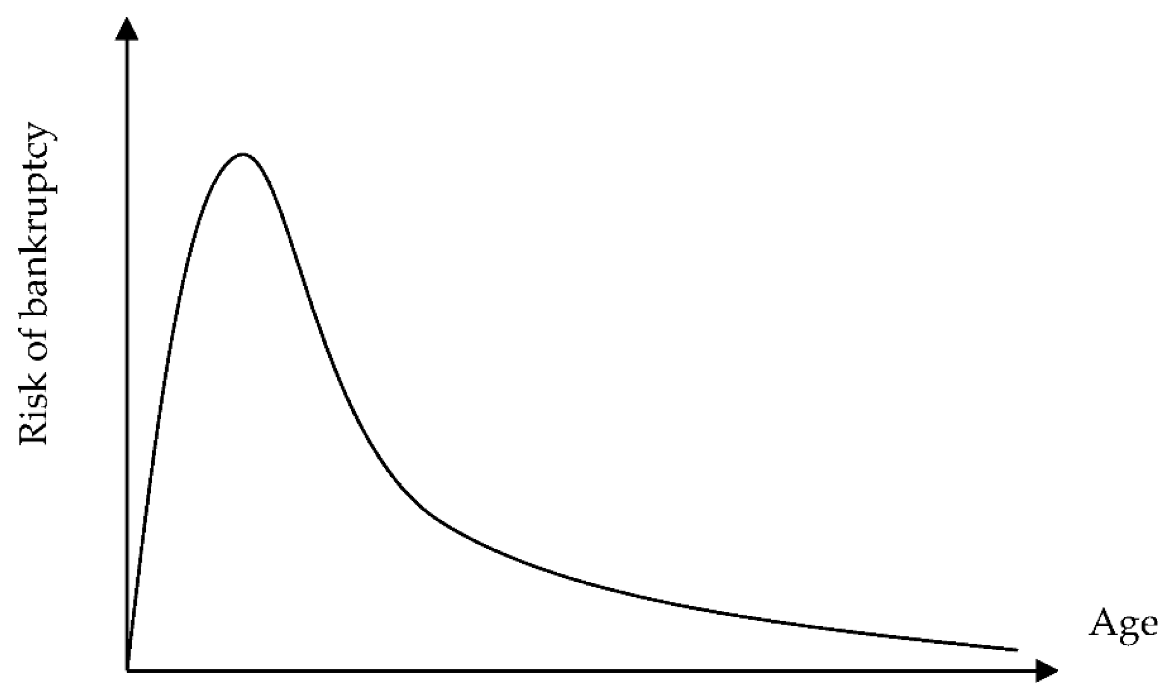
The last important topic to consider in developing bankruptcy forecasting models is the structure of enterprises in research sample regarding their age and type of industry they operate in. In the literature, studies of individual authors (e.g., Cressy 2006) confirm the assumptions of the theoretical model developed by Jovanovic (1982). He reveals the effect of company age on the risk of bankruptcy is in the form of an inverted U shape (Figure 2).
Jovanovic suggests that after entering the market, the company begins to learn to recognize its earning potential, competitiveness, and efficiency. Research by Pakes and Ericsson (1998) has shown that the company needs time to gain that knowledge and experience to manage crisis situations. The studies of Bradley and Rubach (2002) also showed that the second and third year of existence has the highest risk of bankruptcy (52% of cases). The studies of Doyle et al. (2007) confirm that the older the company, the more established its market position but also internal financial control.
The second demographic factor influencing the susceptibility of a company to risk of bankruptcy is the type of industry in which the company operates. According to the director of the international rating agency Standard & Poor’s, the type of industry affects the risk of deterioration in financial situation of companies by such factors as (Ganguin and Bilardello 2005):
  • Intensity of competition,
  • Life cycle of products,
  • The demand,
  • Changes in consumer preferences,
  • Technological change,
  • Reducing entry barriers into the industry,
  • Susceptibility of the industry to business cycle.
Ganguin and Bilardello (2005) emphasize that each industry has different risk parameters. In the 21st century, in an era of intense globalization, product life cycles in some industries are getting much shorter, often with increasing intensity of competition by reducing entry barriers into the industry. These authors rank industries into three risk levels:
  • Riskiest sectors—industry: Metal, mining, automotive, aerospace, housing, paper,
  • Medium risk industries—restaurants, retail, medical sector, tourism, transport,
  • Least risky sectors—journalistic, military, pharmaceutical industry, and agriculture.
Chava and Jarrow (2004) in their studies also have demonstrated the impact of the type of industry on the bankruptcy of enterprises. They divided the population of 1461 bankrupt American joint-stock companies into 10 types of industries. Using bankruptcy prediction models by Altman, Shumway, and Żmijewski, they proved that the type of industry affects the correct coefficients in each model.

3. Data, Samples, and Modeling Methods

To address all the issues in forecasting corporate bankruptcy risk described in the previous section, the author of the paper in developing learning and the testing sample:
  • Has chosen a clear definition of “bankrupt” enterprises. The enterprises at risk of bankruptcy were chosen based on the following three criteria: Information from the firm’s authorities about the risk of financial failure, court judgments declaring bankruptcy, and liquidation of the company;
  • Has chosen four prediction methods that do not allow manipulation of thresholds—multilayer neural network, recurrent neural network, fuzzy sets, and decision trees;
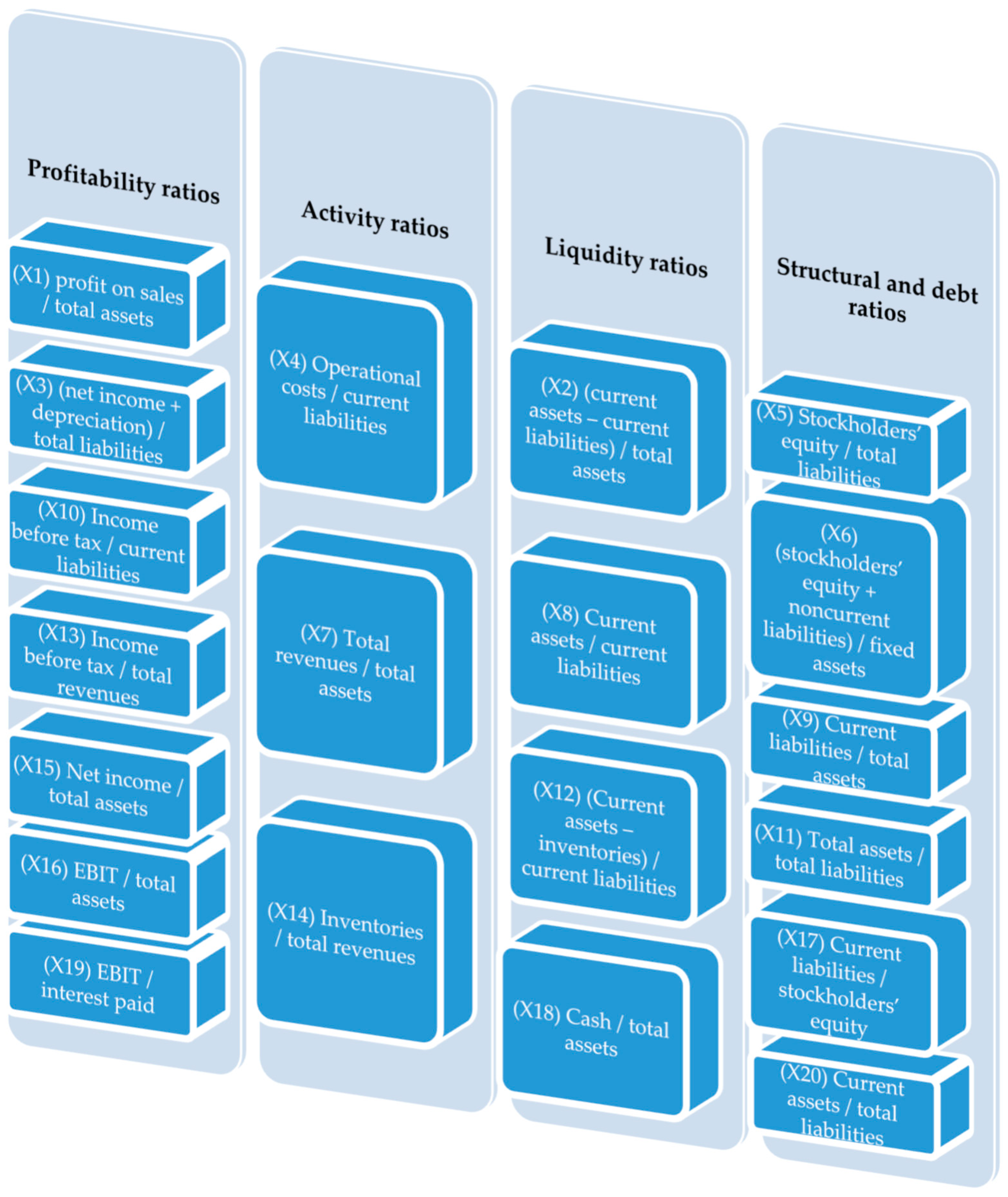
  • Has calculated 20 financial ratios (Figure 3) for all the enterprises (bankrupt and non-bankrupt) for whole analyzed period of 10 years prior to bankruptcy and the dynamics for all ratios. The assumption was to build the models with at least two variables representing the change of value of financial ratio to avoid stationarity of the created models;
  • Has selected enterprises that were operating in the market for at least 10 years (to avoid the selection of new, young companies characterized with higher bankruptcy risk).
The forecasting horizon for all enterprises and all models comprises 10 periods: From one year to 10 years prior to bankruptcy. Such a research approach allows the identification of which model characterizes the forecast with the smallest decrease of effectiveness along the increasing horizon and verifies the influence of implementing dynamic elements to the models on its effectiveness. Depending on the enterprise, the 10-year financial statements taken for analysis covered the period from 2004 to 2017.
The learning and testing samples comprise enterprises from European countries (Germany, France, UK, Spain, Finland, Italy, Poland, Sweden, Denmark). Each testing sample includes 250 bankrupt and 250 non-bankrupt enterprises, while each learning sample includes 50 bankrupt and 50 non-bankrupt firms. Both samples consist of companies that are publicly traded, due to better availability of financial data of firms in case of such a long-term forecasting horizon (10 years prior to bankruptcy). The research contains the firms of all sizes (small, medium, and large) keeping the principle of pairing the same size and sector of bankrupt firms to non-bankrupt ones.
To assess the effectiveness of the created models, three evaluation metrics were calculated for each testing sample: Overall effectiveness and Type I and Type II errors. Overall effectiveness is calculated based on how many enterprises are correctly classified by the forecasting model in a given testing sample:
S = {1 − [(D1 + D2)/(BR + NBR)]} ∗ 100%
where D1 is the number of bankrupt firms classified by the model as non-bankrupt, D2 is the number of non-bankrupt enterprises classified by the model as bankrupt, BR is the number of bankrupt companies in the sample, and NBR is the number of non-bankrupt companies in the sample.
Type I error is a measure of the number of firms in which the model incorrectly classifies a bankrupt firm into a non-bankrupt class, while Type II error is a measure that accounts for the number of firms classified as bankrupt when they actually belong to a non-bankrupt class.
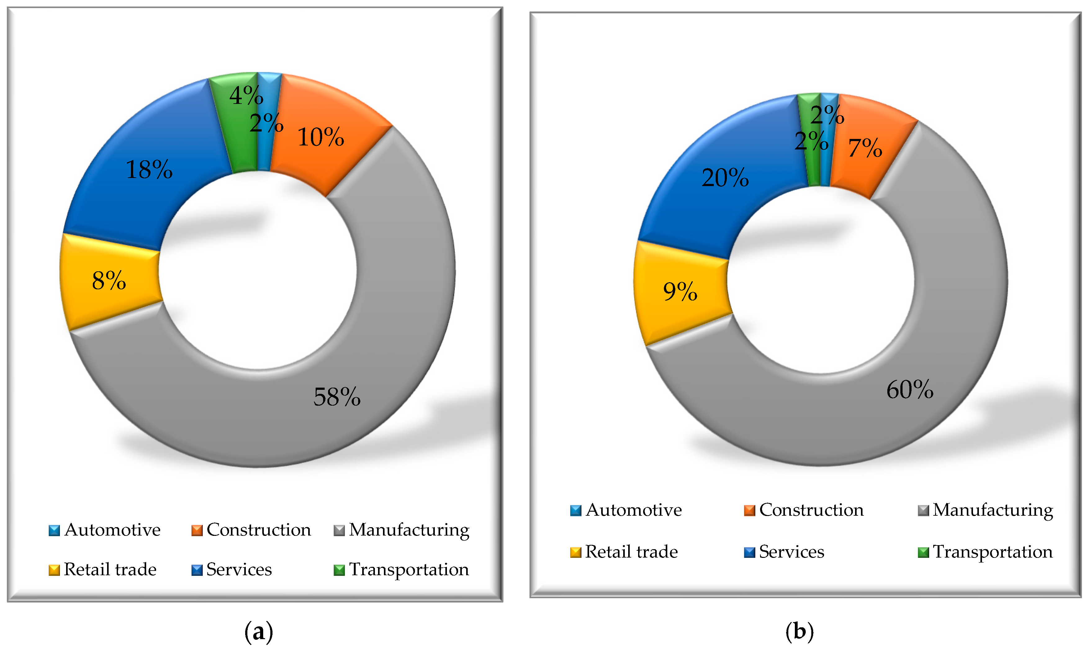
To ensure the reliable process of learning and testing the models, the enterprises were selected for both samples while maintaining very similar structure of belonging to sectors of industry. From Figure 4 it can be seen that the biggest number of enterprises was for manufacturing companies (58% and 60% of all firms in the learning and testing datasets, respectively). Although the automotive industry is part of manufacturing sector, it was distinguished separately from manufacturing industry as in many countries it has big influence on the whole economy, indirectly affecting also the financial situation of enterprises from other sectors. The second biggest share accounted for service companies—18% of all firms in learning and 20% of all firms in testing sample. Such a balanced number of sectors between the two samples should ensure the reliability of results.

4. Results and Discussion

In the first stage of research, the author developed two artificial neural network models—multilayer and recurrent. Inputs to the models were chosen based on the correlation matrix by choosing only the features that were poorly correlated with each other and strongly correlated with the grouping variable, representing the information about the risk of bankruptcy. This approach ensured the selection of such features, which do not duplicate information provided by other financial ratios, while being good representatives of the ratios not selected as diagnostic. The following financial ratios were set (the formulas are given in Figure 3): X1 (profitability ratio), X6 (structural ratio), X7 (activity ratio), X8 (liquidity ratio), DX1 (dynamics of ratio X1), DX8 (dynamics of ratio X8). It can be seen that each ratio belongs to a different field of financial analysis.
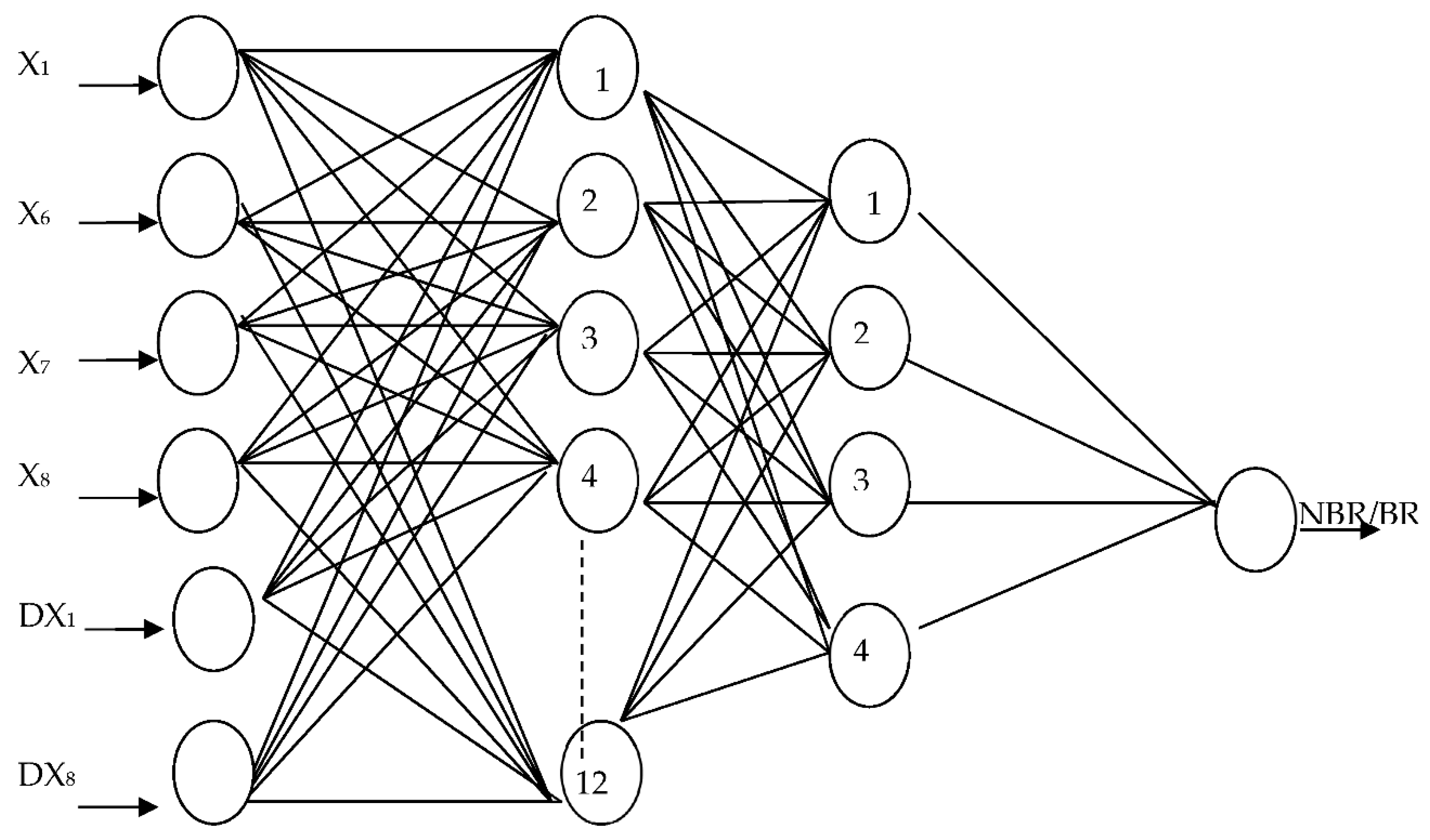
The multilayer neural network is the network in which the signal flow is only in one direction, from the input (financial ratios) through the hidden layer, where the main processing of neural signals takes place, to the output, where the network provides a forecast (bankrupt/non-bankrupt). The architecture of the developed multilayer network is shown in Figure 5. At the entry layer there are six neurons, in the first hidden layer there are 12 neurons (double the number of neurons as entry ones), in the second hidden layer there are four neurons and then one single output neuron where the forecast is generated.
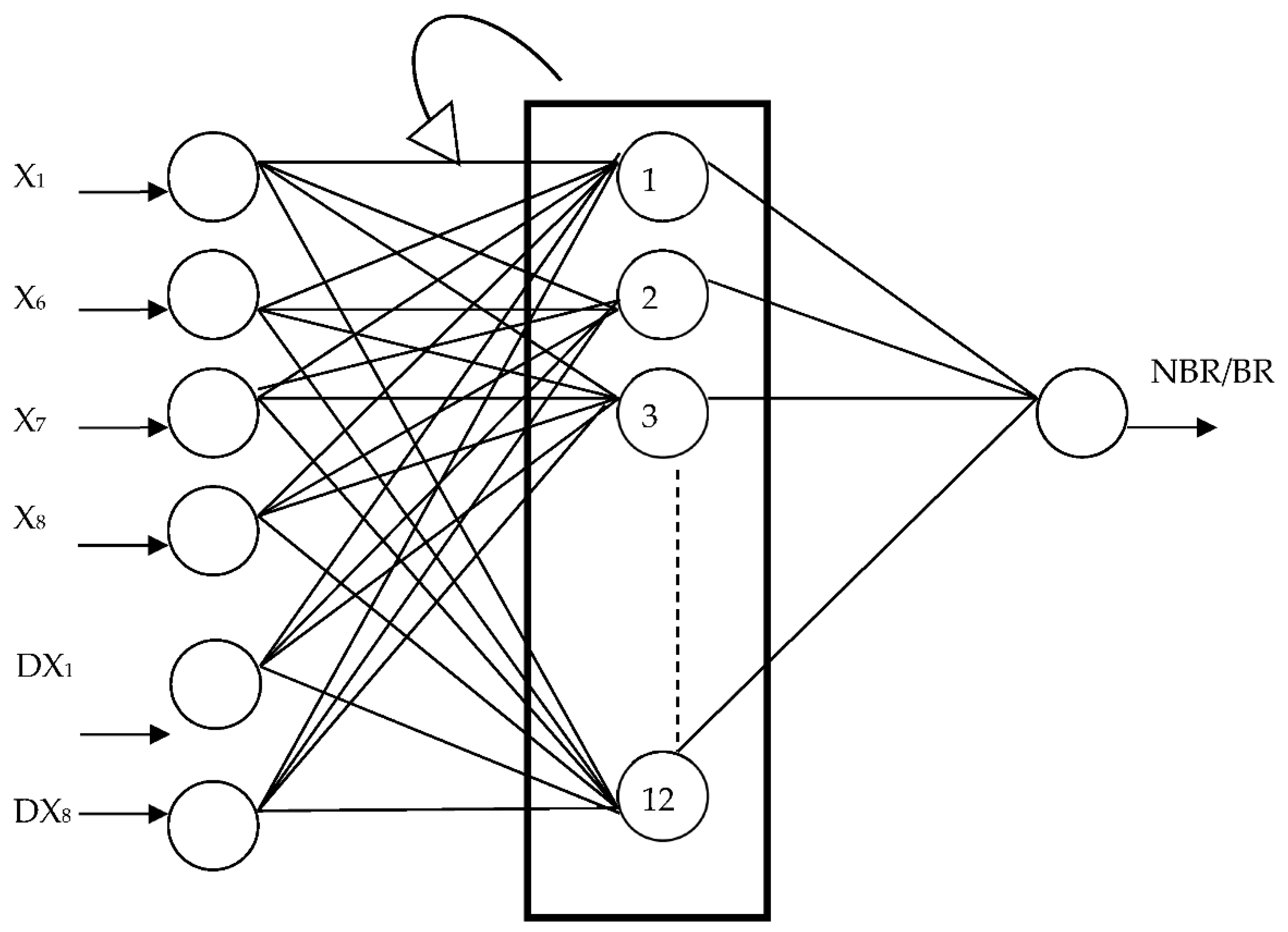
In topology of recurrent networks, it is acceptable to use reverse connections. The output from any neuron can be passed also to its input. Neuron state is therefore dependent not only on the value of the input signal (financial ratio), but also on the past state of any neuron, not excluding this particular neuron. The network response to specific input takes in this case an iterative character. The created architecture of the recurrent neural network for predicting risk of bankruptcy for European companies is shown in Figure 6. The developed recurrent model has the same entry layer as the previous model, but it consists of only one hidden layer with 12 neurons as the reverse connections between neurons support higher computing properties.
The next developed model was fuzzy sets model. This model requires no assumptions about the learning process and is developed based on expert knowledge and experience. The decision-making center of the fuzzy logic model is the base of rules in the form: IF-THEN, written by the author of this paper. The output of the model is a variable representing the forecast of the financial situation of the audited company. This variable has a value from 0 to 1, and it was assumed that the threshold dividing companies into at risk and not at risk of bankruptcy is 0.5. For each input, that is the financial ratio, the author defined critical value (Table 1). The fuzzy sets model consists the same entry variables as both created neural networks.
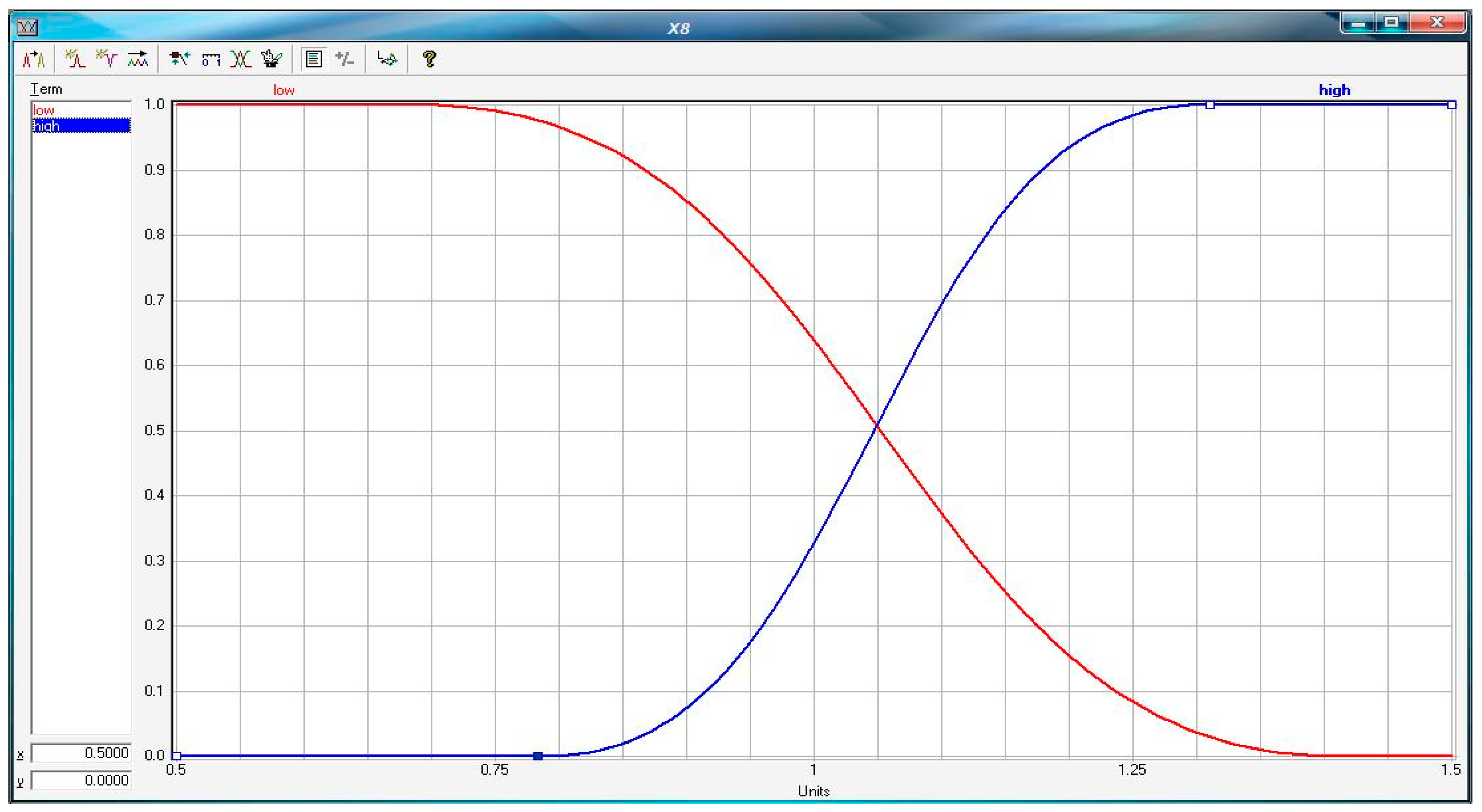
To explain more how the fuzzy sets model functions, below is an example of fuzzy sets defined using membership functions for the ratio X8 (Figure 7).
For ratio X8, shown in Figure 7 (this ratio represents current liquidity of firms), the threshold between a positive and negative situation is the value of 1.05. All values less than 0.7 are strictly negative, i.e., they belong to the fuzzy subset “LOW” with the degree of membership of 1 and to a subset “HIGH” with the degree of membership equal to 0. All values greater than 1.3 are strictly positive and, therefore, belong to the fuzzy subset “LOW” with the degree of membership of 0 and to the subset “HIGH” with the degree of membership equal to 1. Values contained in the range from 0.7 to 1.3 belong to both fuzzy subsets with different values of membership functions, e.g., for values of X8 equal to 1.05, the value of the function of membership in the “LOW” set is 0.5 and for the “HIGH” set is 0.5. With such defined subsets, the boundary between the values considered positive or negative is fuzzificated—a certain ratio value is “partially high” and “partially low”. There is no such possibility in the case of classical logic, which is bivalent and in which the value of the ratio is “high” or “low”. Therefore, the use of classical logic in assessing the financial situation of enterprises negatively affects the effectiveness of forecasts. This is true particularly for values close to the border of subsets, where a slight excess in the critical values of the ratio determines the final assessment (as completely positive or negative), which is not true because both values of the ratio reflect almost the same situation in the firm.
The author has developed the following 36 decision-making “IF-THEN” rules for the fuzzy sets model:
  • If X1 <= 0.015 and X6 <= 0.9 and X7 <= 0.82 and X8 <= 1.05 and DX1 <= 70 and DX8 <= 85 then 0
  • If X1 <= 0.015 and X6 <= 0.9 and X7 <= 0.82 and X8 <= 1.05 and DX1 > 70 and DX8 <= 85 then 0
  • If X1 <= 0.015 and X6 <= 0.9 and X7 <= 0.82 and X8 > 1.05 and DX1 > 70 and DX8 <= 85 then 0
  • If X1 <= 0.015 and X6 <= 0.9 and X7 > 0.82 and X8 > 1.05 and DX1 > 70 and DX8 <= 85 then 1
  • If X1 <= 0.015 and X6 > 0.9 and X7 > 0.82 and X8 > 1.05 and DX1 > 70 and DX8 <= 85 then 1
  • If X1 > 0.015 and X6 > 0.9 and X7 > 0.82 and X8 > 1.05 and DX1 > 70 and DX8 <= 85 then 1
  • If X1 <= 0.015 and X6 <= 0.9 and X7 > 0.82 and X8 <= 1.05 and DX1 > 70 and DX8 <= 85 then 0
  • If X1 <= 0.015 and X6 > 0.9 and X7 <= 0.82 and X8 <= 1.05 and DX1 > 70 and DX8 <= 85 then 0
  • If X1 > 0.015 and X6 <= 0.9 and X7 <= 0.82 and X8 <= 1.05 and DX1 > 70 and DX8 <= 85 then 0
  • If X1 <= 0.015 and X6 <= 0.9 and X7 <= 0.82 and X8 > 1.05 and DX1 <= 70 and DX8 <= 85 then 0
  • If X1 <= 0.015 and X6 <= 0.9 and X7 > 0.82 and X8 <= 1.05 and DX1 <= 70 and DX8 <= 85 then 0
  • If X1 <= 0.015 and X6 > 0.9 and X7 <= 0.82 and X8 <= 1.05 and DX1 <= 70 and DX8 <= 85 then 0
  • If X1 > 0.015 and X6 <= 0.9 and X7 <= 0.82 and X8 <= 1.05 and DX1 <= 70 and DX8 <= 85 then 0
  • If X1 <= 0.015 and X6 > 0.9 and X7 > 0.82 and X8 > 1.05 and DX1 <= 70 and DX8 <= 85 then 1
  • If X1 <= 0.015 and X6 <= 0.9 and X7 > 0.82 and X8 > 1.05 and DX1 <= 70 and DX8 <= 85 then 0
  • If X1 <= 0.015 and X6 > 0.9 and X7 <= 0.82 and X8 > 1.05 and DX1 <= 70 and DX8 <= 85 then 0
  • If X1 <= 0.015 and X6 > 0.9 and X7 > 0.82 and X8 <= 1.05 and DX1 <= 70 and DX8 <= 85 then 0
  • If X1 > 0.015 and X6 <= 0.9 and X7 > 0.82 and X8 <= 1.05 and DX1 <= 70 and DX8 <= 85 then 0
  • If X1 > 0.015 and X6 <= 0.9 and X7 <= 0.82 and X8 > 1.05 and DX1 <= 70 and DX8 <= 85 then 0
  • If X1 > 0.015 and X6 <= 0.9 and X7 <= 0.82 and X8 > 1.05 and DX1 > 70 and DX8 <= 85 then 1
  • If X1 > 0.015 and X6 > 0.9 and X7 <= 0.82 and X8 > 1.05 and DX1 > 70 and DX8 <= 85 then 1
  • If X1 > 0.015 and X6 > 0.9 and X7 <= 0.82 and X8 <= 1.05 and DX1 > 70 and DX8 <= 85 then 1
  • If X1 > 0.015 and X6 > 0.9 and X7 > 0.82 and X8 <= 1.05 and DX1 <= 70 and DX8 <= 85 then 1
  • If X1 > 0.015 and X6 > 0.9 and X7 <= 0.82 and X8 > 1.05 and DX1 <= 70 and DX8 <= 85 then 1
  • If X1 > 0.015 and X6 <= 0.9 and X7 > 0.82 and X8 > 1.05 and DX1 > 70 and DX8 <= 85 then 1
  • If X1 <= 0.015 and X6 <= 0.9 and X7 <= 0.82 and X8 <= 1.05 and DX1 <= 70 and DX8 > 85 then 0
  • If X1 <= 0.015 and X6 <= 0.9 and X7 <= 0.82 and X8 <= 1.05 and DX1 > 70 and DX8 > 85 then 0
  • If X1 <= 0.015 and X6 <= 0.9 and X7 <= 0.82 and X8 > 1.05 and DX1 > 70 and DX8 > 85 then 1
  • If X1 <= 0.015 and X6 <= 0.9 and X7 > 0.82 and X8 > 1.05 and DX1 > 70 and DX8 > 85 then 1
  • If X1 <= 0.015 and X6 > 0.9 and X7 > 0.82 and X8 > 1.05 and DX1 > 70 and DX8 > 85 then 1
  • If X1 > 0.015 and X6 > 0.9 and X7 > 0.82 and X8 > 1.05 and DX1 > 70 and DX8 > 85 then 1
  • If X1 > 0.015 and X6 <= 0.9 and X7 <= 0.82 and X8 <= 1.05 and DX1 <= 70 and DX8 > 85 then 0
  • If X1 > 0.015 and X6 > 0.9 and X7 <= 0.82 and X8 <= 1.05 and DX1 <= 70 and DX8 > 85 then 1
  • If X1 <= 0.015 and X6 <= 0.9 and X7 > 0.82 and X8 <= 1.05 and DX1 > 70 and DX8 > 85 then 1
  • If X1 <= 0.015 and X6 > 0.9 and X7 <= 0.82 and X8 > 1.05 and DX1 <= 70 and DX8 > 85 then 1
  • If X1 > 0.015 and X6 > 0.9 and X7 > 0.82 and X8 <= 1.05 and DX1 <= 70 and DX8 > 85 then 1
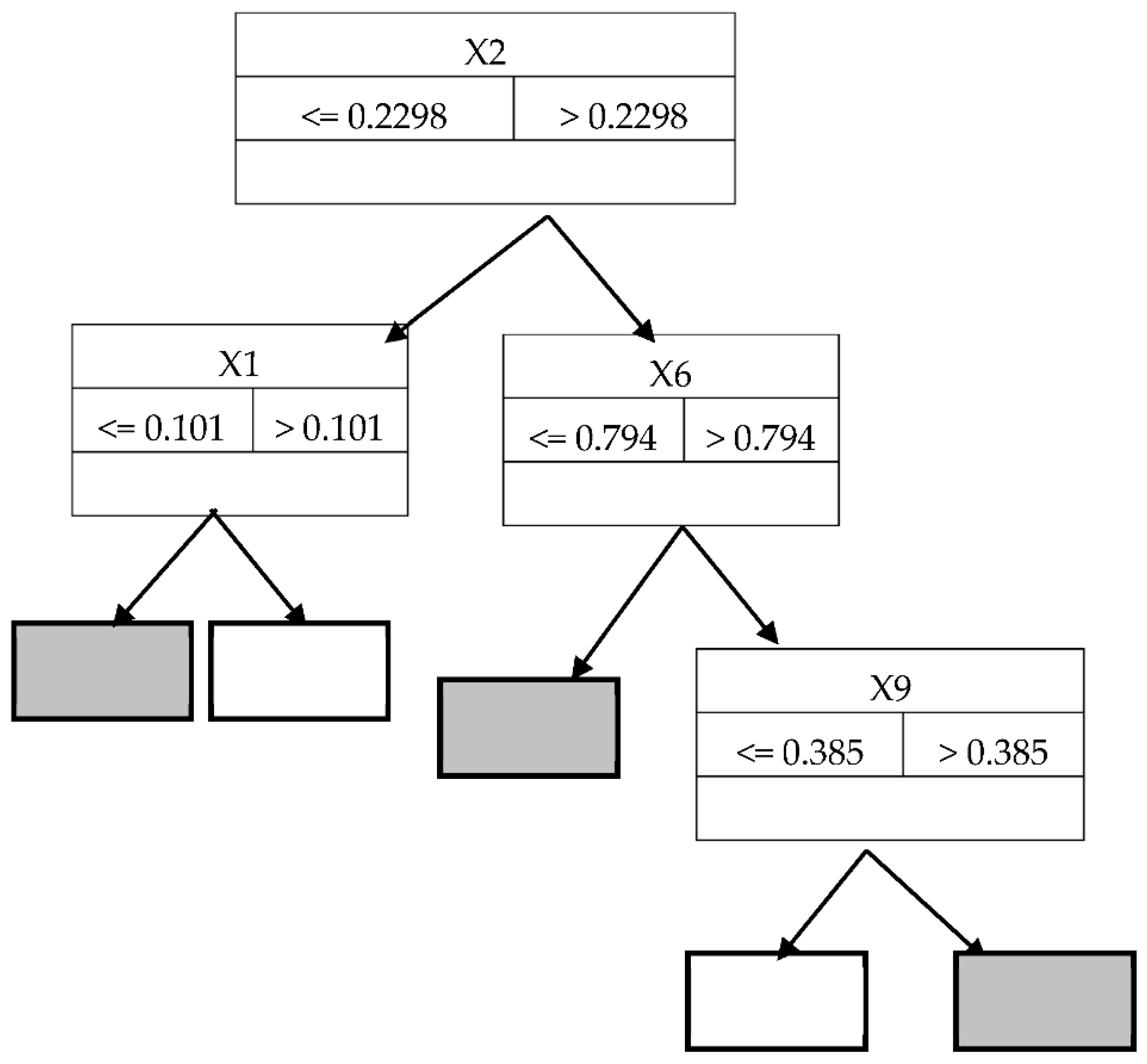
In the last stage of the research, the author estimated the decision trees model. The structure of the model is presented in Figure 8. In this model, the following financial ratios were selected: X2 (liquidity ratio), X1 (profitability ratio), X6 (structural ratio), X9 (structural ratio). As can be seen in this model, none of variables representing the change of value of ratios (dynamics) were selected during estimation process of the model. This means it is the only static model in the proposed research.
When evaluating the effectiveness of the developed models (Table 2), we can draw the following conclusions:
  • During the whole analyzed period (all 10 years prior to bankruptcy) the highest effectiveness was achieved using the fuzzy sets model, with 96.2% correct classifications one year before bankruptcy, 95.4% correct classifications two years prior to financial failure, and 93.8% correct classifications three years before bankruptcy;
  • The second best forecasting model is the recurrent neural network model with an effectiveness from 91.2% three years before financial crisis to up to 95.2% correct classifications one year prior to bankruptcy;
  • An examination of the effectiveness of the dynamic models (fuzzy sets, multilayer and recurrent neural networks) shows that all of them stand out with very good results in the forecasting horizon of up to six years prior to bankruptcy, with an effectiveness above 80%;
  • The effectiveness of the static decision tree model is smaller than the effectiveness of the dynamic models for all the analyzed years. Additionally, the model shows significantly bigger decrease of effectiveness while prolonging the period of the forecast than dynamic models;
  • The fuzzy sets model as the only dynamic model maintained an effectiveness level above 70% until the eighth year prior to bankruptcy;
  • Moreover, all three dynamic models have the fewest Type I errors. Such errors indicate how many bankrupt enterprises are classified as non-bankrupt firms. Type I errors, for obvious financial reasons, are far more dangerous than Type II errors.

5. Conclusions

This paper presents how to improve the effectiveness of forecasting corporate distress risk models in both the short and long horizon, exceeding five years before the announcement of bankruptcy.
The present empirical study reveals that the implementation of dynamic elements to the forecasting models positively affects the effectiveness and the stability of the forecast. The dynamic models generate a smaller number of errors, and the decrease of effectiveness of such models is smaller with extending the forecast period than in the case of static models. Additionally, this research also proved the superiority of fuzzy sets model over the other developed models, both in terms of effectiveness during all analyzed years prior to bankruptcy and in terms of the smallest decrease of predictive abilities while increasing the forecasting horizon.
The main limitation of the research is limited financial data access, especially for bankrupt enterprises (in many cases there are data available only for one to three years before the enterprise went bankrupt, which makes it difficult to conduct the research in such long horizon of 10 years prior to financial failure). That is why the studies are focused on countries with better organized financial reporting systems (EU countries). The author is going to continue the research towards the use of macroeconomic variables of selected countries in predicting the risk of bankruptcy of enterprises.

Funding

This research has been prepared within the grant project No. 2015/19/B/HS4/00377, “Trajectories of life and the collapse of companies in Poland and in the world—identification, evaluation and forecast”. Research funded by the National Science Centre in Poland (Narodowe Centrum Nauki).

Conflicts of Interest

The author declares no conflict of interest. The funders had no role in the design of the study; in the collection, analyses, or interpretation of data; in the writing of the manuscript, or in the decision to publish the results.

References

  1. Acosta-González, Eduardo, and Fernando Fernández-Rodríguez. 2014. Forecasting financial failure of firms via genetic algorithms. Computational Economics 43: 133–57. [Google Scholar] [CrossRef] [Green Version]
  2. Agarwal, Vineet, and Richard Taffler. 2007. Twenty-five years of the Taffler z-score model—Does it really have predictive ability? Accounting and Business Research 37: 285–300. [Google Scholar] [CrossRef]
  3. Ahn, Byeong, Sung Cho, and Chang Kim. 2000. The integrated methodology of rough set theory and artificial neural networks for business failure prediction. Expert Systems with Applications 18: 65–74. [Google Scholar] [CrossRef]
  4. Alaka, Hafiz A., Lukumon O. Oyedele, Hakeem A. Owolabi, Vikas Kumar, Saheed O. Ajayi, Olugbenga O. Akinade, and Muhammad Bilal. 2018. Systematic review of bankruptcy prediction models: Towards a framework for tool selection. Expert Systems with Applications 94: 164–84. [Google Scholar] [CrossRef]
  5. Altman, Edward. 1968. Financial ratios, discriminant analysis and the prediction of corporate bankruptcy. Journal of Finance 23: 589–609. [Google Scholar] [CrossRef]
  6. Altman, Edward. 2018. Applications of distress prediction models: What have we learned after 50 years from the Z-score models? International Journal of Financial Studies 6: 70. [Google Scholar] [CrossRef] [Green Version]
  7. Altman, Edward, and Herbert Rijken. 2006. A point-in-time perspective on through-the-cycle ratings. Financial Analysts Journal 62: 54–70. [Google Scholar] [CrossRef]
  8. Andres, Javier, Manuel Landajo, and Pedro Lorca. 2005. Forecasting business profitability by using classification techniques: A comparative analysis based on a Spanish case. European Journal of Operational Research 167: 518–42. [Google Scholar] [CrossRef]
  9. Atiya, Amir. 2001. Bankruptcy prediction for credit risk using neural networks: A survey and new results. IEEE Transactions on Neural Networks 12: 929–35. [Google Scholar] [CrossRef] [Green Version]
  10. Balcaen, Sofie, and Hubert Ooghe. 2006. 35 years of studies on business failure: An overview of the classic statistical methodologies and their related problems. The British Accounting Review 38: 63–93. [Google Scholar] [CrossRef]
  11. Bandyopadhyay, Arindam. 2006. Predicting probability of default of Indian corporate bonds: Logistic and Z-score model approaches. The Journal of Risk Finance 7: 255–72. [Google Scholar] [CrossRef]
  12. Barboza, Flavio, Herbert Kimura, and Edward Altman. 2017. Machine learning models and bankruptcy prediction. Expert Systems with Applications 83: 405–17. [Google Scholar] [CrossRef]
  13. Beaver, William H. 1966. Financial ratios as predictors of failure. Journal of Accounting Research 4: 71–111. [Google Scholar] [CrossRef]
  14. Berryman, John. 1992. Small Business Bankruptcy and Failure—A Survey of the Literature. Los Angeles: Small Business Research Institute of Industrial Economics, pp. 1–18. [Google Scholar]
  15. Brabazon, Anthony, and Michael O’Neil. 2004. Diagnosing corporate stability using grammatical evolution. Journal of Applied Mathematics and Computer Science 1: 293–310. [Google Scholar]
  16. Bradley, Don, and Michael Rubach. 2002. Trade Credit and Small Business—A Cause of Business Failures? Conway: University of Central Arkansas, pp. 1–7. [Google Scholar]
  17. Callejon, A.M., A.M. Casado, Martina Fernandez, and J.I. Pelaez. 2013. A system of insolvency prediction for industrial companies using a financial alternative model with neural networks. International Journal of Computational Intelligence Systems 6: 29–37. [Google Scholar] [CrossRef] [Green Version]
  18. Chava, Sudheer, and Robert Jarrow. 2004. Bankruptcy prediction with industry effects. Review of Finance 8: 537–69. [Google Scholar] [CrossRef]
  19. Cressy, Robert. 2006. Why do most firms die young? Small Business Economics 26: 103–16. [Google Scholar] [CrossRef]
  20. Crone, Sven, and Steven Finlay. 2012. Instance sampling in credit scoring: An empirical study of sample size and balancing. International Journal of Forecasting 28: 224–38. [Google Scholar] [CrossRef]
  21. Davies, David. 1997. The Art of Managing Finance. Lincoln: McGraw-Hill Book Co. [Google Scholar]
  22. Deakin, Edward B. 1972. A discriminant analysis of prediction of business failure. Journal of Accounting Research 3: 167–69. [Google Scholar] [CrossRef]
  23. Delen, Dursun, Cemil Kuzey, and Ali Uyar. 2013. Measuring firm performance using financial ratios: A decision tree approach. Expert Systems with Applications 40: 3970–83. [Google Scholar] [CrossRef]
  24. Dong, Manh Cuong, Shaonan Tian, and Cathy W.S. Chen. 2018. Predicting failure risk using financial ratios: Quantile hazard model approach. North American Journal of Economics and Finance 44: 204–20. [Google Scholar] [CrossRef]
  25. Doumpos, Michalis, and Constantin Zopounidis. 1999. A multinational discrimination method for the prediction of financial distress: the case of Greece. Multinational Finance Journal 3: 71–101. [Google Scholar] [CrossRef]
  26. Doyle, Jeffrey, Weili Geb, and Sarah McVay. 2007. Determinants of weaknesses in internal control over financial reporting. Journal of Accounting and Economics 44: 193–223. [Google Scholar] [CrossRef]
  27. Foster, George. 1986. Financial Statement Analysis, 2nd ed. New York: Prentice Hall. [Google Scholar]
  28. Ganguin, Blaise, and John Bilardello. 2005. Fundamentals of Corporate Credit Analysis, Standard & Poor’s. New York: McGraw-Hill. [Google Scholar]
  29. Garcia, Vincente, Ana I. Marques, J. Salvador Sanchez, and Humberto Ochoa-Dominguez. 2019. Dissimilarity-Based Linear Models for Corporate Bankruptcy Prediction. Computional Economics 53: 1019–31. [Google Scholar] [CrossRef]
  30. Giannopoulos, George, and Sindre Sigbjornsen. 2019. Prediction of bankruptcy using financial ratios in the Greek market. Theoretical Economics Letters 9: 1114–28. [Google Scholar] [CrossRef] [Green Version]
  31. Grice, John, and Michael Dugan. 2001. The limitations of bankruptcy prediction models—Some cautions for the researcher. Review of Quantitative Finance and Accounting 17: 151–66. [Google Scholar] [CrossRef]
  32. Ho, Chun-Yu, Patrick McCarthy, Yi Yang, and Xuan Ye. 2013. Bankruptcy in the pulp and paper industry: Market’s reaction and prediction. Empirical Economics 45: 1205–32. [Google Scholar] [CrossRef]
  33. Hosaka, Tadaaki. 2019. Bankruptcy prediction using imaged financial ratios and convolutional neural networks. Expert Systems with Applications 117: 287–99. [Google Scholar] [CrossRef]
  34. Hosmer, David, Stanley Lemeshow, and Rod X. Sturdivant. 2013. Applied Logistic Regression. Hoboken: John Wiley & Sons. [Google Scholar]
  35. Jackson, Richard H.G., and Anthony Wood. 2013. The performance of insolvency prediction and credit risk models in the UK: A comparative study. The British Accounting Review 45: 183–202. [Google Scholar] [CrossRef]
  36. Jardin, Philippe. 2015. Bankruptcy prediction using terminal failure processes. European Journal of Operational Research 242: 286–303. [Google Scholar] [CrossRef]
  37. Jardin, Philippe. 2016. A two-stage classification technique for bankruptcy prediction. European Journal of Operational Research 254: 236–52. [Google Scholar] [CrossRef]
  38. Jardin, Philippe. 2017. Dynamics of firm financial evolution and bankruptcy prediction. Expert Systems with Applications 75: 25–43. [Google Scholar] [CrossRef]
  39. Jardin, Philippe. 2018. Failure pattern-based ensembles applied to bankruptcy forecasting. Decision Support Systems 107: 64–77. [Google Scholar] [CrossRef]
  40. Jardin, Philippe, and Eric Severin. 2011. Predicting corporate bankruptcy using a self-organizing map—An empirical study to improve the forecasting horizon of a financial failure model. Decision Support Systems 51: 701–11. [Google Scholar] [CrossRef] [Green Version]
  41. Jayasekera, Ranadeva. 2018. Prediction of company failure: Past, present and promising directions for the future. International Review of Financial Analysis 55: 196–208. [Google Scholar] [CrossRef]
  42. Jovanovic, Boyan. 1982. Selection and the evolution of industry. Econometrica 50: 649–70. [Google Scholar] [CrossRef]
  43. Kieschnick, Robert, Mark La Plante, and Rabih Moussawi. 2013. Working capital management and shareholders’ wealth. Review of Finance 17: 1827–52. [Google Scholar] [CrossRef]
  44. Kim, Myoung-Jong, and Dae-Ki Kang. 2010. Ensemble with neural networks for bankruptcy prediction. Expert Systems with Applications 37: 3373–79. [Google Scholar] [CrossRef]
  45. Kumar, Pramod, and Vadlamani Ravi. 2007. Bankruptcy prediction in banks and firms via statistical and intelligent techniques—A review. European Journal of Operational Research 180: 1–28. [Google Scholar] [CrossRef]
  46. Laitinen, Erkki K. 2007. Classification accuracy and correlation—LDA in failure prediction. European Journal of Operational Research 183: 210–25. [Google Scholar] [CrossRef]
  47. Lensberg, Terje, Aasmund Eilifsen, and Thomas E. McKee. 2006. Bankruptcy theory development and classification via genetic programming. European Journal of Operational Research 169: 677–97. [Google Scholar] [CrossRef]
  48. Li, Leon, and Robert Faff. 2019. Predicting corporate bankruptcy: What matters? International Review of Economics & Finance 62: 1–19. [Google Scholar]
  49. Liang, Deron, Chia-Chi Lu, Chih-Fong Tsai, and Guan-An Shih. 2016. Financial ratios and corporate governance indicators in bankruptcy prediction: A comprehensive study. European Journal of Operational Research 252: 561–72. [Google Scholar] [CrossRef]
  50. Lin, Fengyi, Deron Liang, Ching-Chiang Yeh, and Jui-Chieh Huang. 2014. Novel feature selection methods to financial distress prediction. Expert Systems with Applications 41: 2472–83. [Google Scholar] [CrossRef]
  51. Lukason, Oliver, and Richard C. Hoffman. 2014. Firm Bankruptcy Probability and Causes: An Integrated Study. International Journal of Business and Management 9: 80–91. [Google Scholar] [CrossRef] [Green Version]
  52. Lyandres, Evgeny, and Alexei Zhdanov. 2013. Investment opportunities and bankruptcy prediction. Journal of Financial Markets 16: 439–76. [Google Scholar] [CrossRef]
  53. Mcleay, Stuart, and Azmi Omar. 2000. The sensitivity of prediction models to the non-normality of bounded and unbounded financial ratios. British Accounting Review 32: 213–30. [Google Scholar] [CrossRef]
  54. Mensah, Yaw. 1984. An examination of the stationarity of multivariate bankruptcy prediction models—A methodological study. Journal of Accounting Research 22: 380–95. [Google Scholar] [CrossRef]
  55. Mihalovic, Matus. 2016. Performance Comparison of Multiple Discriminant Analysis and Logit Models in Bankruptcy Prediction. Economics and Sociology 9: 101–18. [Google Scholar] [CrossRef]
  56. Min, Jae, and Young-Chan Lee. 2005. Bankruptcy prediction using support vector machine with optimal choice of kernel function parameters. Expert Systems with Applications 28: 603–14. [Google Scholar] [CrossRef]
  57. Nwogugu, Michael. 2007. Decision-making, risk and corporate governance—A critque of methodological issues in bankruptcy/recovery prediction models. Applied Mathematics and Computation 185: 178–96. [Google Scholar] [CrossRef]
  58. Orsenigo, Carlotta, and Carlo Vercellis. 2013. Linear versus nonlinear dimensionality reduction for banks credit rating prediction. Knowledge-Based Systems 47: 14–22. [Google Scholar] [CrossRef]
  59. Pakes, Ariel, and Richard Ericsson. 1998. Empirical implications of alternative models of firm dynamics. Journal of Economic Theory 79: 1–45. [Google Scholar] [CrossRef] [Green Version]
  60. Psillaki, Maria, Ioannis E. Tsolas, and Dimmitris Margaritis. 2010. Evaluation of credit risk based on firm performance. European Journal of Operational Research 201: 873–81. [Google Scholar] [CrossRef]
  61. Ptak-Chmielewska, Aneta. 2019. Predicting Micro-Enterprise Failures Using Data Mining Techniques. Journal of Risk and Financial Managament 12: 30. [Google Scholar] [CrossRef] [Green Version]
  62. Ravisankar, Pediredla, and Vadlamani Ravi. 2010. Financial distress prediction in banks using group method of data handling neural network, counter propagation neural network and fuzzy ARTMAP. Knowledge-Based Systems 23: 823–31. [Google Scholar] [CrossRef]
  63. Succurro, Marianna, Giuseppe Arcuri, and Giuseppina D. Constanzo. 2019. A combined approach based on robust PCA to improve bankruptcy forecasting. Review of Accounting and Finance 18: 296–320. [Google Scholar] [CrossRef]
  64. Sun, Jie, Hui Li, Qing-Hua Huang, and Kai-Yu He. 2014. Predicting financial distress and corporate failure—A review from the state-of-the-art definitions, modeling, sampling, and featuring approaches. Knowledge-Based Systems 57: 41–56. [Google Scholar] [CrossRef]
  65. Tam, Kar Yan. 1991. Neural network models and the prediction of bank bankruptcy. Omega 19: 429–45. [Google Scholar] [CrossRef]
  66. Tian, Shaonan, and Yan Yu. 2017. Financial ratios and bankruptcy predictions: An international evidence. International Review of Economics and Finance 51: 510–26. [Google Scholar] [CrossRef]
  67. Tian, Shaonan, Yan Yu, and Hui Guo. 2015. Variable selection and corporate bankruptcy forecasts. Journal of Banking & Finance 52: 89–100. [Google Scholar]
  68. Tsai, Chih-Fong. 2014. Combining cluster analysis with classifier ensembles to predict financial distress. Information Fusion 16: 46–58. [Google Scholar] [CrossRef]
  69. Watson, John, and Jim Everett. 1999. Small business failure rates-choice of definition and industry effects. International Small Business Journal 17: 33–49. [Google Scholar] [CrossRef]
  70. Wu, Desheng Dash, Yidong Zhang, Dexiang Wu, and David L. Olson. 2010. Fuzzy multi-objective programming for supplier selection and risk modeling: A possibility approach. European Journal of Operational Research 200: 774–87. [Google Scholar] [CrossRef]
  71. Xiao, Zhi, Xianglei Yang, Ying Pang, and Xin Dang. 2012. The prediction for listed companies’ financial distress by using multiple prediction methods with rough set and Dempster-Shafer evidence theory. Knowledge-Based Systems 26: 196–206. [Google Scholar] [CrossRef]
  72. Zapranis, Achilleas, and Demetrios Ginoglou. 2000. Forecasting corporate failure with neural network approach: The Greek case. Journal of Financial Management & Analysis 13: 11–21. [Google Scholar]
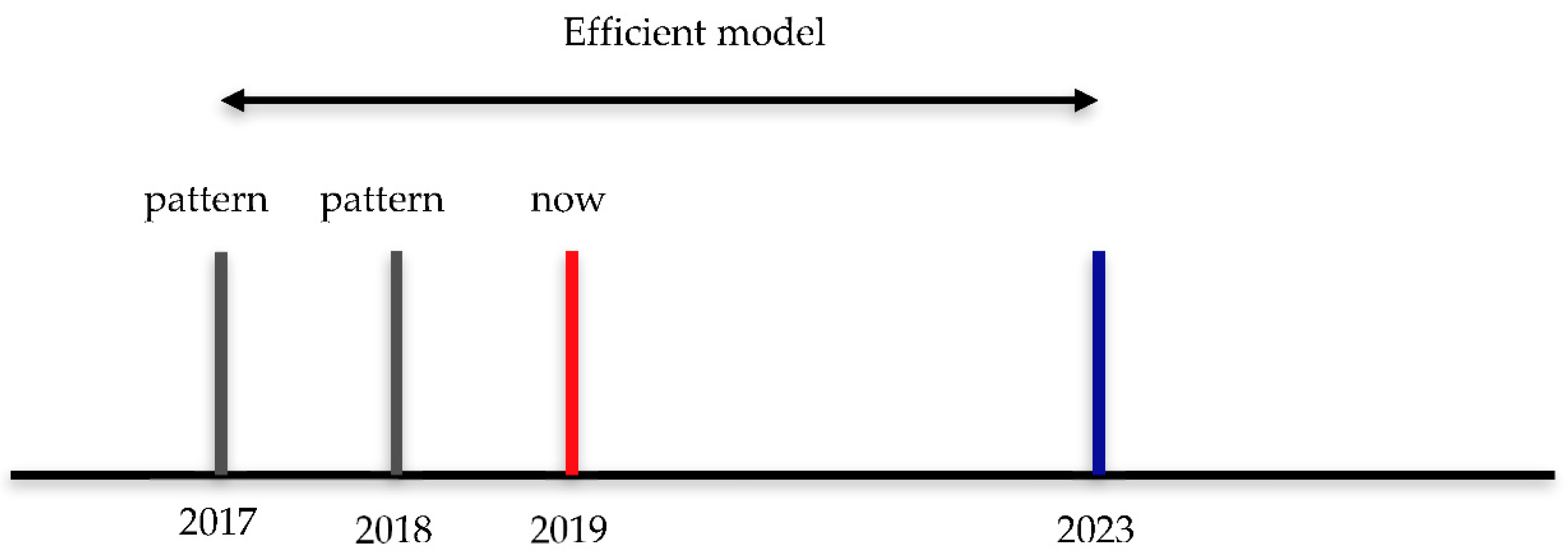
Figure 1. The life cycle of bankruptcy forecasting model. Source: Based on own studies.
Jrfm 12 00185 g001
Figure 2. Age of company and the risk of bankruptcy. Source: Based on own studies.
Jrfm 12 00185 g002
Figure 3. The financial ratios used in the study. Source: Self-study.
Jrfm 12 00185 g003
Figure 4. The sector structure of: (a) learning sample and (b) testing sample of enterprises. Source: Based on own studies.
Jrfm 12 00185 g004
Figure 5. Architecture of artificial feedforward multilayer neural network for analysis of enterprises. Source: Based on own studies.
Jrfm 12 00185 g005
Figure 6. Architecture of artificial recurrent neural network for analysis of enterprises. Source: Based on own studies.
Jrfm 12 00185 g006
Figure 7. Fuzzy sets for ratio X8 with membership functions. Source: Own studies conducted in MATLAB.
Jrfm 12 00185 g007
Figure 8. The structure of the Classification and Regression Tree (C&RT) model. Gray box indicates firms at risk of bankruptcy; white box, non-bankrupt firms. Source: based on own studies.
Jrfm 12 00185 g008
Table 1. Critical values of financial ratios used in the fuzzy sets model. Source: Based on own studies.
Indicator SymbolCritical Value in Fuzzy Sets Model
X10.015
X60.9
X70.82
X81.05
DX170.0%
DX885.0%
Table 2. The results of the effectiveness of models for European firms (testing sample). Source: Based on own studies.
Years Prior to BankruptcyMultilayer Neural NetworkRecurrent Neural NetworkFuzzy SetsDecision Trees
SE1E2SE1E2SE1E2SE1E2
1 year93.4%6.0%7.2%95.2%4.0%5.6%96.2%3.2%4.4%93.0%8.0%6.0%
2 years91.8%7.6%8.8%93.6%5.6%7.2%95.4%4.4%4.8%91.2%10.0%7.6%
3 years87.4%11.6%13.6%91.2%7.6%10.0%93.8%5.2%7.2%86.8%14.8%11.6%
4 years82.8%16.4%18.0%87.8%10.4%14.0%90.6%7.6%11.2%81.6%19.6%17.2%
5 years82.4%16.8%18.4%82.4%16.8%18.4%87.8%10.8%13.6%77.2%24.0%21.6%
6 years80.8%18.0%20.4%81.0%18.4%19.6%82.8%16.4%18.0%72.0%30.0%26.0%
7 years74.2%25.6%26.0%77.4%21.6%23.6%80.8%18.8%19.6%65.0%35.6%34.4%
8 years64.4%34.4%36.8%65.0%34.4%35.6%71.4%26.0%31.2%62.8%38.0%36.4%
9 years63.4%36.0%37.2%64.0%35.2%36.8%67.2%32.4%33.2%62.4%38.4%36.8%
10 years63.0%36.4%37.6%63.6%35.6%37.2%65.8%32.8%35.6%61.4%39.6%37.6%