How Long Does It Last to Systematically Make Bad Decisions? An Agent-Based Application for Dividend Policy


Abstract
1. Introduction
2. Theoretical Background
3. The Model
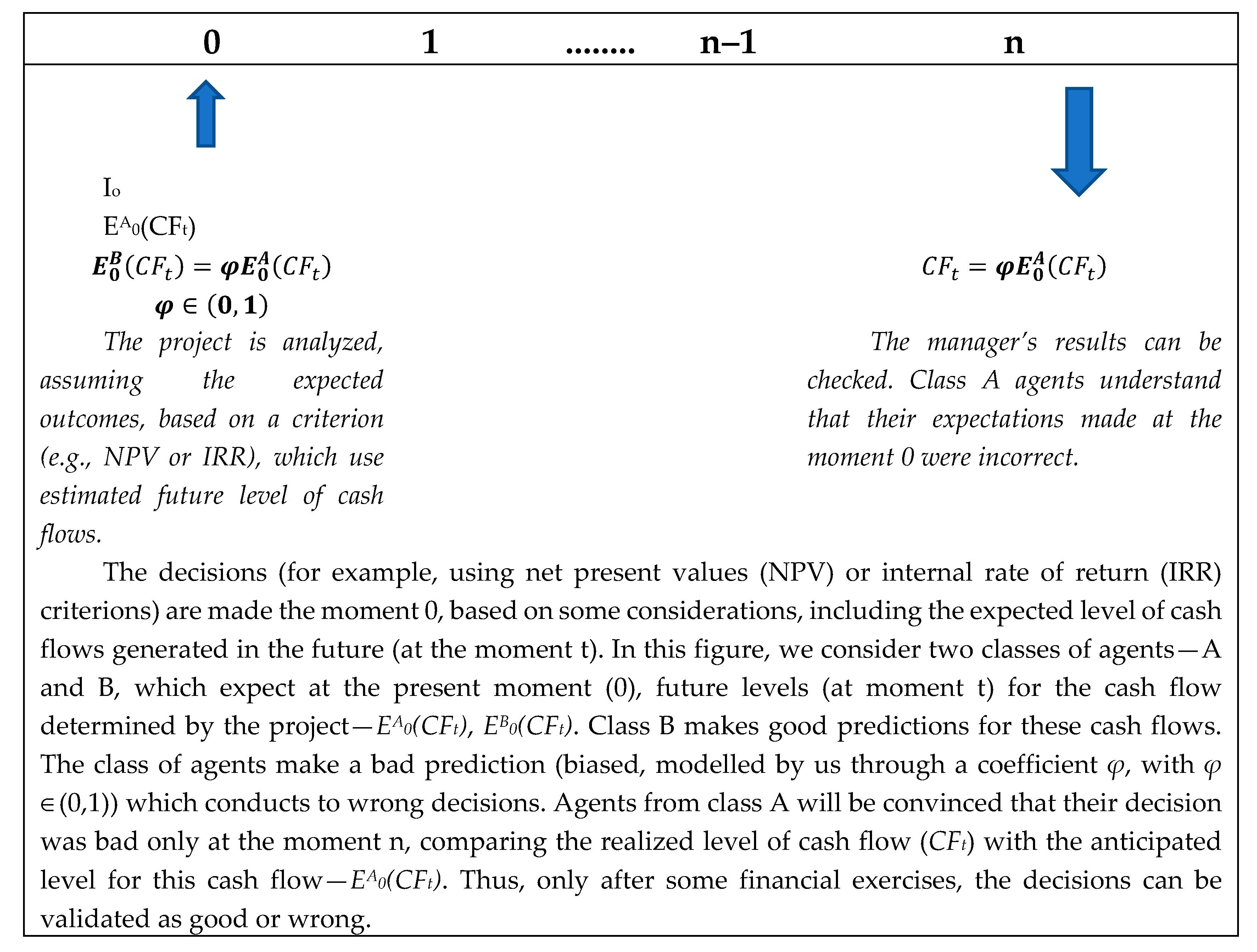
3.1. The Problem
3.2. Shareholders’ Typology and Behavior
3.3. Evolution of Return on Equity
3.4. Required Rates of Return
3.5. Model Inputs
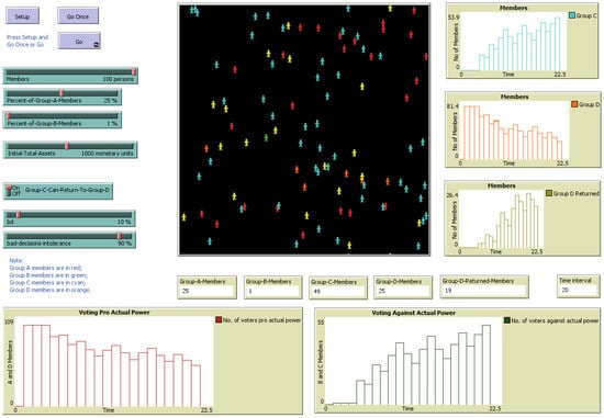
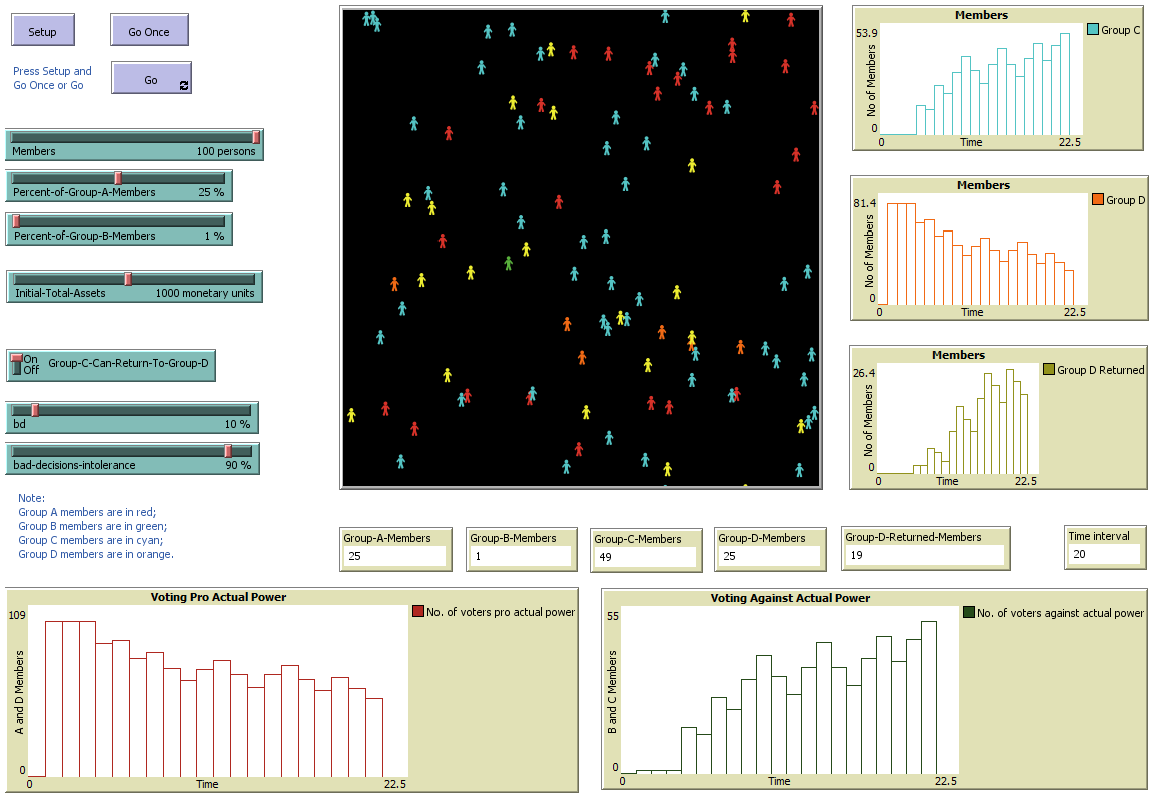
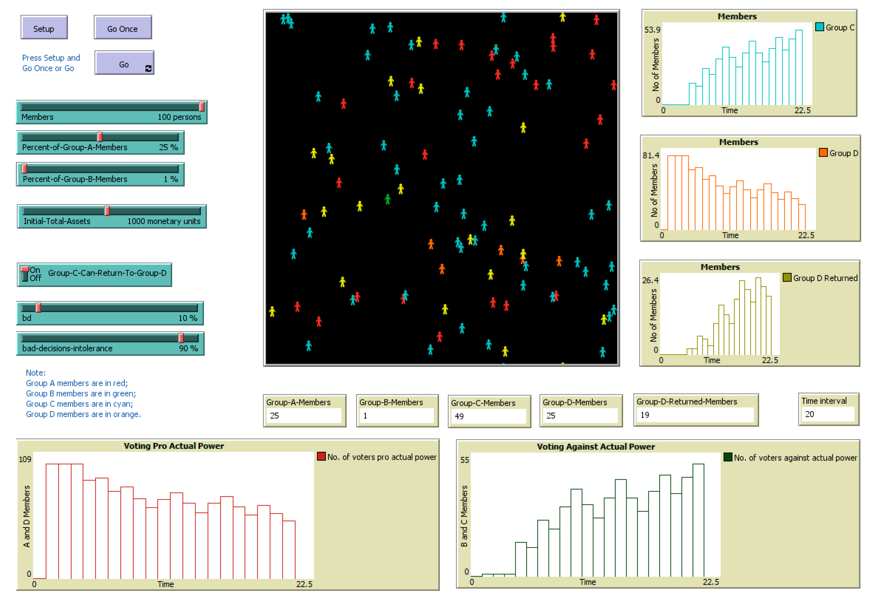
3.6. Implementation in NetLogo
4. Numerical Results: Discussion
5. Conclusions
Author Contributions
Funding
Acknowledgments
Conflicts of Interest
Appendix A. The NetLogo Code
References
- Aivazian, Varouj A., Laurence Booth, and Sean Cleary. 2006. Dividend Smoothing and Debt Ratings. Journal Financial and Quantitative Analysis 41: 439–53. [Google Scholar] [CrossRef]
- Ariely, Dan. 2009. The End of Rational Economics. Harvard Business Review 87: 78–84. [Google Scholar]
- Armeanu, Daniel Ştefan, Georgeta Vintilă, and Ștefan Cristian Gherghina. 2018. Empirical Study towards the Drivers of Sustainable Economic Growth in EU-28 Countries. Sustainability 10: 4. [Google Scholar] [CrossRef]
- Ballestero, Enrique, Mila Bravo, Blanca Perez-Gladish, Mar Arenas-Parra, and David Pla-Santamaria. 2012. Socially Responsible Investment: A multicriteria approach to portfolio selection combining ethical and financial objectives. European Journal of Operational Resrearch 216: 487–94. [Google Scholar] [CrossRef]
- Belghitar, Yacine, Ephraim Clark, and Konstantino Kassimatis. 2019. A measure of total firm performance: New insights for the corporate objective. Annals of Operations Research 281: 121–41. [Google Scholar] [CrossRef]
- Bhattacharya, Sudipto. 1979. Imperfect Information, Dividend Policy, and “The Bird in the Hand” Fallacy. Bell Journal of Economics 10: 259–70. [Google Scholar] [CrossRef]
- Bunn, Derek W., and Fernando S. Oliveira. 2003. Evaluating Individual Market Power in Electricity Markets via Agent-Based Simulation. Annals of Operations Research 121: 57–77. [Google Scholar] [CrossRef]
- Campbell, Andrew, Jo Whitehead, and Sydney Finkelstein. 2009. Why Good Leaders Make Bad Decisions. Harvard Business Review 87: 60–66. [Google Scholar]
- De Bondt, Werner F. M., and Richard H. Thaler. 1995. Chapter 13 Financial decision-making in markets and firms: A behavioral perspective. In Handbooks in Operations Research and Management Science. Edited by Robert Alan Jarrow, Vojislav Maksimovic and William T. Ziemba. Amsterdam: Elsevier, pp. 385–410. [Google Scholar] [CrossRef]
- Delcea, Camelia, Liviu-Adrian Cotfas, Nora Chiriță, and Ionuț Nica. 2018a. A Two-Door Airplane Boarding Approach When Using Apron Buses. Sustainability 10: 3619. [Google Scholar] [CrossRef]
- Delcea, Camelia, Liviu-Adrian Cotfas, and Ramona Păun. 2018b. Agent-Based Evaluation of the Airplane Boarding Strategies’ Efficiency and Sustainability. Sustainability 10: 1879. [Google Scholar] [CrossRef]
- Denis, David J., and Igor Osobov. 2008. Why do firms pay dividends? International evidence on the determinants of dividend policy. Journal of Financial Economics 89: 62–82. [Google Scholar] [CrossRef]
- Dougherty, Francis L., Nathaniel P. Ambler, and Konstantinos P. Triantis. 2017. A complex adaptive systems approach for productive efficiency analysis: Building blocks and associative inferences. Annals of Operations Research 250: 45–63. [Google Scholar] [CrossRef]
- Doyle, Michael W., and Joseph E. Stiglitz. 2014. Eliminating Extreme Inequality: A Sustainable Development Goal, 2015–2030. Ethics and International Affairs 28: 5–13. [Google Scholar] [CrossRef]
- Dragotă, Victor. 2016. When Making Bad Decisions Becomes Habit: Modelling the Duration of Making Systematically Bad Decisions. Economic Computation and Economic Cybernetics Studies and Research 50: 123–40. [Google Scholar]
- Dragotă, Mihaela, Victor Dragotă, Lucian Țâțu, and Delia Țâțu. 2009. Income Taxation Regulation and Companies’ Behaviour: Is the Romanian Companies’ Dividend Policy Influenced by the Changes in Income Taxation? Romanian Journal of Economic Forecasting 10: 76–93. [Google Scholar]
- Dragotă, Victor, Nicoleta Vintilă, and Ingrid-Mihaela Dragotă. 2013. Rights and Wrongs in the Estimation of the Cost of Equity: Theoretical and Practical Issues. Paper presented at the 8th International Conference AMIS IAAER 2013, Bucharest, Romania, June 12–13; pp. 484–504. [Google Scholar]
- Dragotă, Victor, Daniel Traian Pele, and Hanaan Yaseen. 2019. Dividend Payout Ratio follows a Tweedie Distribution: International evidence. Economics: The Open-Access, Open-Assessment E-Journal 13: 1–34. Available online: http://www.economics-ejournal.org/economics/journalarticles/2019-45 (accessed on 4 November 2019).
- Easterbrook, Frank H. 1984. Two Agency-Cost Explanations of Dividends. American Economic Review 74: 650–59. [Google Scholar]
- Fama, Eugene F., and Kenneth R. French. 2001. Disappearing Dividends: Changing Firm Characteristics or Lower Propensity to Pay? Journal of Financial Economics 60: 3–43. [Google Scholar] [CrossRef]
- Fatemi, Ali, and Recep Bildik. 2012. Yes, dividends are disappearing: Worldwide evidence. Journal of Banking and Finance 36: 662–77. [Google Scholar] [CrossRef]
- Fidrmuc, Jana P., and Marcus Jacob. 2010. Culture, agency costs and dividends. Journal of Comparative Economics 38: 321–39. [Google Scholar] [CrossRef]
- Frels, Judy, Debra Heisler, James Reggia, and Hans-Joachim Schuetze. 2006. Modeling the Impact of Consumer Interactions in Technology Markets. Journal of Cellular Automata 2: 91–103. [Google Scholar]
- Gennaioli, Nicola, Andrei Shleifer, and Robert Vishny. 2015. Neglected Risks: The Psychology of Financial Crises. American Economic Review 105: 310–14. [Google Scholar] [CrossRef]
- Gilbert, Daniel. 2011. Buried by bad decisions. Nature 474: 275–77. [Google Scholar] [CrossRef] [PubMed]
- Graham, Benjamin, and David L. Dodd. 1951. Security Analysis, 3rd ed. New York: McGraw-Hill, Book Company. [Google Scholar]
- Hanlon, Michelle, and Jeffrey L. Hoopes. 2014. What do firms do when dividend tax rates change? An examination of alternative payout responses. Journal of Financial Economics 114: 105–24. [Google Scholar] [CrossRef]
- Harari, Yuval Noah. 2015. Sapiens: A Brief History of Humankind. London: Vintage Books. [Google Scholar]
- Hirshleifer, David. 2001. Investor Psychology and Asset Pricing. Journal of Finance 56: 1533–97. [Google Scholar] [CrossRef]
- Holderness, Clifford G. 2003. A Survey of Blockholders and Corporate Control. Economic Policy Review 9: 51–64. [Google Scholar] [CrossRef]
- Jensen, Michael C., and William H. Meckling. 1976. Theory of the Firm: Managerial Behavior, Agency Costs and Ownership Structure. Journal of Financial Economics 3: 305–60. [Google Scholar] [CrossRef]
- Jiang, Fuxiu, Yunbiao Ma, and Beibei Shi. 2017. Stock liquidity and dividend payouts. Journal of Corporate Finance 42: 295–314. [Google Scholar] [CrossRef]
- Kalay, Avner. 1980. Signaling, Information Content, and the Reluctance to Cut Dividends. Journal of Financial and Quantitative Analysis 15: 855–69. [Google Scholar] [CrossRef]
- Kim, Hyunseok, and Ju Hyun Kim. 2019. Voluntary zero-dividend paying firms: characteristics and performance. Applied Economics 51: 5420–446. [Google Scholar] [CrossRef]
- Kuo, Jing-Ming, Dennis Philip, and Qingjing Zhang. 2013. What drives the disappearing dividends phenomenon? Journal of Banking and Finance 37: 3499–514. [Google Scholar] [CrossRef]
- La Porta, Robert, Florencio Lopez-de-Silanes, Andrei Shleifer, and Robert W. Vishny. 2000a. Agency Problems and Dividend Policies around the World. Journal of Finance 55: 1–33. [Google Scholar] [CrossRef]
- La Porta, Robert, Florencio Lopez-de-Silanes, Andrei Shleifer, and Robert W. Vishny. 2000b. Investor Protection and Corporate Governance. Journal of Financial Economics 58: 3–27. [Google Scholar] [CrossRef]
- Lele, Sharachchandra M. 1991. Sustainable Development: A Critical Review. World Development 19: 607–21. [Google Scholar] [CrossRef]
- Lintner, John. 1964. Optimal Dividends and Corporate Growth under Uncertainty. Quarterly Journal of Economics 78: 49–95. [Google Scholar] [CrossRef]
- Lovric, Milan, Uzay Kaymak, and Jaap Spronk. 2010. A conceptual model of investor behavior. In Advances in Cognitive Systems (IET Control Engineering Series, 71). Edited by Samia Nefti-Meziani and John O. Grey. London: Institution of Engineering and Technology, pp. 369–94. [Google Scholar]
- Lucero, Lisa J., Joel D. Gunn, and Vernon L. Scarborough. 2011. Climate Change and Classic Maya Water Management. Water 3: 479–94. [Google Scholar] [CrossRef]
- Mallin, Christine A. 2016. Corporate Governance, 5th ed. Oxford: Oxford University Press. [Google Scholar]
- Mare, Codruța, Simona Laura Dragoș, Ingrid-Mihaela Dragotă, and Cristian Dragoș. 2019. Insurance Literacy and Spatial Diffusion in the Life Insurance Market: A Subnational Approach in Romania. Eastern European Economics 57: 375–96. [Google Scholar] [CrossRef]
- Markowitz, Harry. 1952. Portfolio Selection. Journal of Finance 7: 77–91. [Google Scholar] [CrossRef]
- McGroarty, Frank, Ash Booth, Enrico Gerding, and V.L. Raju Chinthalapati. 2019. High frequency trading strategies, market fragility and price spikes: An agent based model perspective. Annals of Operations Research 282: 217–44. [Google Scholar] [CrossRef]
- Miller, Merton H., and Franco Modigliani. 1961. Dividend Policy, Growth, and the Valuation of Shares. Journal of Business 34: 411–33. [Google Scholar] [CrossRef]
- Miller, Merton H., and Myron S. Scholes. 1978. Dividends and taxes. Journal of Financial Economics 6: 333–64. [Google Scholar] [CrossRef]
- Monteiro, Nuno, Rosaldo Rossetti, Pedro Campos, and Zafeiris Kokkinogenis. 2014. A Framework for a Multimodal Transportation Network: An Agent-based Model Approach. Transportation Research Procedia 4: 213–27. [Google Scholar] [CrossRef]
- Morgan, John, and James Hansen. 2006. Escalating Commitment to Failing Financial Decisions: Why Does It Occur? Journal of Business & Leadership: Research, Practice, and Teaching (2005–2012) 2: 37–45. Available online: http://scholars.fhsu.edu/jbl/vol2/iss1/6 (accessed on 4 November 2019).
- Negahban, Ashkan, and Jefrey S. Smith. 2018. A joint analysis of production and seeding strategies for new products: An agent-based simulation approach. Annals of Operations Research 268: 41–62. [Google Scholar] [CrossRef]
- Nenova, Tatiana. 2003. The value of corporate voting rights and control: A cross-country analysis. Journal of Financial Economics 68: 325–51. [Google Scholar] [CrossRef]
- Odean, Terrance. 1998. Are Investors Reluctant to Realize Their Losses? Journal of Finance 53: 1775–98. [Google Scholar] [CrossRef]
- Pan, An, and Tsan-Min Choi. 2016. An agent-based negotiation model on price and delivery date in a fashion supply chain. Annals of Operations Research 242: 529–57. [Google Scholar] [CrossRef]
- Pikulina, Elena, Luc Renneboog, and Philippe Tobler. 2017. Overconfidence and investment: An experimental approach. Journal of Corporate Finance 43: 175–92. [Google Scholar] [CrossRef]
- Rai, Rahul, and Venkat Allada. 2006. Agent-based optimization for product family design. Annals of Operations Research 143: 147–56. [Google Scholar] [CrossRef]
- Ross, Stephen A., Randolph W. Westerfield, and Jeffrey Jaffe. 2010. Corporate Finance, 9th ed. New York: McGraw-Hill/Irwin. [Google Scholar]
- Rubinstein, Mark. 2001. Rational Markets: Yes or No? The Affirmative Case. Financial Analysts Journal 57: 15–29. [Google Scholar] [CrossRef]
- Samuelson, W., and R. J. Zeckhauser. 1988. Status Quo Bias in Decision Making. Journal of Risk & Uncertainty 1: 7–59. [Google Scholar]
- Schwartz, Shalom H. 2006. A Theory of Cultural Value Orientations: Explication and Applications. Comparative Sociology 5: 137–82. [Google Scholar] [CrossRef]
- Shao, Liang, Chuck C.Y. Kwok, and Omrane Guedhami. 2010. National culture and dividend policy. Journal of International Business Studies 41: 1391–414. [Google Scholar] [CrossRef]
- Shefrin, Hersh, and Meir Statman. 1985. The Disposition to Sell Winners Too Early and Ride Losers Too Long: Theory and Evidence. Journal of Finance 40: 777–90. [Google Scholar] [CrossRef]
- Shiller, Robert J. 1987. The Volatility of Stock Market Prices. Science 235: 33–37. [Google Scholar] [CrossRef] [PubMed]
- Shleifer, Andrei, and Robert W. Vishny. 1986. Large Shareholders and Corporate Control. Journal of Political Economy 94: 461–88. [Google Scholar] [CrossRef]
- Taleb, Nassim N. 2007. The Black Swan: The Impact of Highly Improbable. New York: Random House. [Google Scholar]
- Taleb, Nassim N., Daniel G. Goldstein, and Mark W. Spitznagel. 2009. The Six Mistakes Executives Make in Risk Management. Harvard Business Review 87: 78–81. [Google Scholar]
- Tan, WenAn, Weiming Shen, Lida Xu, Bosheng Zhou, and Li Ling. 2008. A Business Process Intelligence System for Enterprise Process Performance Management. IEEE Transactions on Systems Man and Cybernetics Part C—Applications and Reviews 38: 745–56. [Google Scholar] [CrossRef]
- Ucar, Erdem. 2016. Local Culture and Dividends: Local Culture and Dividends. Financial Management 45: 105–40. [Google Scholar] [CrossRef]
- von Eije, Henk, and William L. Megginson. 2008. Dividends and share repurchases in the European Union. Journal of Financial Economics 89: 347–74. [Google Scholar] [CrossRef]
- Walsh, William E., and Michael P. Wellman. 2000. Modeling Supply Chain Formation in Multiagent Systems. In Agent Mediated Electronic Commerce II. Edited by Moukas Alexandros, Ygge Fredrik and Sierra Carles. Berlin/Heidelberg: Springer, pp. 94–101. [Google Scholar] [CrossRef]
- Walter, James E. 1956. Dividend Policies and Common Stock Prices. Journal of Finance 11: 29–41. [Google Scholar] [CrossRef]
- Wang, Haizhong, Alireza Mostafizi, Lori A. Cramer, Dan Cox, and Hyoungsu Park. 2016. An agent-based model of a multimodal near-field tsunami evacuation: Decision-making and life safety. Transportation Research Part C—Emerging Technology 64: 86–100. [Google Scholar] [CrossRef]
- Wilensky, Uri, and William Rand. 2015. An Introduction to Agent-Based Modeling: Modeling Natural, Social, and Engineered Complex Systems with NetLogo. Cambridge: The MIT Press. [Google Scholar]
- Zambrano, Cristian, and Yris Olaya. 2017. An agent-based simulation approach to congestion management for the Colombian electricity market. Annals of Operations Research 258: 217–36. [Google Scholar] [CrossRef]
| 1 | De facto, a dividend is defined as apart from net income, and the dividend payout decision is conditioned by the available cash flows, and not by net earnings. If one company records net earnings, but do not record a higher (or equal) amount of cash flows, as long as both dividends and financing investment projects require cash payments, the dividend policy is only a matter of (theoretical) accounting (Dragotă et al. 2019). In this study, we will consider a simplified case, respectively, profit ≡ cash flow. Signaling theories on dividends (e.g., Bhattacharya 1979; Kalay 1980) state that companies that pay dividends signal that they have sufficient cash for paying them, while non-payers can be suspected as not having it. |
| 2 | It can be noted that this rate of return is not a realized one. Investors expect to record this promised rate of return, so an adequate notation is still Et−1(kMt). |
| 3 | Taxation can have an impact on dividend payments (see, among others, Dragotă et al. 2009). Walter (1956) analyzes the impact of taxation, too. |
| 4 | The model can be easily generalized for the case of multiple classes of shares, with different voting power, according to the company’s statute (see, for instance, (Nenova 2003), for the case of dual classes of shares). |
| 5 | A similar result occurs if the new shareholders (the buyers) replicate the behavior of the former shareholders (the sellers). |
| 6 | As observation, when the impact of factors like financial literacy or education is discussed, it has to be interpreted cautiously. For instance, Mare et al. (2019) found that insurance literacy has an impact on financial decisions, but education (in general) does not. |
| 7 | Individuals prefer in many situations the status quo (the “anchoring” effect) (Samuelson and Zeckhauser 1988). As an effect, in this paper, we considered that Class C agents do no change their voting preference instantly. In a different context, Harari (2015, pp. 264–67) provides historical evidence regarding this “anchoring” effect and explains it by a necessity of human beings to make sense of their decisions. If they should accept the fact that their past decision was wrong, they should accept that their past “sacrifices” were unuseful. |
| 8 | This statement is formalized in the corporate finance literature through classical selection criteria, like the net present value (NPV) > 0 and IRR > the required rate of return (Ross et al. 2010; Dragotă et al. 2013). |
| 9 | Theoretically, the realized IRR can take values in the (−∞, ∞) interval. |
| 10 | Some readers can have objections to this manner of formulation, considering that the expected rate of return is a function of the realized rate of return, and not vice versa. In our simple formulation, if we consider Et−1(IRRt) as function of IRRt, IRRt should be generated randomly. |
| 11 | Similar to the formulation of IRRt, if we consider Et−1(kMt) as function of kMt, kMt should be generated randomly. |
| 12 | Shareholders’ wealth at moment t (Wt) is structured in two components: the initial capital invested in company and the capitalized dividends. |
| 13 | In the entire paper we consider the real rates of returns, even it is not specified expressly. In a more general context, we can assume that it is not important if we prefer real or nominal rates of returns as long as all the comparisons and considerations regarding these rates are consider the coherence between rates (e.g., compare real rates of returns with real rates of return, and nominal rates of returns with nominal rates of returns). |
| 14 | Most of the papers in finance stipulate that this required rate of return is related to the assumed risk. |
| 15 | This variable can be also connected to the aversion to loss (Shefrin and Statman 1985; Odean 1998). |
| 16 | We have considered a normal distribution, and not a fat-tail one (e.g., McGroarty et al. 2019) for this variable due to the NetLogo limitations. |
| 17 | According to Wikipedia (https://en.wikipedia.org/wiki/List_of_oldest_companies, accessed on 23 July 2019), the oldest company still in function is Nishiyama Onsen Keiunkan (founded in 705 AD, so with an age less than 1400 years). Of course, such a long period of existence can be explained by making good decisions. From this perspective, it is implausible that, for a company to function for so many years, making systematically bad decisions, large levels of DSMBD can be interpreted as a failure before the change of the decider. |


| Indicator | Notation | Relation or Definition | Observations |
|---|---|---|---|
| Annual general meeting of shareholders | AGMt | ||
| Average ROE calculated for the past five years | APROEt | Used in ROE* estimations | |
| Cash flow | CF | Difference between cash in-flows and cash out-flows. | |
| Coefficient of impact of bad decisions | bd | It can take values between 0 (this means the forecast is optimal) and 1 (this means that the forecast is totally inadequate). | |
| Coefficient of intolerance for the manager’s performance | τ | τ ∈ [0, 1]. If this tolerance is maximal, τ = 0. Input in the model. | |
| Cost of investment | I0 | ||
| Decision made by the management | DECt | ||
| Discount rate | k | The shareholders’ required rate of return. | |
| Dividend payout ratio | DPRt | ||
| Dividends paid to shareholders | DIVt | ||
| Duration of systematically making bad decisions | DSMBD | Output of the model. | |
| Internal rate of return for the investment projects | IRRt | It is the discount rate (k) (solution of the equation) for NPV = 0 (k = IRR). | |
| Magnitude of interest to change the power | M | M ∈ [0, 1]. Input in the model. | |
| Net earnings | NEt | ||
| Net present value | NPV | ||
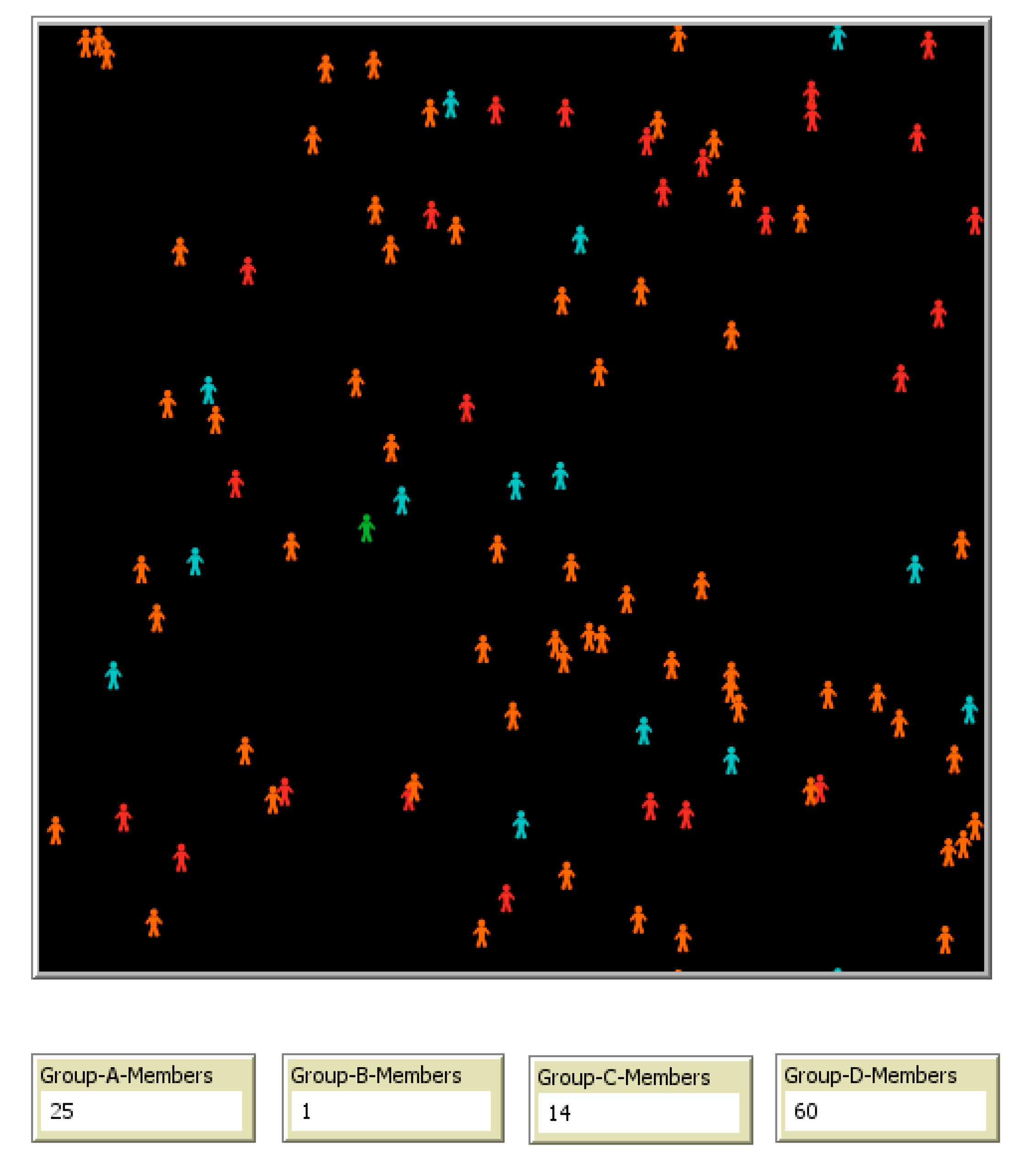
| Percentage of shareholders per Class of shareholders | xit | In this paper, we consider n = 4 classes of shareholders (i = A, B, C, D), defined in Section 3.2. . | |
| Residual value | RV | The cash flow resulted at the end-life of the investment project | |
| Realized capital market return | kMt | Random variable, normal distributed, with a mean and a finite standard deviation | |
| Realized internal rate of return | IRRt | Random variable, normal distributed, with a mean and a finite standard deviation | |
| Realized rate of return on assets | ROAt | In this paper, ROA = ROE | |
| Realized rate of return on equity | ROEt | In this paper, ROA = ROE | |
| Required rate of return on equity | ROE*t | ||
| Total assets | TAt | In this paper, TA = TE. Input in the model. | |
| Total equity | TEt | In this paper, TA = TE. Input in the model. | |
| Shareholders’ wealth | Wm |
| Financial Exercise (Year) | Phase | Content |
|---|---|---|
| 0 | ||
| 1 | 1.1 | The company records output results: ROE1 and NE1. |
| 1.2 | If NE1 ≤ 0, DIV1 = 0. Otherwise, the management (the controlling shareholder) anticipates Et−1(IRRt), respectively E1(IRR2) | |
| 1.3 | AGM: The management (the controlling shareholder) proposes a dividend policy: If E1(IRR2) ≥ E1(kM2), then: DIV1 = 0 If E1(IRR2) < E1(kM2), then: DIV1 = NE1 | |
| 1.4–1.5 | AGM: shareholders analyze the performance of the company at the present moment, as a proxy for the quality of the management’s decisions. We consider that, at this moment, the power remains in function. | |
| 2 | 2.1 | The company records output results: ROE2 and NE2. |
| 2.2 | If NE2 ≤ 0, DIV2 = 0. Otherwise, the management (the controlling shareholder) anticipates Et−1(IRRt), respectively E2(IRR3) | |
| 2.3 | AGM: The management (the controlling shareholder) proposes a dividend policy: If E2(IRR3) ≥ E2(kM3), then: DIV2 = 0 If E2(IRR3) < E2(kM3), then: DIV2 = NE2 | |
| 2.4 | AGM: shareholders analyze the performance of the company at the present moment, as a proxy for the quality of the management’s decisions: Notes: xtC = xt−1C + αt ·Mt (1 − xA − xB − xt−1C) = xt−1C (1 − αt ·Mt) + (1 − xA − xB)αt ·Mt | |
| 2.5 | AGM: vote: x2B + x2C ≤ 0.5, the management remains in power If x2B + x2C > 0.5, then the power is switched (the end of the discussion) | |
| 3 | 3.1 | The company records output results: ROE3 and NE3. |
| 3.2 | If NE3 ≤ 0, DIV3 = 0. Otherwise, the management (the controlling shareholder) anticipates Et−1(IRRt), respectively, E3(IRR4) | |
| … | … | |
| t | t.1 | The company records output results: ROEt and NEt. |
| t.2 | If NEt ≤ 0, DIVt = 0. Otherwise, the management (the controlling shareholder) anticipates Et−1(IRRt), respectively, Et(IRRt+1) | |
| t.3 | AGM: The management (the controlling shareholder) proposes a dividend policy: If Et(IRRt+1) ≥ Et(kMt+1), then: DIVt = 0 If Et(IRRt+1) < Et(kMt+1), then: DIVt = NEt | |
| t.4 | AGM: shareholders analyze the performance of the company at the present moment, as a proxy for the quality of the management’s decisions: Notes: xtC = xt−1C + αt · Mt (1 − xA − xB − xt–1C) = xt−1C (1 − αt · Mt) + (1 − xA − xB)αt · Mt | |
| t.5 | AGM: vote: xtB + xtC ≤ 0.5, the management remains in power If xtB + xtC > 0.5, then the power is switched (the end of the discussion; DSMBD is determined) | |
| … | … | … |
| … | … | … |
| Financial Exercise (Year) | Total Assets at the Beginning of the Period | Net Earnings | Return of Equity |
|---|---|---|---|
| 0 | TA−1 | NE0 | ROE0 |
| 1 | TA0 | ||
| 2 | |||
| 3 | … | ||
| … | … | … | … |
| n − 1 | … | … | |
| n |
| Financial Exercise | TAt | NEt | ROEt | Et–1(IRRt) | Et–1(kMt) | DIVt | xAt | xBt | xCt | xDt | APROEt | IRRt | kMt | bd | 1 − τ | ROEt* | Mt |
|---|---|---|---|---|---|---|---|---|---|---|---|---|---|---|---|---|---|
| (m.u.) | (m.u.) | (%) | (%) | (%) | (m.u.) | (%) | (%) | (%) | (%) | (%) | (%) | (%) | (%) | (%) | (%) | ||
| 0 | 1000 | 25.00 | 2.50 | 25.00 | 1.00 | 1.00 | 0.00 | 98.00 | 2.50 | ||||||||
| 1 | 1000 | 38.50 | 3.85 | 2.64 | 2.90 | 38.50 | 1.00 | 1.00 | 0.00 | 98.00 | 2.77 | ||||||
| 2 | 1000 | 56.00 | 5.60 | 9.32 | 0.65 | 0.00 | 1.00 | 1.00 | 0.00 | 98.00 | 3.17 | 2.38 | 2.90 | 10.00 | 90.00 | 2.86 | 20.00 |
| 3 | 1056 | −13.90 | −1.32 | 4.48 | 3.14 | 0.00 | 1.00 | 1.00 | 19.60 | 78.40 | 1.82 | 8.39 | 0.65 | 10.00 | 90.00 | 7.55 | 20.00 |
| … | … | … | … | … | … | … | … | … | … | … | … | … | … | … | … | … | … |
| Input | Notation | Level | Numerical Simulation | Distribution of the Variable | Remarks |
|---|---|---|---|---|---|
| Initial stock of total assets (equal to total equity) (initial wealth in our program) | TA0 | Fixed | 1000 | Constant | This level is configurable in slider “Initial-Total-Assets”. |
| Initial return on equity | ROE0 | Fixed | 2.5% | Constant | In the case of APROE calculations for the first periods (before the period of bad decisions), we have assumed also that ROE was equal to this level. |
| Expected market return | Et–1(kMt) | Random | Range between 0% and 5% | Normally distributed, with a mean of 2.5 and a standard deviation of 2.5. | At the beginning of each iteration, its value is changing. |
| Expected internal rate of return for the new projects | , ∀ t | Random | Range between 0% and 5% | Normally distributed with a mean of 2.5 and a standard deviation of 0.8 | eIRR in NetLogo |
| The impact of making bad decision | bd | Fixed | 0.1 | Constant | It can take values between 0 (this means the forecast is optimal) and 1 (this means that the forecast is totally inadequate). It can be set from the interface and ranges between 0%–100%. |
| The tolerance for the manager’s performance | τ | Fixed | 50% (but it can be set from the interface and ranges between 0%–100%) | Constant | It can be considered also as a resilience for changing the power. |
| The magnitude of interest to change the power | M | Random | 0.2 | Random (multi-values, each agent has its own value of this variable) | Range between 0% and 100% |
| S1 | S1-1 | S1-2 | S1-3 | S1-4 | S1-5 | S1-6 | S1-7 | |
|---|---|---|---|---|---|---|---|---|
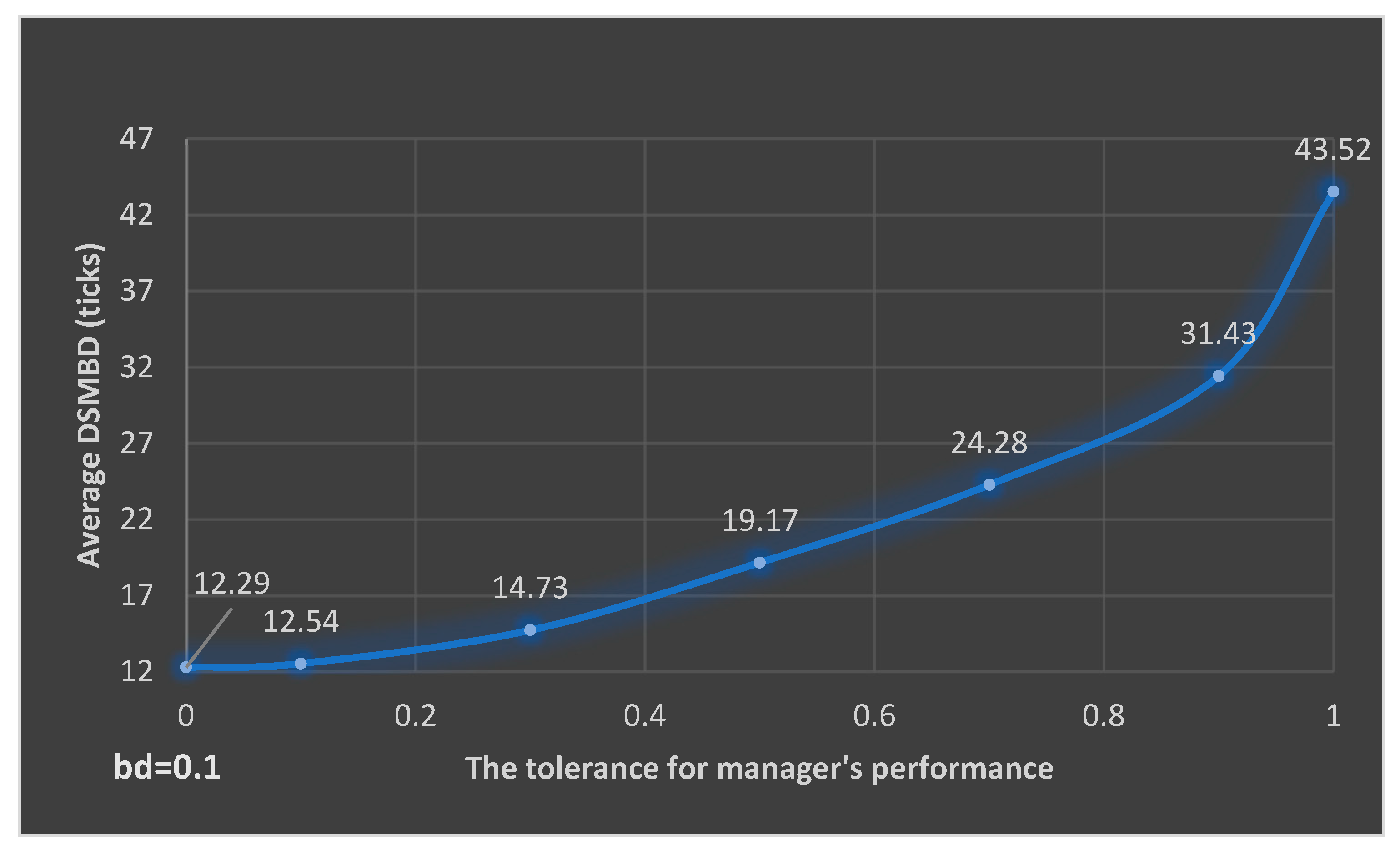
| Parameters | The tolerance for the manager’s performance (τ) | 0 | 0.1 | 0.3 | 0.5 | 0.7 | 0.9 | 1 |
| The impact of making bad decision (bd) | 0.1 | 0.1 | 0.1 | 0.1 | 0.1 | 0.1 | 0.1 | |
| Average DSMBD (ticks) | 12.29 | 12.54 | 14.73 | 19.17 | 24.28 | 31.43 | 43.52 | |
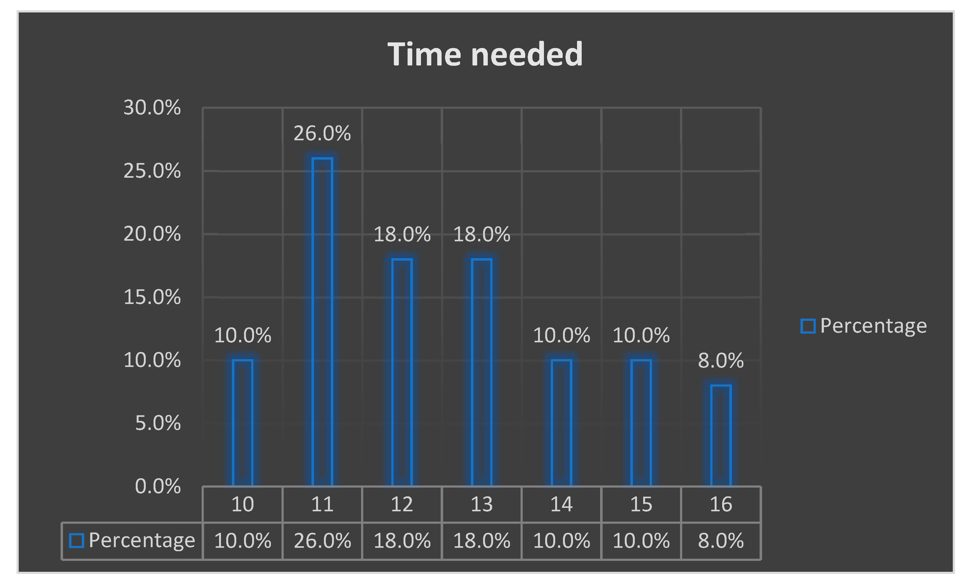
| DSMBD interval (min, max) | [10, 14] | [10, 16] | [11, 23] | [12, 27] | [15, 38] | [16, 39] | [24, 54] | |
| S1 | S1-8 | S1-9 | S1-10 | S1-11 | S1-12 | S1-13 | |
|---|---|---|---|---|---|---|---|
| Parameters | The tolerance for the manager’s performance (τ) | 0.5 | 0.5 | 0.5 | 0.5 | 0.5 | 0.5 |
| The impact of making bad decision (bd) | 0 | 0.3 | 0.5 | 0.7 | 0.9 | 1 | |
| Average DSMBD (ticks) | 20.26 | 19.05 | 17.73 | 16.92 | 16.31 | 16.04 | |
| DSMBD interval (min, max) | [14, 27] | [12, 27] | [12, 26] | [12, 25] | [12, 24] | [12, 20] | |
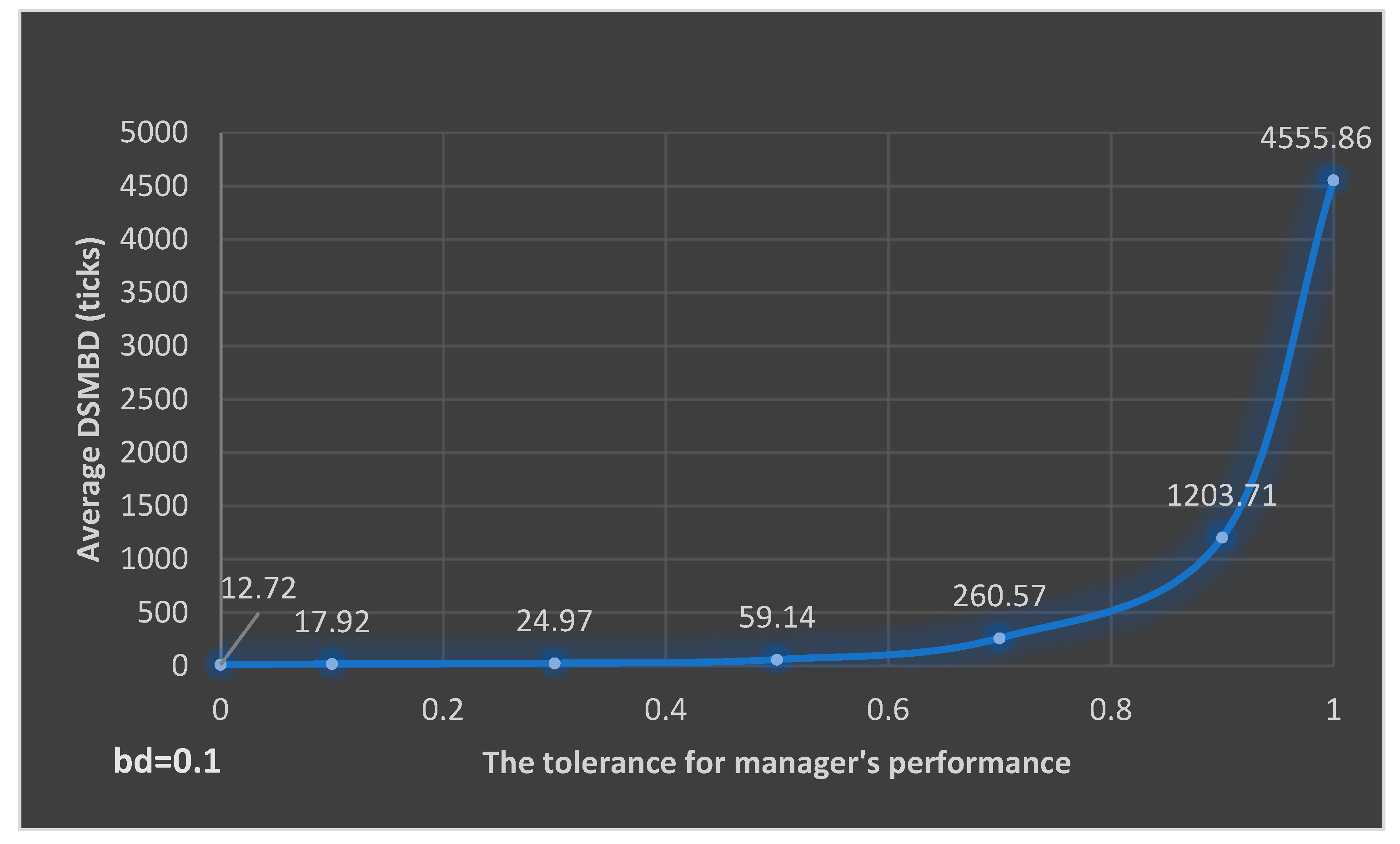
| S2 | S2-1 | S2-2 | S2-3 | S2-4 | S2-5 | S2-6 | S2-7 | |
|---|---|---|---|---|---|---|---|---|
| Parameters | The tolerance for the manager’s performance (τ) | 0 | 0.1 | 0.3 | 0.5 | 0.7 | 0.9 | 1 |
| The impact of making bad decision (bd) | 0.1 | 0.1 | 0.1 | 0.1 | 0.1 | 0.1 | 0.1 | |
| Average DSMBD (ticks) | 12.72 | 17.92 | 24.97 | 59.14 | 260.57 | 1203.71 | 4555.86 | |
| DSMBD interval (min, max) | [10, 15] | [10, 43] | [11, 85] | [12, 166] | [49, 741] | [263, 2252] | [933, 12489] | |
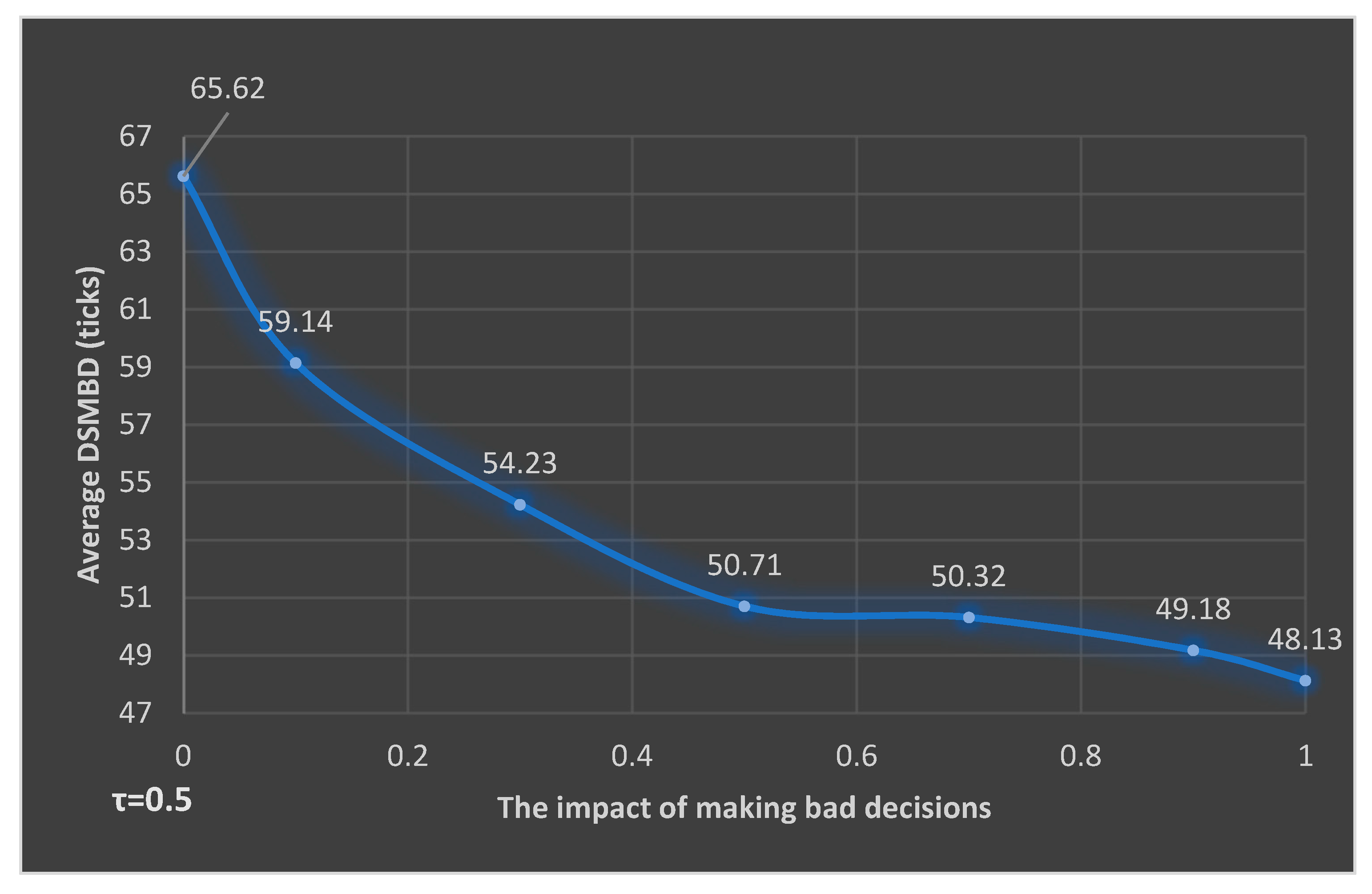
| S2 | S2-8 | S2-9 | S2-10 | S2-11 | S2-12 | S2-13 | |
|---|---|---|---|---|---|---|---|
| Parameters | The tolerance for the manager’s performance (τ) | 0.5 | 0.5 | 0.5 | 0.5 | 0.5 | 0.5 |
| The impact of making bad decision (bd) | 0 | 0.3 | 0.5 | 0.7 | 0.9 | 1 | |
| Average DSMBD (ticks) | 65.62 | 54.23 | 50.71 | 50.32 | 49.18 | 48.13 | |
| DSMBD interval (min, max) | [20, 171] | [12, 164] | [12, 144] | [12, 141] | [12, 138] | [12, 116] | |
© 2019 by the authors. Licensee MDPI, Basel, Switzerland. This article is an open access article distributed under the terms and conditions of the Creative Commons Attribution (CC BY) license (http://creativecommons.org/licenses/by/4.0/).
Share and Cite
Dragotă, V.; Delcea, C. How Long Does It Last to Systematically Make Bad Decisions? An Agent-Based Application for Dividend Policy. J. Risk Financial Manag. 2019, 12, 167. https://doi.org/10.3390/jrfm12040167
Dragotă V, Delcea C. How Long Does It Last to Systematically Make Bad Decisions? An Agent-Based Application for Dividend Policy. Journal of Risk and Financial Management. 2019; 12(4):167. https://doi.org/10.3390/jrfm12040167
Chicago/Turabian StyleDragotă, Victor, and Camelia Delcea. 2019. "How Long Does It Last to Systematically Make Bad Decisions? An Agent-Based Application for Dividend Policy" Journal of Risk and Financial Management 12, no. 4: 167. https://doi.org/10.3390/jrfm12040167
APA StyleDragotă, V., & Delcea, C. (2019). How Long Does It Last to Systematically Make Bad Decisions? An Agent-Based Application for Dividend Policy. Journal of Risk and Financial Management, 12(4), 167. https://doi.org/10.3390/jrfm12040167