Article

Forecasting Realized Volatility Using a Nonnegative Semiparametric Model

1
J.P. Morgan, 25 Bank Street, London E14 5JP, UK
2
School of Economics, Singapore Management University, Singapore 188065, Singapore
*
Author to whom correspondence should be addressed.
J. Risk Financial Manag. 2019, 12(3), 139; https://doi.org/10.3390/jrfm12030139
Submission received: 21 June 2019 / Revised: 25 August 2019 / Accepted: 26 August 2019 / Published: 29 August 2019
(This article belongs to the Special Issue Financial Econometrics)

Abstract

:
This paper introduces a parsimonious and yet flexible semiparametric model to forecast financial volatility. The new model extends a related linear nonnegative autoregressive model previously used in the volatility literature by way of a power transformation. It is semiparametric in the sense that the distributional and functional form of its error component is partially unspecified. The statistical properties of the model are discussed and a novel estimation method is proposed. Simulation studies validate the new method and suggest that it works reasonably well in finite samples. The out-of-sample forecasting performance of the proposed model is evaluated against a number of standard models, using data on S&P 500 monthly realized volatilities. Some commonly used loss functions are employed to evaluate the predictive accuracy of the alternative models. It is found that the new model generally generates highly competitive forecasts.

1. Introduction

Financial market volatility is an important input for asset allocation, investment, derivative pricing and financial market regulation. Not surprisingly, how to model and forecast financial volatility has been a subject of extensive research. Numerous survey papers are now available on the subject, with hundreds of reviewed research articles. Excellent survey articles on the subject include Bollerslev et al. (1992); Bollerslev et al. (1994); Ghysels et al. (1996); Poon and Granger (2003); and Shephard (2005).
In this vast literature, ARCH and stochastic volatility (SV) models are popular parametric tools. These two classes of models are motivated by the fact that volatilities are time-varying. Moreover, they offer ways to estimate past volatility and forecast future volatility from return data. In recent years, however, many researchers have argued that one could measure latent volatility by realized volatility (RV), see for example Andersen et al. (2001) (ABDL 2001 hereafter) and Barndorff-Nielsen and Shephard (2002), and then build a time series model for volatility forecasting using observed RV, see for example Andersen et al. (2003) (ABDL 2003 hereafter). An advantage of this approach is that “models built for the realized volatility produce forecasts superior to those obtained from less direct methods” (ABDL 2003). In an important study, ABDL (2003) introduced a new Gaussian time series model for logarithmic RV (log-RV) and established its superiority for RV forecasting over some standard methods based on squared returns. Their choice of modeling log-RV rather than raw RV is motivated by the fact that the logarithm of RV, in contrast to RV itself, is approximately normally distributed. Moreover, conditional heteroskedasticity is greatly reduced in log-RV.
Following this line of thought, in this paper we introduce a new time series model for RV. For the S&P 500 monthly RV, we show that although the distribution of log-RV is closer to a normal distribution than that of raw RV, normality is still rejected at all standard significance levels. Moreover, although conditional heteroskedasticity is reduced in log-RV, there is still evidence of remaining conditional heteroskedasticity. These two limitations associated with the logarithmic transformation motivate us to consider a more flexible transformation, that is, the so-called Tukey’s power transformation which is closely related to the well-known Box-Cox transformation. In contrast to the logarithmic transformation, Tukey’s power transformation or the Box-Cox transformation is generally not compatible with a normal error distribution as the support for the normal distribution covers the entire real line.1 This well-known truncation problem further motivates us to use nonnegative error distributions. The new model, which we call a Tukey nonnegative type autoregression (TNTAR), is flexible, parsimonious and has a simple forecast expression. Moreover, the numerical estimation of the model is very fast and can easily be implemented using standard computational software.
The new model is closely related to the linear nonnegative models described in Barndorff-Nielsen and Shephard (2001) and Nielsen and Shephard (2003). In particular, it generalizes the discrete time version of the nonnegative Ornstein-Uhlenbeck process of Barndorff-Nielsen and Shephard (2001) by (1) applying a power transformation to volatility; (2) leaving the dependency structure and the distribution of the nonnegative error term unspecified. Our work is also related to Yu et al. (2006) and Gonçalves and Meddahi (2011) where the Box-Cox transformation is applied to stochastic volatility and RV, respectively. The main difference between our model specification and theirs is that an unspecified (marginal) distribution with nonnegative support, instead of the normal distribution, is induced by the transformation. Moreover, our model is loosely related to Higgins and Bera (1992); Hentschel (1995) and Duan (1997) where the Box-Cox transformation is applied to ARCH volatility, and to Fernandes and Grammig (2006) and Chen and Deo (2004). Finally, our model is related to a recent study by Cipollini et al. (2006) where an alternative model with nonnegative errors is used for RV. The main difference here is that the dynamic structure for the transformed RV is linear in our model, whereas the dynamic structure for the RV is nonlinear in theirs.
Our proposed model is estimated using a two-stage estimation method. In the first stage, a nonlinear least squares procedure is applied to a nonstandard objective function. In the second stage a linear programming estimator is applied. The finite sample performance of the proposed estimation method is studied via simulations.
The TNTAR model is used to model and forecast the S&P 500 monthly RV and its out-of-sample performance is compared to a number of standard time series models previously used in the literature, including the exponential smoothing method and two logarithmic long-memory ARFIMA models. Under various loss functions, we find that our parsimonious nonnegative model generally generates highly competitive forecasts. While this paper considers the application of forecasting RV, there are a number of applications beyond financial data for which our model may be useful. For example, modeling and forecasting climatological or telecommunication time series may be interesting alternative applications for our nonnegative model.
While our model is related to several models in the literature, to the best of our knowledge, our specification is new in two ways. First, it is based on Tukey’s power transformation. Second, the distribution and functional form of its error component are partially unspecified. Moreover, the estimation method that we propose is new.
The rest of the paper is organized as follows. Section 2 motivates and presents the new model. In Section 3 a novel estimation method is proposed to estimate the parameters of the new model. In Section 4 the finite sample performance of the new method is studied via simulations. Section 5 describes the S&P 500 realized volatility data and the empirical results. In the same section we also outline the alternative models for volatility forecasting and present the loss functions used to assess their forecast performances. Finally, Section 6 concludes.

2. A Nonnegative Semiparametric Model

Before introducing the new TNTAR model, we first review two related time series models previously used in the volatility literature, namely, a simple nonnegative autoregressive (AR) model and the Box-Cox AR model.

2.1. Related Volatility Models

Barndorff-Nielsen and Shephard (2001) introduced the following continuous time model for financial volatility, σ 2 ( t ) ,
d σ 2 ( t ) = λ σ 2 ( t ) d t + d z ( λ t ) , λ > 0 .
In the above z is a Lévy process with independent nonnegative increments, which ensures the positivity of σ 2 ( t ) (see Equation (2) in Barndorff-Nielsen and Shephard 2001). Applying the Euler approximation to the continuous time model in (1) yields the following discrete time model
σ t + 1 2 = φ σ t 2 + u t + 1 ,
where φ = 1 λ and u t + 1 = z ( λ ( t + 1 ) ) z ( λ t ) is a sequence of independent identically distributed (i.i.d.) random variables whose distribution has a nonnegative support. A well known nonnegative random variable is the generalized inverse Gaussian, whose tails can be quite fat. Barndorff-Nielsen and Shephard (2001) discuss the analytical tractability of this model. In the case when u t + 1 is exponentially distributed, Nielsen and Shephard (2003) derive the finite sample distribution of a linear programming estimator for φ for the stationary, unit root and explosive cases.2 Simulated paths from model (2) typically match actual realized volatility data quite well. See, for example, Figure 1c in Barndorff-Nielsen and Shephard (2001). Unfortunately, so far little empirical evidence establishing the usefulness of this model has been reported.
Two restrictions seem to apply to model (2). First, since its errors are independent, conditional heteroskedasticity is not allowed for. The second restriction concerns the ratio of two successive volatilities. More specifically, from (2) it can be seen that σ t + 1 2 / σ t 2 is bounded from below by φ , almost surely, implying that σ t + 1 2 cannot decrease by more than 100 ( 1 φ ) % compared to σ t 2 . Since the AR parameter φ of the model typically is estimated using linear programming, in practice, this restriction is automatically satisfied. For instance, the full sample estimate of φ in our empirical study is 0.262 , implying that σ t 2 cannot decrease by more than 73.8% from one time period to the next. Indeed, 73.8% is the maximum percentage drop in successive monthly volatilities in the sample, which took place on November 1987.
In a discrete time framework, a popular parametric time series model for volatility is the lognormal SV model of Taylor (2007) given by
r t = σ t ε t ,
log σ t 2 = ( 1 φ ) μ + φ log σ t 1 2 + ϵ t ,
where r t is the return, σ t 2 is the latent volatility, and  ε t and ϵ t are two independent Gaussian noises. In this specification volatility clustering is modeled as an AR(1) for the log-volatility. The logarithmic transformation in (4) serves three important purposes: First, it ensures the positivity of σ t 2 . Second, it removes heteroskedasticity. Third, it induces normality.
 Yu et al. (2006) introduced a closely related SV model by replacing the logarithmic transformation in Taylor’s volatility Equation (4) with the more general Box-Cox transformation (Box and Cox 1964),
h ( σ t 2 , λ ) = ( 1 φ ) μ + φ h ( σ t 1 2 , λ ) + ϵ t ,
where
h ( x , λ ) = x λ 1 λ , λ 0 , log x , λ = 0 .
Compared to the logarithmic transformation, the Box-Cox transformation provides a more flexible way to improve normality and reduce heteroskedasticity. A nice feature of the Box-Cox AR model given by (5) and (6) is that it includes several standard specifications as special cases, including the logarithmic transformation ( λ = 0 ) and a linear specification ( λ = 1 ). In the context of SV, Yu et al. (2006) find empirical evidence against the logarithmic transformation. Chen and Deo (2004) and Gonçalves and Meddahi (2011) are interested in the optimal power transformation. In the context of RV, Gonçalves and Meddahi (2011) find evidence of non-optimality for the logarithmic transformation. They further report evidence of negative values of λ as the optimal choice for various data generating processes. Our empirical results reinforce this important conclusion, although our approach is very different.
While the above discrete time models have proven useful for modeling volatility, there is little documentation on their usefulness for forecasting volatility. Moreover, the Box-Cox transformation is known to be incompatible with a normal error distribution. This is the well-known truncation problem associated with the Box-Cox transformation in the context of Gaussianity.

2.2. Realized Volatility

In the ARCH or SV models, volatilities are estimated parametrically from returns observed at the same frequency. In recent years, however, it has been argued that one can measure volatility in a model-free framework using an empirical measure of the quadratic variation of the underlying efficient price process, that is, RV. RV has several advantages over ARCH and SV models. First, by treating volatility as directly observable, RV overcomes the well known curse-of-dimensionality problem in the multivariate ARCH or SV models. Second, compared to the squared return, RV provides a more reliable estimate of integrated volatility. This improvement in estimation naturally leads to gains in volatility forecasting.
Let R V t denote the RV at a lower frequency (say daily or monthly) and p ( t , k ) denote the log-price at a higher frequency (say intra-day or daily). Then R V t is defined by
R V t = k = 2 N p ( t , k ) p ( t , k 1 ) 2 ,
where N is the number of higher frequency observations in a lower frequency period.3
The theoretical justification for RV as a volatility measure comes from standard stochastic process theory, according to which the empirical quadratic variation converges to integrated variance as the infill sampling frequency tends to zero (ABDL 2001; Barndorff-Nielsen and Shephard 2002; Jacod 2017). The empirical method inspired by this consistency has recently become more popular with the availability of high-frequency data.
In a recent important contribution, ABDL (2003) find that a Gaussian long-memory model for the logarithmic daily realized variance provides more accurate forecasts than the GARCH(1,1) model and the RiskMetrics method of J.P. Morgan (1996). The logarithmic transformation is used since it is found that the distribution of logarithmic realized variance, but not raw realized variance, is approximately normal. In Table 1 we report (to 3 decimals) some summary statistics for monthly RV, log-RV and power-RV for the S&P 500 data in our empirical study over the period Jan 1946–Dec 2004, including the skewness, kurtosis, and p-value of the Jarque-Bera test statistic for normality.4 For RV, the departure from normality is overwhelming. While the distribution of log-RV is much closer to a normal distribution than that of RV, there is still strong evidence against normality.
To compare the conditional heteroskedasticities, in Figure 1 we plot squared OLS residuals ( ϵ ^ i t 2 , i = 1 , 2 , 3 ), obtained from AR(1) regressions for RV, log-RV and power-RV, respectively, against each corresponding explanatory variable (lagged RV, log-RV and power-RV). For ease of comparison, superimposed are smooth curves fitted using the LOESS method. It is clear that while the logarithmic transformation reduces the conditional heteroskedasticity there is still evidence of it in the residuals. The power transformation further reduces the conditional heteroskedasticity of RV. While the logarithmic transformation reduces the impact of large observations (extreme deviations from the mean), the second plot of Figure 1 suggests that it is not as effective as anticipated. In contrast, the power transformation with a negative power parameter is able to reduce the impact of large observations further. Thus, the results indicate that there is room for further improvements over the logarithmic transformation. A more detailed analysis of the S&P 500 data is provided in Section 5.

2.3. The Model

In this paper, our focus is on modeling and forecasting RV. To this end, let us first consider the RV version of model (5),
h ( R V t , λ ) = α + β h ( R V t 1 , λ ) + ϵ t ,
where ϵ t is a sequence of independent N ( 0 , σ ϵ 2 ) distributed random variables and h ( x , λ ) is given by (6).
If λ 0 , we may rewrite (8) as
R V t λ = ( 1 + λ α ) + β ( R V t 1 λ 1 ) + λ ϵ t ,
where R V t λ is a simple power transformation. A special case of (9) is a linear Gaussian AR(1) model, obtained when λ = 1 :
R V t = ( 1 + α β ) + β R V t 1 + ϵ t .
If λ = 0 in (8), we have the log-linear Gaussian AR(1) model previously used in the literature:
log R V t = α + β log R V t 1 + ϵ t .
While the specification in (8) is more general than the log-linear Gaussian AR(1) model (11), it has a serious drawback. In general, solving for R V t , the right hand side of (9) has to be nonnegative with probability one or almost surely (a.s.). This requirement is violated since a normal error distribution has a support covering the entire real line.
This drawback motivates us to explore an alternative model specification for RV. Our proposed nonnegative TNTAR model is of the form
R V t λ = φ R V t 1 λ + u t , t = 2 , 3 ,
with the power parameter λ 0 , AR parameter φ > 0 and (a.s.) positive initial value R V 1 . The errors u t driving the model are nonnegative, possibly non-i.i.d., random variables. In the simplest case, u t is assumed to be a sequence of m-dependent, identically distributed, continuous random variables with nonnegative support [ η , ) , for some unknown η 0 .5 It is assumed that m N is finite and potentially unknown. Hence, the distribution and functional form of u t is partially unspecified. We expect φ R V t 1 λ to be the dominating component in (12) and do not model u t parametrically.
The power transformation R V t λ is closely related to John W. Tukey’s ladder of power transformations for linearizing data (Tukey 1977), partially illustrated in (13) below:
1 x 3 1 x 2 1 x 1 x log x x x x 2 x 3 .
The nonnegative restriction on the support of the error distribution ensures the positivity of R V t λ . Hence, our model does not suffer from the truncation problem of the classical Box-Cox model (8). As the distribution of u t is left unspecified, some very flexible tail behavior is allowed for. Consequently, the drawback in the Box-Cox AR model (8) is addressed in the proposed TNTAR model (12).
In the classical Box-Cox model, the transformation parameter λ is required to induce linearity and normality and at the same time eliminate conditional heteroskedasticity. These are too many requirements for a single parameter. In our model, the role of the Tukey-type power transformation is to improve linearity and reduce conditional heteroskedasticity, not to induce normality. To illustrate this, suppose that a square root transformation is applied with λ = 1 / 2 in (12), then R V t = φ 2 R V t 1 + 2 φ R V t 1 u t + u t 2 and the conditional variance of raw R V is time-varying.6 An intercept in the model is superfluous because the support parameter η can be strictly positive. Our model echoes (8), with the normal distribution replaced by a nonnegative distribution. If  λ = 1 and its errors are i.i.d., our model becomes the discrete time version of Equation (2) in Barndorff-Nielsen and Shephard (2001). In general, the distributional and functional form is not assumed to be known for the error component. Hence, the TNTAR model combines a parametric component for the persistence with a nonparametric component for the error. On the one hand, the new model is highly parsimonious. In particular, there are only two parameters that need to be estimated for the purpose of volatility forecasting, namely φ and λ . On the other hand, the specification is sufficiently flexible for modeling the error.
As mentioned earlier, there exists a lower bound for the percentage change in volatility in model (2). A similar bound applies to our model. It is easy to show that R V t / R V t 1 φ 1 / λ if λ < 0 (upper bound) and  R V t / R V t 1 φ 1 / λ if λ > 0 (lower bound). Typical estimated values of φ and λ in (12) for our empirical study are 0.639 and −0.278, respectively, suggesting that R V t cannot increase by more than 500% from one time period to the next. As we will see later, our proposed estimator for λ depends on the ratios of successive RV’s and hence the bound is endogenously determined.

3. Robust Estimation and Forecasting

In this section we consider the estimation of the parameters φ and λ and a one-step-ahead forecast expression, for the TNTAR model. First, we consider the special case when λ is assumed to be known. Some common power transformations include λ = 1 / n (the nth root transformation) and its reciprocal, λ = 1 / n . Second, we consider the more general case when both φ and λ are unknown and need to be estimated. We then examine the finite sample performance of the proposed estimation method via simulations.

3.1. Robust Estimation of φ

If the true value of the power transformation parameter is known, a natural estimator for φ in (12) given the sample R V 1 , , R V T of size T and the nonnegativity of the errors is
φ ^ T = min R V 2 λ R V 1 λ , , R V T λ R V T 1 λ = φ + min u 2 R V 1 λ , , u T R V T 1 λ .
The estimator φ ^ T in (14) can be viewed as the solution to a linear programming problem. Because of this, we will refer to it as a linear programming estimator (LPE). This estimator is also the conditional (on R V 1 ) maximum likelihood estimator (MLE) of φ when the errors in (12) are i.i.d. exponentially distributed random variables, cf. Nielsen and Shephard (2003). Interestingly, the LPE is strongly consistent for more general error specifications, including heteroskedasticity and m-dependence. It is robust in the sense that its consistency conditions allow for certain model misspecifications in u t . For example, the order of m-dependence in the error sequence and the conditional distribution of R V t may be incorrectly specified. Moreover, the LPE is strongly consistent even under quite general forms of heteroskedasticity and structural breaks. For a more detailed account of the properties of the LPE, see Preve (2015).
Like the ordinary least squares (OLS) estimator for φ , the LPE is distribution-free in the sense that its consistency does not rely on a particular distributional assumption for the error component. However, the LPE is in many ways superior to the OLS estimator. For example, its rate of convergence can be faster than O p ( T 1 / 2 ) even for φ < 1 , whereas the rate of covergence for the OLS estimator is faster than O p ( T 1 / 2 ) only for φ 1 , see Phillips (1987). Furthermore, unlike the OLS estimator the consistency conditions for the LPE do not involve the existence of any higher order moments.
Under additional technical conditions, Davis and McCormick (1989) and Feigin and Resnick (1992) obtain the limiting distribution of a LPE for which (14) appear as a special case when λ = 1 and the errors are i.i.d.. The authors show that the accuracy of the LPE depends on the index of regular variation at zero (or infinity) of the error distribution function. For example, for standard exponential errors, the index of regular variation at zero is 1 and the LPE converges to φ at the rate of O p ( T 1 ) . In general, a difficulty in the application of the limiting distribution is that the index of regular variation at zero appears both in a normalizing constant and in the limit. Datta and McCormick (1995) avoid this difficulty by establishing the asymptotic validity of a bootstrap scheme based on the LPE.
It is readily verified that the LPE in (14) is positively biased and stochastically decreasing in T, that is, φ < φ ^ T 2 φ ^ T 1 a.s. for any T 1 < T 2 .7 Hence, the accuracy of the LPE either remains the same or improves as the sample size increases (cf. Figure 2).
To illustrate the robustness of the LPE, consider a covariance stationary AR(1) model
R V t = φ R V t 1 + u t , t = 0 , ± 1 , ± 2 , ,
under the possible misspecification
u t = ϵ t + i = 1 m ψ i ϵ t i ,
where ϵ t is a sequence of non-zero mean i.i.d. random variables. For  m > 0 the (identically distributed) errors u t are serially correlated. In this setting the OLS estimator for φ is inconsistent while the LPE remains consistent. In the first panel of Figure 2 we plot 100 observations simulated from the nonnegative ARMA(1,1) model, R V t = φ R V t 1 + ϵ t + ψ ϵ t 1 with φ = 0.5 , ψ = 0.75 and standard exponential noise. In the second panel of Figure 2 we plot the sample paths of the recursive LPEs and OLS estimates for φ obtained from the simulated data. In each iteration, a new observation is added to the sample used for estimation. It can be seen that the LPEs quickly approach the true value φ , whereas the OLS estimates do not. Moreover, the OLS estimates fluctuate much more than the LPEs when the sample size is small, suggesting that the LPE is less sensitive to extreme deviations from the mean than the OLS estimator in small samples.
We now list simple assumptions under which the consistency of the LPE in (14) holds. More general assumptions, allowing for an unknown number of unknown breaks in the error mean and variance, under which the LPE converges to φ for a known λ are given in Preve (2015).
Assumption 1.
The power transformation parameter λ 0 in (12) is known. The AR parameter φ > 0 , and the initial value R V 1 is a.s. positive. The errors u t driving the autoregression form a sequence of m-dependent, identically distributed, nonnegative continuous random variables. The order, m, of the dependence is finite.
Assumption 1 allows for various kinds of m-dependent error specifications, with  m N potentially unknown. For example, serially correlated finite-order MA specifications. Since the functional form and distribution of u t are taken to be unknown, the formulation is nonparametric.
Assumption 2.
The error component in (12) satisfies P ( c 1 < u t < c 2 ) < 1 for all 0 < c 1 < c 2 < .
It is important to point out that Assumption 2 is satisfied for any error distribution with unbounded nonnegative support.
Theorem 1.
Suppose that Assumptions 1 and 2 hold. Then the LPE in (14) is strongly consistent for φ in (12). That is, φ ^ T converges to φ a.s. as T tends to infinity.
The convergence of φ ^ T is almost surely (and, hence, also in probability). Our interest is in forecasting raw RV, not the power transformation of RV in (12). Let R V ^ T + 1 denote a forecast of R V T + 1 made at time T. A simple approximation to the optimal mean squared error, one-step-ahead, forecast of R V T + 1 at time T is given by the sample average
R V ^ T + 1 = 1 T 1 i = 2 T φ ^ T R V T λ + u ^ i 1 / λ ,
where u ^ i = R V i λ φ ^ T R V i 1 λ converges to u i in distribution as T tends to infinity under Assumptions 1 and 2.

3.2. Estimation of φ and λ

In practice, we usually do not know the true value of λ . In this section we propose an LPE based two-stage estimation method for φ and λ in the TNTAR model (12). In doing so, we also establish a general expression for its one-step-ahead forecast. The estimators are easily computable using standard computational software such as Matlab.
Joint estimation of φ and λ is non-trivial, even under certain parametric and simplifying assumptions for u t . For example, even in the simple case when u t is a sequence of independent exponentially distributed random variables it appears that the MLEs of φ and λ are inconsistent. Because of this we propose an estimation method based on the LPE for φ .
In our LPE based two-stage estimation method, we first choose λ ^ T to minimize the sum of squared one-step-ahead prediction errors:
λ ^ T = min l 1 T 1 t = 2 T R V t R V ^ t ( l ) 2 ,
where
R V ^ t ( l ) = 1 T 1 i = 2 T φ ^ T ( l ) R V t 1 l + u ^ i ( l ) 1 / l ,
with
φ ^ T ( l ) = min R V t l R V t 1 l t = 2 T and u ^ i ( l ) = R V i l φ ^ T ( l ) R V i 1 l ,
respectively. Although our estimator for λ looks like the standard nonlinear least squares (NLS) estimator of Jennrich (1969), the two approaches are quite different because in our model an explicit expression for E ( R V t R V t 1 ) is not available. In fact, the NLS estimators of λ and φ , that minimizes t = 2 T ( R V t l p R V t 1 l ) 2 , always take values of 0 and 1, respectively and hence are inconsistent.
The intuition behind the proposed estimation method is that we expect R V ^ t ( λ ^ T ) to be close to E ( R V t R V t 1 ) for large values of T. This is not surprising since the TNTAR model (12) implies that
R V t = φ R V t 1 λ + u t 1 / λ ,
and hence
E ( R V t R V t 1 ) = E φ R V t 1 λ + u t 1 / λ R V t 1 .
In the second stage, we use the LPE to estimate φ . More specifically,
φ ^ T = φ ^ T ( λ ^ T ) = min R V t λ ^ T R V t 1 λ ^ T t = 2 T .
while we minimize the sum of squared one-step-ahead prediction errors when estimating λ , other criteria, such as minimizing the sum of absolute one-step-ahead prediction errors, can be used. We have experimented with absolute prediction errors using the S&P 500 data and found that our out-of-sample forecasting results for the TNTAR model are quite insensitive to the choice of the objective function in the estimation stage. However, the objective function with squared prediction errors performs better in simulations.
It is beyond the scope of this paper to derive asymptotic properties for the two-stage estimators. However, under primitive assumptions, the consistency of λ ^ T and φ ^ T can be established using the fundamental consistency result for extremum estimators. Moreover, under high-level assumptions, the martingale central limit theorem can be used to establish the asymptotic distribution of λ ^ T .
With an estimated λ and φ , a general one-step-ahead semiparametric forecast expression for the TNTAR model is given by
R V ^ T + 1 = 1 T 1 i = 2 T φ ^ T R V T λ ^ T + u ^ i 1 / λ ^ T ,
where u ^ i = R V i λ ^ T φ ^ T R V i 1 λ ^ T is the residual at time i. Of course, in line with Granger and Newbold (1976), several forecasts of R V T + 1 may be considered. For example, one could base a forecast on the well known approximation E [ h ( y ) ] h [ E ( y ) ] using h ( y ) = y 1 / λ . However, this approximation does not take into account the nonlinearity of h ( y ) .8

4. Monte Carlo Studies

We now examine the performance of our estimation method via simulations. We consider two experiments in which data are generated by the nonnegative model
R V t λ = φ R V t 1 λ + u t u t = ϵ t + ψ ϵ t 1 ,
with i.i.d. standard exponential driving noise ϵ t .
In the first Monte Carlo experiment λ is assumed to be known and we only estimate φ using the LPE in (14). In this case the consistency is robust to the first-order moving average specification of u t . Hence, we simulate data from the model with the value of ψ being different from zero. Specifically, the parameter values are set to λ = 0.25 and ψ = 0.75 . The values of φ considered are 0.25 , 0.5 and 0.75 , respectively. In the second experiment λ is assumed to be unknown and is estimated together with φ using the proposed two-stage method. The parameter values are λ = 0.5 and 0.25 , φ = 0.5 and 0.75 , and  ψ = 0 .
The values chosen for λ and φ in the two experiments are empirically realistic (cf. the results of Section 5). We consider sample sizes of T = 200 ,   400 and 800 in both experiments. The sample size of 400 is close to the smallest sample size used for estimation in our empirical study, while the sample size of 800 is close to the largest sample size in the study. Simulation results based on 100,000 Monte Carlo replications are reported in Table 2 and Table 3. Several interesting results emerge from the tables. First, the smaller the value of T, the greater the empirical bias in φ ^ T in the first experiment and in λ ^ T and φ ^ T in the second experiment. Second, as T increases, the empirical mean squared error of φ ^ T in the first experiment, and those of λ ^ T and  φ ^ T in the second experiment, decreases. It may be surprising to see that the bias of φ ^ T can be negative in the second experiment. Here the negative bias arises because λ is estimated. In sum, it seems that the proposed estimation method works well, especially when T is reasonably large.

5. An Empirical Study

We also study the performance of the proposed model for forecasting actual RV relative to popular existing models. Before we report empirical results, we first review some alternative models and criteria to evaluate the performance of different models.

5.1. Alternative Models

Numerous models and methods have been applied to forecast stock market volatility. For example, ARCH-type models are popular in academic publications and RiskMetrics is widely used in practice. Both methods use returns to forecast volatility at the same frequency. However, since the squared return is a noisy estimator of volatility ABDL (2003) instead consider RV and present strong evidence to support time series models based directly on RV in terms of forecast accuracy. Motivated by their empirical findings, we compare the forecast accuracy of the TNTAR model against four alternative models, all based on RV: (1) the linear Gaussian AR(1) model (AR); (2) the log-linear Gaussian AR(1) model (log-AR); (3) the logarithmic autoregressive fractionally integrated moving average (ARFIMA) model; (4) the heterogeneous autoregressive (HAR) model. We also compare the performance of our model against the exponential smoothing method, a RV version of RiskMetrics. The AR and log-AR models are defined by (10) and (11), respectively. We now review the exponential smoothing method, the ARFIMA model, and the HAR model.

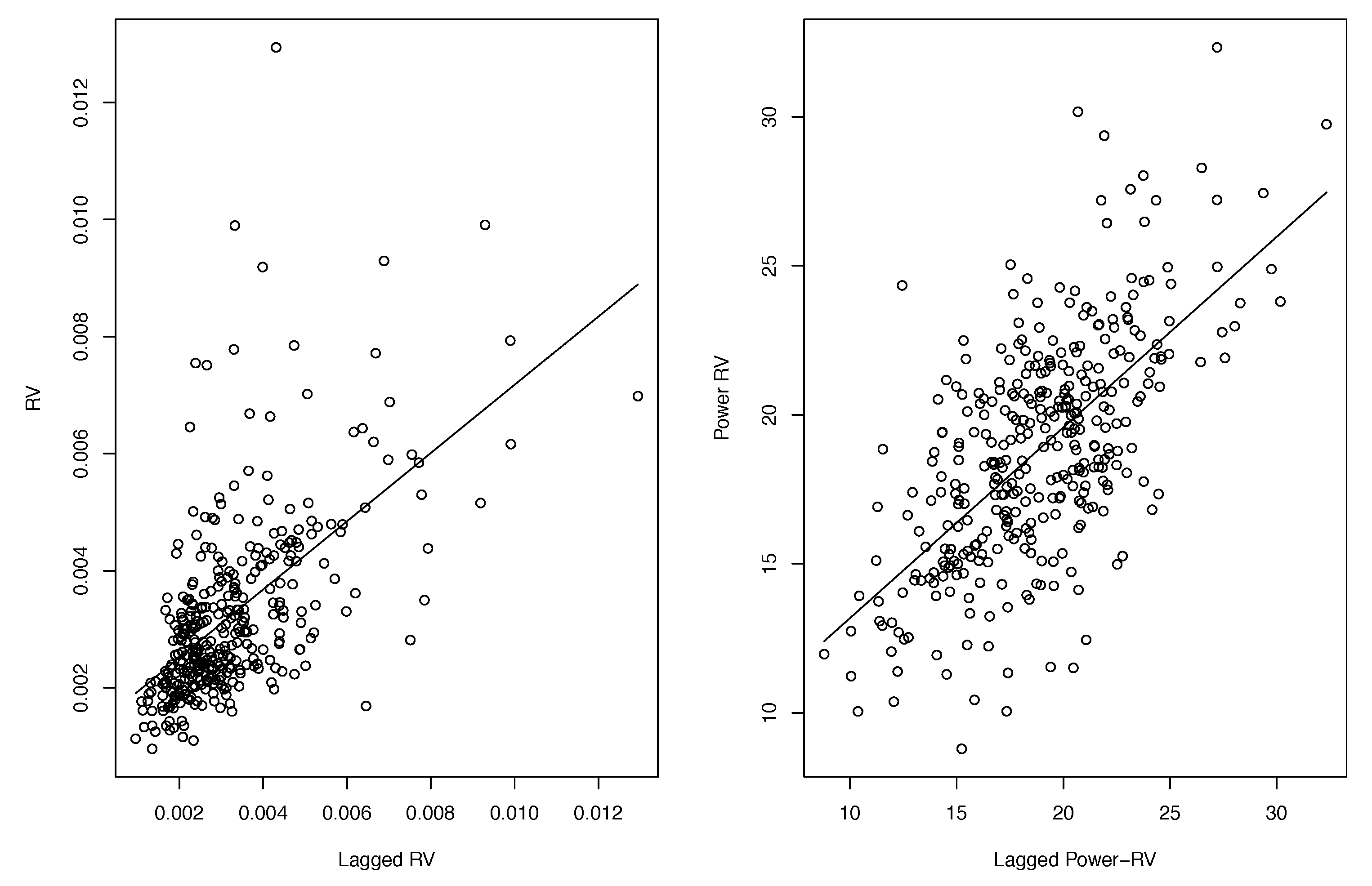
5.1.1. Exponential Smoothing

Exponential smoothing (ES) is a simple method of forecasting, where the one-step-ahead forecast of R V T + 1 at time T is given by
R V ^ T + 1 = ( 1 α ) R V T + α R V ^ T = ( 1 α ) i = 0 T 1 α i R V T i ,
with 0 < α < 1 .
The exponential smoothing formula can be understood as the RV version of RiskMetrics, where the squared return, r T 2 , is replaced by R V T . Under the assumption of conditional normality of the return distribution, r T 2 is an unbiased estimator of σ t 2 . RiskMetrics recommends α = 0.94 for daily data and α = 0.97 for monthly data.
To see why the squared return is a noisy estimator of volatility even under the assumption of conditional normality of the return distribution, suppose that r t follows (3). Conditional on σ t , it is easy to show that (Lopez 2001)
P r t 2 1 2 σ t 2 , 3 2 σ t 2 = 0.259 .
This implies that with a probability close to 0.74 the squared return is at least 50% greater, or at most 50% smaller, than the true volatility. Not surprisingly, Andersen and Bollerslev (1998) find that RiskMetrics is dominated by models based directly on RV. For this reason, we do not use RiskMetrics directly. Instead, we use (17) with α = 0.97 , which assigns a weight of 3% to the most recently observed RV. We remark that the forecasting results of Section 5 were qualitatively left unchanged when other values for α were used.

5.1.2. ARFIMA( p , d , q )

Long range dependence is a well documented stylized fact for volatility of many financial time series. Fractional integration has previously been used to model the long range dependence in volatility and log-volatility. The autoregressive fractionally integrated moving average (ARFIMA) was considered as a model for logarithmic RV in ABDL (2003) and Deo et al. (2006), among others. In this paper, we consider two parsimonious ARFIMA models for log-RV, namely, an ARFIMA( 0 , d , 0 ) and an ARFIMA( 1 , d , 0 ).
The ARFIMA( p , d , 0 ) model for log-RV is defined by
( 1 β 1 B β p B p ) ( 1 B ) d ( log R V t μ ) = ε t ,
where the parameters μ , β 1 , , β p and the memory parameter d are real valued, and  ε t is a sequence of independent N ( 0 , σ ε 2 ) distributed random variables.
Following a suggestion of a referee, we estimate all the parameters of the ARFIMA model using an approximate ML method by minimizing the sum of squared one-step-ahead prediction errors. See Beran (1995), Chung and Baillie (1993), and Doornik and Ooms (2004) for detailed discussions about the method and for Monte Carlo evidence supporting it. Compared to the exact ML method of Sowell (1992), there are two advantages to the approximate ML method. First, it does not require d to be less than 0.5. Second, it has smaller finite sample bias. Compared to the semi-parametric methods, it is also more efficient.9 The one-step-ahead forecast of R V T + 1 at time T of an ARFIMA( p , d , 0 ) for log-RV with p = 0 is given by
R V ^ T + 1 = exp μ ^ j = 0 T 1 π ^ j log R V T j μ ^ + σ ^ ε 2 2 ,
and with p = 1 by
R V ^ T + 1 = exp μ ^ + β ^ log R V T μ ^ + j = 1 T 1 π ^ j β ^ log R V T j μ ^ log R V T j + 1 μ ^ + σ ^ ε 2 2 ,
where
π ^ j = Γ j d ^ Γ j + 1 Γ d ^ ,
and Γ ( · ) denotes the gamma function.

5.1.3. HAR

The HAR model proposed by Corsi (2009) is one of the most popular models for forecasting volatility. Given that we will forecast monthly RV in the empirical study, we modify the original HAR model with monthly, quarterly and yearly components. The original HAR model was proposed to model daily RV. We apply the modified model to raw RV (HAR) and to log-RV (log-HAR). The model for raw RV can be expressed as
R V t = β 0 + β 1 R V t 1 m + β 2 R V t 1 q + β 3 R V t 1 y + ϵ t ,
where the parameters β 0 , , β 3 are real valued, R V t is the realized volatility of month t, and  R V t 1 m = R V t 1 , R V t 1 q = 1 3 i = 1 3 R V t i , R V t 1 y = 1 12 i = 1 12 R V t i denote the monthly, quarterly and yearly lagged RV components, respectively. This specification of RV parsimoniously captures the high persistence observed in our empirical study. The one-step-ahead forecast of R V T + 1 at time T is given by
R V ^ T + 1 = β ^ 0 + β ^ 1 R V T + β ^ 2 3 i = 1 3 R V T + 1 i + β ^ 3 12 i = 1 12 R V T + 1 i .
The corresponding forecast of the HAR model in (19) for log-RV is
R V ^ T + 1 = exp β ^ 0 + β ^ 1 log R V T + β ^ 2 3 i = 1 3 log R V T + 1 i + β ^ 3 12 i = 1 12 log R V T + 1 i + σ ^ ϵ 2 2 ,
where σ ^ ϵ 2 is the estimated variance of the independent N ( 0 , σ ϵ 2 ) distributed errors ϵ t .

5.2. Forecast Accuracy Measures

It is not obvious which accuracy measure is more appropriate for the evaluation of the out-of-sample performance of alternative time series models. Rather than making a single choice, we use four measures to evaluate forecast accuracy, namely, the mean absolute error (MAE), the mean absolute percentage error (MAPE), the mean square error (MSE) and the mean square percentage error (MSPE). Let R V ^ i t denote the one-step-ahead forecast of R V t at time t 1 of model i and define the accompanying forecast error by e i t = R V t R V ^ i t . The four accuracy measures are defined, respectively, by
MAE = 1 P t = 1 P | e i t | , MAPE = 100 P t = 1 P e i t R V t , MSE = 1 P t = 1 P e i t 2 , MSPE = 100 P t = 1 P e i t R V t 2 ,
where P is the length of the forecast evaluation period.
An advantage of using MAE instead of MSE is that it has the same scale as the data. The MAPE and the MSPE are scale independent measures. For a comprehensive survey on these and other forecast accuracy measures see Hyndman and Koehler (2006).
When calculating the forecast error, it is implicitly assumed that R V t is the true volatility at time t. However, in reality the volatility proxy R V t is different from the true, latent, volatility. Several recent papers discuss the implications of using noisy volatility proxies when comparing volatility forecasts under certain loss functions. See, for example, Andersen and Bollerslev (1998); Hansen and Lunde (2006) and Patton (2011). The impact is found to be particularly large when the squared return is used as a proxy for the true volatility, but diminishes with the approximation error. In this paper, the true (monthly) volatility is approximated by the RV using 22 (daily) squared returns. As a result, the approximation error is expected to be considerably smaller than in the case of using a single squared return.

5.3. Data

The data used in this paper consists of daily closing prices for the S&P 500 index over the period 2 January 1946–31 December 2004, covering 708 months and 15,054 trading days. We measure the monthly volatility using realized volatility calculated from daily data. Denote the log-closing price on the k’th trading day in month t by p ( t , k ) . Assuming there are T t trading days in month t, we define the monthly RV as
R V t = 1 T t k = 2 T t p ( t , k ) p ( t , k 1 ) 2 , t = 1 , , 708
where 1 / T t serves the purpose of standardization.
In order to compare the out-of-sample predictive accuracy of the alternative models, we split the time series of monthly RV into two subsamples. The first time period is used for the initial estimation. The second period is the hold-back sample used for forecast evaluation. When computing the forecasts we use a recursive scheme, where the size of the sample used for parameter estimation successively increases as new forecasts are made. The time series plot of monthly RV for the entire sample is shown in Figure 3, where the vertical dashed line indicates the end of the initial sample period used for estimation in our first forecasting exercise.
Table 4 shows the sample mean, maximum, skewness, kurtosis, the p-value of the JB test statistic for normality, and the first three sample autocorrelations of the entire sample for RV and log-RV. For RV, the sample maximum is 0.026 which occurred in October 1987. The sample kurtosis is 28.791 indicating that the distribution of RV is non-Gaussian. In contrast, log-RV has a much smaller kurtosis (3.657) and is less skewed (0.389). It is for this reason that we include Gaussian time series models for log-RV in the exercise. However, a formal test for normality via the JB statistic rejects the null hypothesis of normality of log-RV, suggesting that further improvements over log-linear Gaussian approaches are possible.
Higher order sample autocorrelations are in general slowly decreasing and not statistically negligible, indicating that RV and log-RV are predictable. To test for possible unit roots, augmented Dickey-Fuller (ADF) test statistics were calculated. The ADF statistic for the sample from 1946 to 2004 is 5.69 for RV and 5.43 for log-RV, which is smaller than 2.57 , the critical value at the 10% significance level. Hence, we reject the null hypothesis that RV or log-RV has a unit root.

5.4. Empirical Results

Each alternative model was fitted to the in-sample RV data and used to generate one-step-ahead out-of-sample forecasts.10 Following a suggestion of a referee, we also included a standard GARCH(1,1) (sGARCH) and a realized GARCH(1,1) with a log-linear specification (realGARCH), Hansen et al. (2012).11 Since a forecast frequency of one month is sufficiently important in practical applications, we focus on one-step-ahead forecasts in this paper. However, multi-step-ahead forecasts can be obtained in a similar manner.
We perform two out-of-sample forecasting exercises. In both exercises, we use the recursive scheme, where the size of the sample used to estimate the alternative models grows as we make forecasts for successive observations.12 More precisely, in the first exercise, we first estimate all the alternative models with data from the period January 1946–June 1975 and use the estimated models to forecast the RV of July 1975. We then estimate all models with data from January 1946–July 1975 and use the model estimates to forecast the RV of August 1975. This process (an expanding window of initial size 354) is repeated until, finally, we estimate the models with data from January 1946–November 2004. The final model estimates are used to forecast the RV of December 2004, the last observation in the sample.

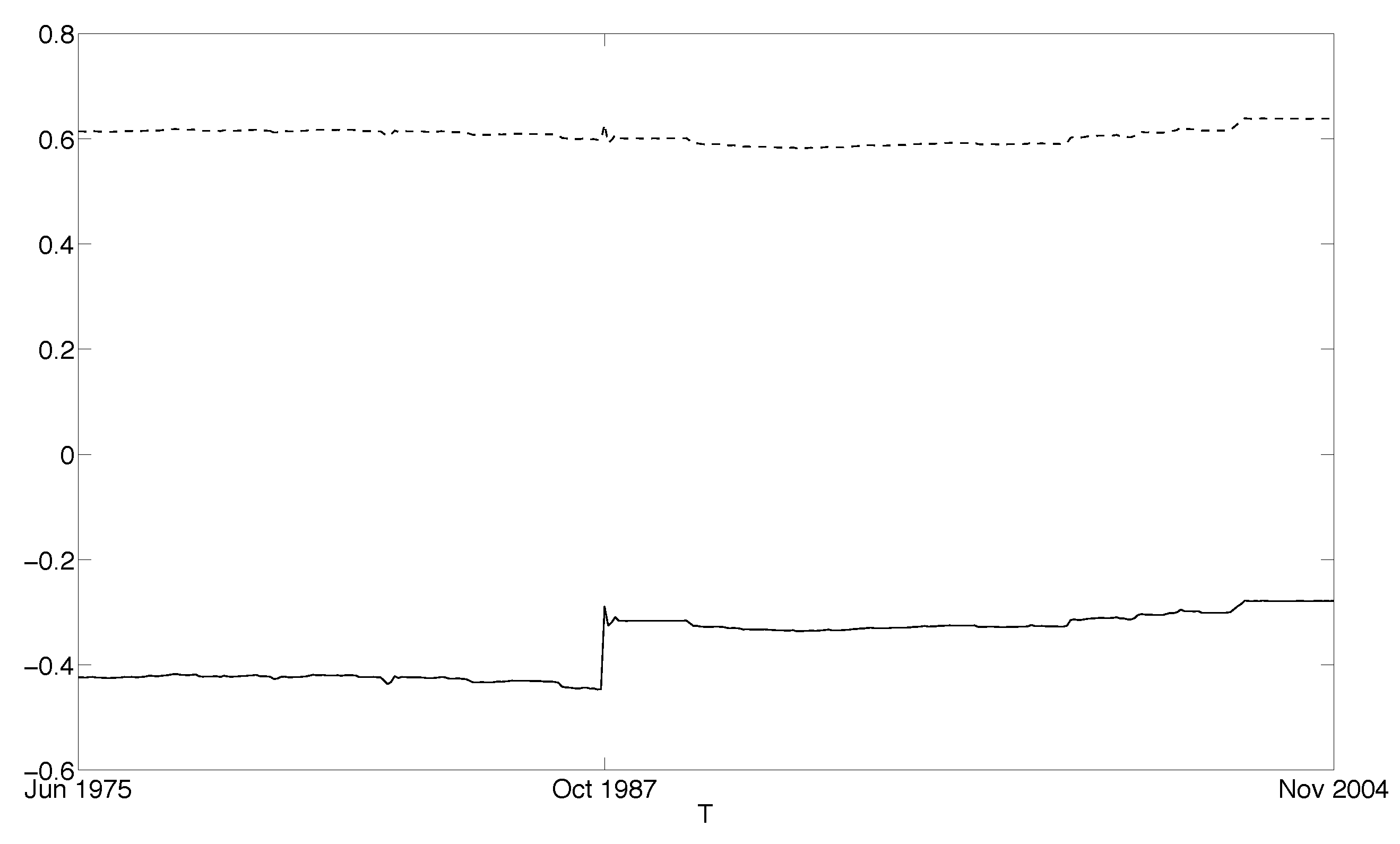
5.4.1. Sample including the 1987 Crash

In the first exercise, the first month for which an out-of-sample volatility forecast is obtained is July 1975. In total 354 monthly volatilities are forecasted, including the volatility of October 1987 when the stock market crashed and the RV is 0.026.
In Figure 4, we plot the monthly RV and the corresponding one-month-ahead TNTAR forecasts for the out-of-sample period, July 1975 to December 2004. It seems that the TNTAR model captures the overall movements in RV reasonably well. The numerical computation of the 354 forecasts is fast and takes less than five minutes on a standard desktop computer.
In Figure 5, we plot the recursive estimates, λ ^ T and φ ^ T . While λ ^ T takes values from 0.45 to 0.28 , φ ^ T ranges between 0.58 and 0.64. It may be surprising to see that the path of φ ^ T is non-monotonic. This is because the estimates of the power transformation parameter, λ , are varying over time. Our empirical estimates of λ seem to corroborate well with the optimal value of λ obtained by Gonçalves and Meddahi (2011) using simulations in the context of a GARCH diffusion and a two factor SV model. While φ ^ T is quite stable, λ ^ T jumps in October 1987.
For comparison, we also consider a TNTAR model with λ taken to be known. Visual inspection, see Figure 6, shows that a power transformation with λ = 1 / 2 improves linearity considerably.13 We denote the corresponding TNTAR model TNTAR * , and employ the LPE based forecasting scheme proposed in Preve (2015): We first fit the TNTAR model
1 R V t = φ R V t 1 + u t ,
using the LPE and calculate LP residuals
u ^ t = 1 R V t φ ^ T R V t 1 .
Due to the robustness of the LPE, simple semiparametric forecasts in the (possible) presence of structural breaks are then obtained by applying a one-sided moving median. More specifically, as a simple one-month-ahead forecast we take R V ^ T + 1 = m T , where m T is the sample median of
φ ^ T R V T + u ^ T 11 2 , , φ ^ T R V T + u ^ T 2 ,
the reciprocals of the by φ ^ T / R V T shifted, squared last 12 LP residuals.
Table 5 reports the forecasting performance of the alternative models under the four forecast accuracy measures of Section 5.2. Several results emerge from the table. First, the relative performances of the alternative models are sensitive to the forecast accuracy measures. Under the MSE measure, the two ARFIMA models rank as the best, followed by the log-HAR and TNTAR * models. ABDL (2003) found that their ARFIMA models perform well in terms of R 2 in the Mincer-Zarnomitz regression. Since the MSE is closely related to the R 2 in the Mincer-Zarnomitz regression, our results reinforce their findings. However, the rankings obtained under MSE are very different from those obtained under the other three accuracy measures. The MAPE and the MSPE, for example, rank the TNTAR * model the first and the TNTAR model the fourth. Second, the performances of the two ARFIMA models are very similar under all measures. To understand why, we plotted the sample autocorrelation functions of the ARFIMA( 0 , d , 0 ) residuals for the entire sample and found that fractional differencing alone successfully removes the serial dependence in log-RV. Third, the improvement of ARFIMA( 0 , d , 0 ) over TNTAR is 7.4% in terms of MSE. On the other hand, the improvement of TNTAR over ARFIMA( 0 , d , 0 ) is 0.8%, 5.9% and 6.0% in terms of MAE, MAPE and MSPE, respectively. These improvements are striking as we expect ARFIMA models to be hard to beat. Fourth, ES performs the worst in all cases.
Table 6 reports p-values of the Diebold and Mariano (1995) test for equal predictive accuracy of different models in Table 5 with respect to the benchmark TNTAR model. We compare forecast differences using four different loss functions. Under absolute loss (MAE), the TNTAR delivers superior forecasts in three cases. In six cases, the forecasts are not statistically different. For MAPE, the TNTAR delivers superior forecasts in five cases. The forecasts are not statistically different in four cases. Under square loss (MSE), the TNTAR delivers superior forecasts in two cases, the forecasts are not statistically different in four cases and in three cases alternative models have the best performance. Finally, for MSPE, the TNTAR delivers superior forecasts in three cases. In six cases, the forecasts are not statistically different.

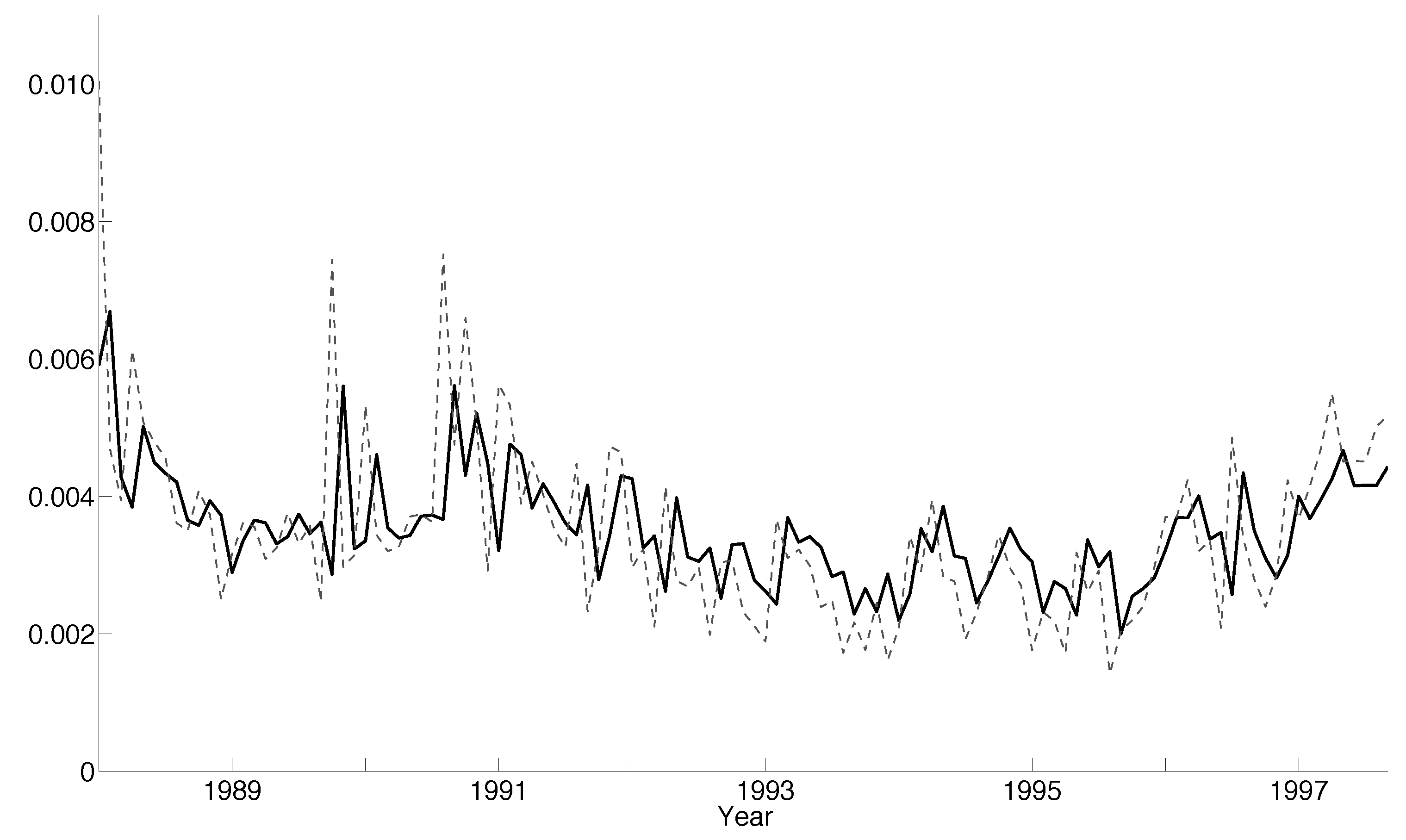
5.4.2. Sample Post the 1987 Crash

To examine the sensitivity of our results with respect to the 1987 crash and the 1997 crash due to the Asian financial crisis, we redo the forecasting exercise so that the first month for which an out-of-sample volatility forecast is obtained is January 1988 and the last month is September 1997.
In Figure 7, we plot the monthly RV and the corresponding one-month-ahead TNTAR forecasts for the out-of-sample period, January 1988-September 1997. As before, forecasts from the TNTAR model captures the overall movements in RV reasonably well. Table 7 reports the forecasting performance of the alternative models under the four forecast accuracy measures. Since the RVs are smaller in this subsample, as expected, the MAE and the MSE are smaller than before. However, the relative performances of the alternative models obtained for the subsample are similar to those obtained for the entire sample, although the HAR and log-HAR models now outperform the ARFIMA models also in MSE. The TNTAR * model once again performs the best overall.

6. Concluding Remarks

In this paper, a simple time series model is introduced to model and forecast RV. The new TNTAR model combines a nonnegative valued process for the error term with the flexibility of Tukey’s power transformation. The transformation is used to improve linearity and reduce heteroskedasticity while the nonnegative support of the error distribution overcomes the truncation problem in the classical Box-Cox setup. The model is semiparametric as the order of m-dependence, support parameter η and functional form of its error term are left unspecified. Consequently, the proposed model is highly parsimonious, having only two parameters that need to be estimated for the purpose of forecasting. A two-stage estimation method is proposed to estimate the parameters of the new model. Simulation studies validate the new estimation method and suggest that it works reasonably well in finite samples.
We empirically examine the forecasting performance of the proposed model relative to a number of existing models, using monthly S&P 500 RV data. The out-of-sample performances were evaluated under four different forecast accuracy measures (MAE, MAPE, MSE and MSPE). We found empirical evidence that our nonnegative model generates highly competitive volatility forecasts.
Why does the simple nonnegative model generate such competitive forecasts? Firstly, as shown in Section 2.2, the logarithmic transformation may not reduce heteroskedasticity and improve normality as well as anticipated. A more general transformation may be required. Secondly, the nonnegative model is highly parsimonious. This new approach is in sharp contrast to the traditional approach which aims to find a model that removes all the dynamics in the original data. When the dynamics are complex, a model with a rich parametrization is called for. This approach may come with the cost of over-fitting and hence may not necessarily lead to superior forecasts. By combining a parametric component for the persistence and a nonparametric error component, our approach presents an effective utilization of more recent information.
Although we only examine the performance of the proposed model for predicting S&P 500 realized volatility one month ahead, the technique itself is quite general and can be applied in many other contexts. First, the method requires no modification when applied to intra-day data to forecast daily RV. In this context, it would be interesting to compare our method to the preferred method in ABDL (2003). Second, our model can easily be extended into a multivariate context by constructing a nonnegative vector autoregressive model. Third, while we focus on stock market volatility in this paper, other financial assets and financial volatility from other financial markets can be treated in the same fashion. Fourth, as two alternative nonnegative models, it would be interesting to compare the performance of our model with that of Cipollini et al. (2006). Finally, it would be interesting to examine the usefulness of the proposed model for multi-step-ahead forecasting. These extensions will be considered in later work.

Author Contributions

All authors contributed equally to all parts of the paper.

Funding

The authors gratefully acknowledge research support from the Jan Wallander and Tom Hedelius Research Foundation (grant P 2006-0166:1), and the Singapore MOE AcRF Tier 2 fund (grant T206B4301-RS) and are thankful to the Sim Kee Boon Institute for Financial Economics at Singapore Management University for partial research support.

Acknowledgments

The authors would like to thank two anonymous referees, Torben Andersen, Federico Bandi, Frank Diebold, Marcelo Medeiros, Bent Nielsen and Neil Shephard for their helpful comments and suggestions. The views expressed in this paper are those of the authors and are not those of J.P. Morgan. All remaining errors are our own.

Conflicts of Interest

The authors declare no conflict of interest.

References

  1. Andersen, Torben G., and Tim Bollerslev. 1998. Answering the skeptics: Yes, standard volatility models do provide accurate forecasts. International Economic Review 39: 885–905. [Google Scholar] [CrossRef]
  2. Andersen, Torben G., Tim Bollerslev, Francis X. Diebold, and Paul Labys. 2001. The distribution of realized exchange rate volatility. Journal of the American Statistical Association 96: 42–55. [Google Scholar] [CrossRef]
  3. Andersen, Torben G., Tim Bollerslev, Francis X. Diebold, and Paul Labys. 2003. Modeling and forecasting realized volatility. Econometrica 71: 579–625. [Google Scholar] [CrossRef]
  4. Barndorff-Nielsen, Ole E., and Neil Shephard. 2001. Non-Gaussian Ornstein-Uhlenbeck-based models and some of their uses in financial economics. Journal of the Royal Statistical Society. Series B (Statistical Methodology) 63: 167–241. [Google Scholar] [CrossRef]
  5. Barndorff-Nielsen, Ole E., and Neil Shephard. 2002. Econometric analysis of realized volatility and its use in estimating stochastic volatility models. Journal of the Royal Statistical Society: Series B (Statistical Methodology) 64: 253–80. [Google Scholar] [CrossRef]
  6. Beran, Jan. 1995. Maximum likelihood estimation of the differencing parameter for invertible short and long memory autoregressive integrated moving average models. Journal of the Royal Statistical Society. Series B (Methodological) 57: 659–72. [Google Scholar] [CrossRef]
  7. Bollerslev, Tim, Ray Y. Chou, and Kenneth F. Kroner. 1992. ARCH modeling in finance: A review of the theory and empirical evidence. Journal of Econometrics 52: 5–59. [Google Scholar] [CrossRef]
  8. Bollerslev, Tim, Robert F. Engle, and Daniel B. Nelson. 1994. Chapter 49 ARCH models. Handbook of Econometrics 4: 2959–3038. [Google Scholar]
  9. Box, George E. P., and David R. Cox. 1964. An analysis of transformations. Journal of the Royal Statistical Society: Series B (Methodological) 26: 211–43. [Google Scholar] [CrossRef]
  10. Chen, Willa W., and Rohit S. Deo. 2004. Power transformations to induce normality and their applications. Journal of the Royal Statistical Society: Series B (Statistical Methodology) 66: 117–30. [Google Scholar] [CrossRef]
  11. Chung, Ching-Fan, and Richard T. Baillie. 1993. Small sample bias in conditional sum-of-squares estimators of fractionally integrated ARMA models. Empirical Economics 18: 791–806. [Google Scholar] [CrossRef]
  12. Cipollini, Fabrizio, Robert F. Engle, and Giampiero M. Gallo. 2006. Vector Multiplicative Error Models: Representation and Inference. Working Paper 12690. Cambridge, UK: National Bureau of Economic Research. [Google Scholar]
  13. Corsi, Fulvio. 2009. A simple approximate long-memory model of realized volatility. Journal of Financial Econometrics 7: 174–96. [Google Scholar] [CrossRef]
  14. Datta, Somnath, and William P. McCormick. 1995. Bootstrap inference for a first-order autoregression with positive innovations. Journal of the American Statistical Association 90: 1289–300. [Google Scholar] [CrossRef]
  15. Davis, Richard A., and William P. McCormick. 1989. Estimation for first-order autoregressive processes with positive or bounded innovations. Stochastic Processes and their Applications 31: 237–50. [Google Scholar] [CrossRef]
  16. Deo, Rohit, Clifford Hurvich, and Yi Lu. 2006. Forecasting realized volatility using a long-memory stochastic volatility model: Estimation, prediction and seasonal adjustment. Journal of Econometrics 131: 29–58. [Google Scholar] [CrossRef]
  17. Diebold, Francis X., and Roberto S. Mariano. 1995. Comparing predictive accuracy. Journal of Business & Economic Statistics 13: 253–63. [Google Scholar]
  18. Doornik, Jurgen A. 2009. An Object-Oriented Matrix Programming Language Ox 6. London: Timberlake Consultants Press. [Google Scholar]
  19. Doornik, Jurgen A., and Marius Ooms. 2004. Inference and forecasting for ARFIMA models with an application to US and UK inflation. Studies in Nonlinear Dynamics & Econometrics 8. [Google Scholar] [CrossRef]
  20. Duan, Jin-Chuan. 1997. Augmented GARCH(p,q) process and its diffusion limit. Journal of Econometrics 79: 97–127. [Google Scholar] [CrossRef]
  21. Feigin, Paul D., and Sidney I. Resnick. 1992. Estimation for autoregressive processes with positive innovations. Communications in Statistics. Stochastic Models 8: 685–717. [Google Scholar] [CrossRef] [Green Version]
  22. Fernandes, Marcelo, and Joachim Grammig. 2006. A family of autoregressive conditional duration models. Journal of Econometrics 130: 1–23. [Google Scholar] [CrossRef] [Green Version]
  23. Ghalanos, Alexios. 2019. Rugarch: Univariate GARCH Models. R Package Version 1.4-1. Available online: https://cran.r-project.org/web/packages/rugarch/index.html (accessed on 4 August 2019).
  24. Ghysels, Eric, Andrew C. Harvey, and Eric Renault. 1996. Stochastic volatility. In Statistical Methods in Finance. Handbook of Statistics. Amsterdam: Elsevier, vol. 14, pp. 119–91. [Google Scholar]
  25. Gonçalves, Sílvia, and Nour Meddahi. 2011. Box-Cox transforms for realized volatility. Journal of Econometrics 160: 129–44. [Google Scholar] [CrossRef]
  26. Granger, Clive W. J., and Paul Newbold. 1976. Forecasting transformed series. Journal of the Royal Statistical Society. Series B (Methodological) 38: 189–203. [Google Scholar] [CrossRef]
  27. Hansen, Peter Reinhard, and Asger Lunde. 2006. Consistent ranking of volatility models. Journal of Econometrics 131: 97–121. [Google Scholar] [CrossRef]
  28. Hansen, Peter Reinhard, Zhuo Huang, and Howard Howan Shek. 2012. Realized GARCH: A joint model for returns and realized measures of volatility. Journal of Applied Econometrics 27: 877–906. [Google Scholar] [CrossRef]
  29. Hentschel, Ludger. 1995. All in the family: Nesting symmetric and asymmetric GARCH models. Journal of Financial Economics 39: 71–104. [Google Scholar] [CrossRef]
  30. Higgins, Matthew L., and Anil K. Bera. 1992. A class of nonlinear ARCH models. International Economic Review 33: 137–58. [Google Scholar] [CrossRef]
  31. Hyndman, Rob J., and Anne B. Koehler. 2006. Another look at measures of forecast accuracy. International Journal of Forecasting 22: 679–88. [Google Scholar] [CrossRef]
  32. Jacod, Jean. 2017. Limit of random measures associated with the increments of a Brownian semimartingale. Journal of Financial Econometrics 16: 526–69. [Google Scholar] [CrossRef]
  33. Jennrich, Robert I. 1969. Asymptotic properties of non-linear least squares estimators. The Annals of Mathematical Statistics 40: 633–43. [Google Scholar] [CrossRef]
  34. J.P. Morgan. 1996. RiskMetricsTM–Technical Document. London: J.P. Morgan. [Google Scholar]
  35. Lopez, Jose A. 2001. Evaluating the predictive accuracy of volatility models. Journal of Forecasting 20: 87–109. [Google Scholar] [CrossRef]
  36. Nielsen, Bent, and Neil Shephard. 2003. Likelihood analysis of a first-order autoregressive model with exponential innovations. Journal of Time Series Analysis 24: 337–44. [Google Scholar] [CrossRef]
  37. Patton, Andrew J. 2011. Volatility forecast comparison using imperfect volatility proxies. Journal of Econometrics 160: 246–56. [Google Scholar] [CrossRef]
  38. Phillips, Peter C.B. 1987. Time series regression with a unit root. Econometrica 55: 277–301. [Google Scholar] [CrossRef]
  39. Poon, Ser-Huang, and Clive W. J. Granger. 2003. Forecasting volatility in financial markets: A review. Journal of Economic Literature 41: 478–539. [Google Scholar] [CrossRef]
  40. Preve, Daniel P. A. 2015. Linear programming-based estimators in nonnegative autoregression. Journal of Banking & Finance 61: 225–34. [Google Scholar]
  41. Shephard, Neil. 2005. Stochastic Volatility: Selected Readings. Oxford: Oxford University Press. [Google Scholar]
  42. Shimotsu, Katsumi, and Peter C. B. Phillips. 2005. Exact local Whittle estimation of fractional integration. The Annals of Statistics 33: 1890–933. [Google Scholar] [CrossRef]
  43. Sowell, Fallaw. 1992. Maximum likelihood estimation of stationary univariate fractionally integrated time series models. Journal of Econometrics 53: 165–88. [Google Scholar] [CrossRef]
  44. Taylor, Stephen J. 2007. Modelling Financial Time Series, 2nd ed. Singapore: World Scientific. [Google Scholar]
  45. Tukey, John W. 1977. Exploratory Data Analysis. Boston: Addison-Wesley. [Google Scholar]
  46. Yu, Jun, Zhenlin Yang, and Xibin Zhang. 2006. A class of nonlinear stochastic volatility models and its implications for pricing currency options. Computational Statistics & Data Analysis 51: 2218–231. [Google Scholar]
1
Generally, the distribution of a Box-Cox transformed random variable cannot be normal as its support is bounded either above or below.
2
See Section 3 for a detailed discussion on the linear programming estimator.
3
In ABDL (2003) RV is referred to as the realized variance, k = 2 N [ p ( t , k ) p ( t , k 1 ) ] 2 . Although the authors build time series models for the realized variance, they forecast the realized volatility. In contrast, the present paper builds time series models for and forecasts, the realized volatility, which seems more appropriate. Consequently, the bias correction, as described in ABDL (2003), is not required.
4
The power parameter is 0.278 which is the estimate of λ in our proposed TNTAR model obtained using the entire S&P 500 monthly RV sample. See Section 3 and Section 5 for further details.
5
Some common m-dependent specifications include u t = ϵ t + ψ ϵ t 1 ( m = 1 ) and u t = ϵ t + ψ ϵ t 1 ϵ t 2 ( m = 2 ), where ϵ t is an i.i.d. sequence of random variables.
6
More generally, suppose that λ = 1 / n for some natural number n, then R V t = φ R V t 1 n + u t n = k = 0 n n k φ n k R V t 1 ( n k ) / n u t k .
7
Whenever necessary we use the subscript T to emphasize on the sample size.
8
For instance, if  y N ( 0 , σ 2 ) and h ( y ) = y 2 then E [ h ( y ) ] = σ 2 h [ E ( y ) ] = 0 .
9
We also applied the exact ML method of Sowell (1992) and the exact local Whittle estimator of Shimotsu and Phillips (2005) in our empirical study and found that the forecasts remained essentially unchanged.
10
The Ox language of Doornik (2009) was used to estimate the two ARFIMA models. Matlab code and data used in this paper can be downloaded from http://www.mysmu.edu/faculty/yujun/research.html.
11
The sGARCH and realGARCH models were estimated using monthly log-returns and the rugarch R package of Ghalanos (2019).
12
While we consider the recursive forecasting scheme one could, of course, also consider the rolling or fixed scheme.
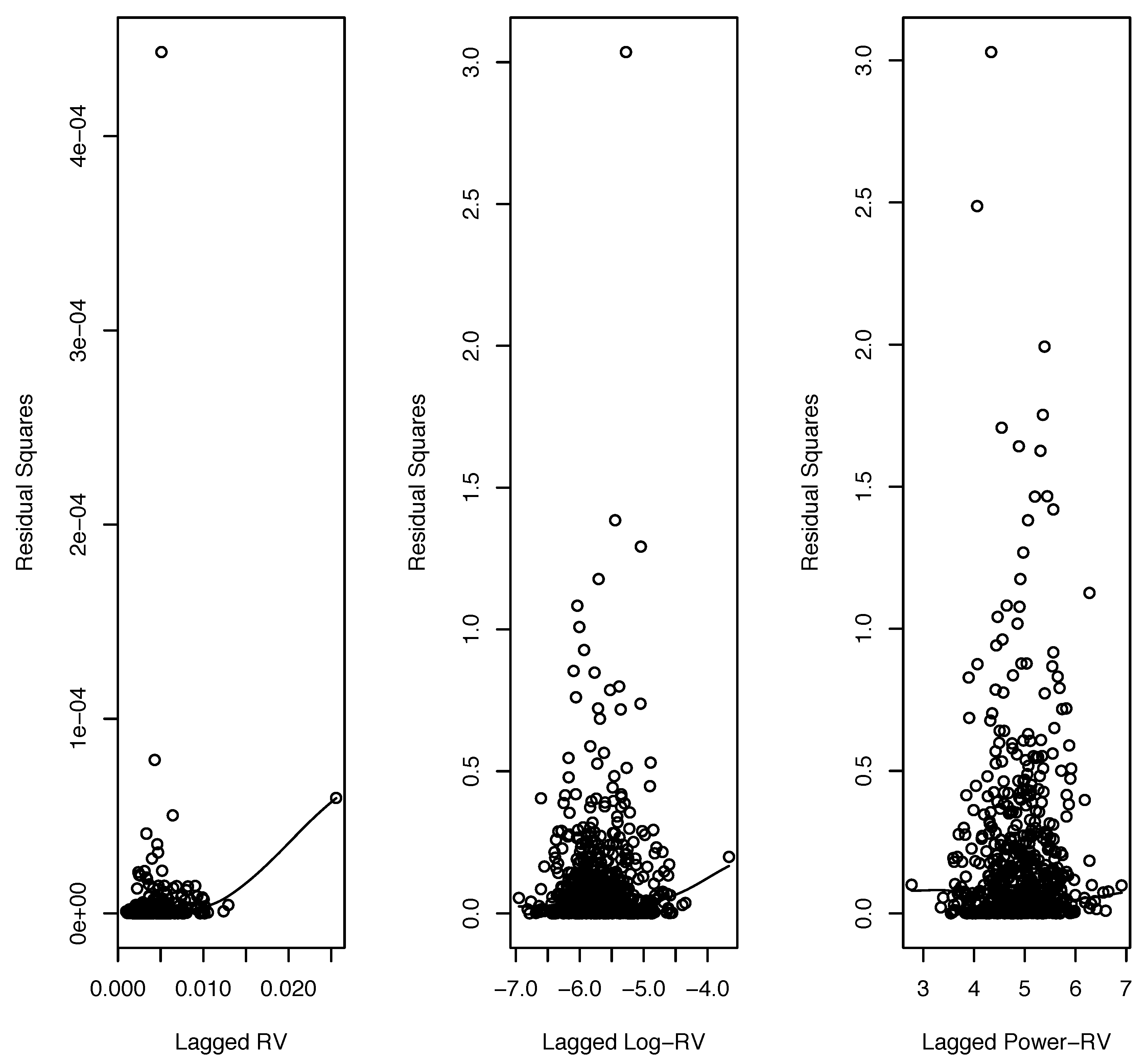
13
We explored all non-zero λ -values on Tukey’s ladder of power transformations in (13) and found that λ = 1 / 2 produced the strongest linear relationship (an increase in R 2 from 0.341 to 0.410).
Figure 1. Plots of squared ordinary least squares (OLS) residuals, obtained from AR(1) regressions for RV, log-RV and power-RV, respectively, against each corresponding explanatory variable. Superimposed are smooth curves fitted using the LOESS method.
Jrfm 12 00139 g001
Figure 2. The top panel displays a time series plot of data simulated from the nonnegative ARMA( 1 , 1 ) process R V t = φ R V t 1 + ϵ t + ψ ϵ t 1 with φ = 0.5 , ψ = 0.75 and i.i.d. standard exponential noise ϵ t . The bottom panel displays the sample paths of the recursive LPEs and OLS estimates for φ in the misspecified AR(1) model R V t = φ R V t 1 + u t , obtained from the sample R V 1 , , R V T for T = 3 , , 100 . The solid line represents the LPEs and the dash-dotted line the OLS estimates.
Jrfm 12 00139 g002
Figure 3. S&P 500 monthly realized volatilities, Jan 1946-Dec 2004. The vertical dashed line indicates the end of the initial sample period used for parameter estimation in our first out-of-sample forecasting exercise.
Jrfm 12 00139 g003
Figure 4. Realized volatility and out-of-sample TNTAR forecasts for the period Jul 1975–Dec 2004. Dashed line: S&P 500 monthly realized volatility. Solid line: one-step-ahead TNTAR forecasts.
Jrfm 12 00139 g004
Figure 5. Recursive TNTAR parameter estimates for the first out-of-sample forecasting exercise. Solid line: path of λ ^ T . Dashed line: path of φ ^ T .
Jrfm 12 00139 g005
Figure 6. The left panel displays a plot of the target variable against the explanatory variable in the AR model (10). The right panel displays a similar plot for the TNTAR model (12), with power transformation parameter λ = 1 / 2 . Superimposed are simple linear regression lines. Data for the period January 1946-June 1975.
Jrfm 12 00139 g006
Figure 7. Realized volatility and out-of-sample TNTAR forecasts for the period Jan 1988–Sep 1997. Dashed line: S&P 500 monthly realized volatility. Solid line: one-month-ahead TNTAR forecasts.
Jrfm 12 00139 g007
Table 1. Summary statistics for S&P 500 monthly RV, log-RV and power-RV over the period Jan 1946–Dec 2004. JB is the p-value of the Jarque-Bera test under the null hypothesis that the data are from a normal distribution.
MeanMedianMaximumSkewnessKurtosisJB
RV 0.004 0.003 0.026 3.307 28.791 0.000
log-RV 5.687 5.726 3.666 0.389 3.657 0.000
power-RV 4.894 4.912 6.908 0.032 3.288 0.259
Table 2. Simulation results for the LPE method. Summary statistics for φ ^ T based on data generated by the nonnegative process R V t 0.25 = φ R V t 1 0.25 + ϵ t + 0.75 ϵ t 1 with i.i.d. standard exponential noise ϵ t . The values of φ considered are 0.25 , 0.50 and 0.75 , respectively. Bias and MSE denotes the empirical bias and mean squared error, respectively. Results based on 100,000 Monte Carlo replications.
T = 200 T = 400 T = 800
ParameterEstimatorBiasMSE BiasMSE BiasMSE
φ = 0.25 φ ^ T 0.047 0.003 0.033 0.001 0.023 0.001
φ = 0.50 φ ^ T 0.028 0.001 0.020 0.001 0.014 0.000
φ = 0.75 φ ^ T 0.013 0.000 0.009 0.000 0.006 0.000
Table 3. Simulation results for the proposed two-stage estimation method. Summary statistics for λ ^ T and φ ^ T based on data generated by the nonnegative process R V t λ = φ R V t 1 λ + ϵ t with i.i.d. standard exponential noise ϵ t . Bias and MSE denotes the empirical bias and mean squared error, respectively. Results based on 100,000 Monte Carlo replications.
T = 200 T = 400 T = 800
ParameterEstimatorBiasMSE BiasMSE BiasMSE
λ = 0.50 λ ^ T 0.197 0.126 0.113 0.069 0.060 0.047
φ = 0.50 φ ^ T 0.106 0.028 0.069 0.018 0.043 0.012
λ = 0.50 λ ^ T 0.139 0.106 0.062 0.067 0.014 0.052
φ = 0.75 φ ^ T 0.064 0.012 0.038 0.006 0.021 0.004
λ = 0.25 λ ^ T 0.195 0.064 0.136 0.033 0.098 0.019
φ = 0.75 φ ^ T 0.144 0.030 0.106 0.017 0.080 0.011
Table 4. Summary statistics for the S&P 500 monthly RV data. JB is the p-value of the Jarque-Bera test under the null hypothesis that the data are from a normal distribution, ρ ^ i is the ith sample autocorrelation.
MeanMaximumSkewnessKurtosisJB ρ ^ 1 ρ ^ 2 ρ ^ 3
RV 0.004 0.026 3.307 28.791 0.000 0.576 0.477 0.408
log-RV 5.687 3.666 0.389 3.657 0.000 0.683 0.595 0.511
Table 5. Forecasting performance of the alternative models under four different accuracy measures. Results based on 354 one-step-ahead forecasts for the period Jul 1975–Dec 2004.
MAE × 10 3 MAPE MSE × 10 6 MSPE
ValueRank ValueRank ValueRank ValueRank
ES1.2689 31.0411 3.86211 15.309
AR0.9756 20.936 3.3129 7.805
HAR0.9452 20.753 3.0185 7.292
log-AR0.9544 20.742 3.0768 7.564
log-HAR0.9371 20.905 2.8663 7.333
sGARCH1.1018 27.239 3.34410 12.437
realGARCH1.0897 28.0510 3.0266 12.938
log-ARFIMA( 0 , d , 0 )0.9615 22.098 2.8471 8.046
log-ARFIMA( 1 , d , 0 )0.9615 22.087 2.8512 8.046
TNTAR0.9544 20.784 3.0757 7.564
TNTAR * 0.9483 20.471 2.9114 6.961
Table 6. p-values of the Diebold-Mariano test for equal predictive accuracy of different models with respect to the benchmark TNTAR model under four different loss functions. Results based on 354 one-step-ahead forecasts for the period Jul 1975–Dec 2004.
MAEMAPEMSEMSPE
ES0.0000.0000.0010.001
AR0.2750.6800.2080.431
HAR0.6600.9610.6070.480
log-AR0.8980.7540.9730.968
log-HAR0.4180.8240.0030.482
sGARCH0.0010.0000.0570.000
realGARCH0.0010.0000.7090.000
log-ARFIMA( 0 , d , 0 )0.7280.0340.0080.188
log-ARFIMA( 1 , d , 0 )0.7250.0350.0080.184
Table 7. Forecasting performance of the alternative models under four different accuracy measures. Results based on 117 one-step-ahead forecasts for the period Jan 1988–Sep 1997.
MAE × 10 3 MAPE MSE × 10 6 MSPE
ValueRank ValueRank ValueRank ValueRank
ES1.07710 35.3811 1.70711 20.1811
AR0.7837 23.888 1.2586 10.738
HAR0.7492 22.683 1.0791 9.282
log-AR0.7796 23.384 1.2728 10.536
log-HAR0.7503 22.452 1.1232 9.373
sGARCH0.9638 32.909 1.3879 18.779
realGARCH0.9919 33.7310 1.48010 19.5110
log-ARFIMA( 0 , d , 0 )0.7796 23.657 1.1603 10.245
log-ARFIMA( 1 , d , 0 )0.7785 23.616 1.1624 10.224
TNTAR0.7774 23.455 1.2607 10.587
TNTAR * 0.7441 21.271 1.1635 8.181

