Article

Multi-Period Investment Strategies under Cumulative Prospect Theory

1
College of Economics and Management, Hunan Normal University, Changsha 410081, China
2
Department of Mathematics and Statistics, McMaster University, 1280 Main Street West, Hamilton, ON L8S 4K1, Canada
*
Author to whom correspondence should be addressed.
These authors contributed equally to this work.
J. Risk Financial Manag. 2019, 12(2), 83; https://doi.org/10.3390/jrfm12020083
Submission received: 10 April 2019 / Revised: 1 May 2019 / Accepted: 5 May 2019 / Published: 11 May 2019
(This article belongs to the Section Mathematics and Finance)

Abstract

:
In this article, inspired by Shi et al., we investigate the optimal portfolio selection with one risk-free asset and one risky asset in a multiple period setting under the cumulative prospect theory (CPT) risk criterion. Compared with their study, our novelty is that we consider a stochastic benchmark and portfolio constraints. By performing a numerical analysis, we test the sensitivity of the optimal CPT investment strategies to different model parameters.

1. Introduction

Expected utility theory (EUT) was a popular decision making model in finance and economics. In reality, however, various decision makers’ behaviour deviates from the implications of expected utility. Substantial experimental and empirical evidence points out that expected utility theory is incompatible with observed human behaviour. The abundant paradoxes lead to the development of a more realistic theory. One of them is prospect theory (PT) (see Tversky and Kahneman 1979). Later, PT was extended to cumulative prospect theory (CPT), since CPT is consistent with the first-order stochastic dominance (see Tversky and Kahneman 1992).
Let us go over some of the literature on CPT. In a continuous-time setting, Jin and Zhou (2008) formulated a general behavioural portfolio selection model under Kahneman and Tversky’s cumulative prospect theory. In a discrete-time setting, Bernard and Ghossoub (2010) considered how a CPT investor chooses his/her optimal portfolio in a single period setting with one risky and one riskless asset. In the same vein, He and Zhou (2011a, 2011b) addressed and formulated the well-posedness of the CPT criterion and investigated the case in which the reference point is different from the risk-free return. The extension to a multi-asset paradigm was done in Pirvu and Schulze (2012) and Kwak and Pirvu (2018). To the best of our knowledge, Carassus and Rasonyi (2015) and Shi et al. (2015) are the only papers to consider the CPT allocation problem in a multi-period framework.
In this paper, we study the optimal portfolio of a CPT investor. Inspired by Shi et al. (2015), we focus on the allocation problem with one risk-free asset and one risky asset in the multiple period setting and with CPT risk criterion. Shi et al. (2015) pointed out that the optimal strategies are time consistent in their setting due to probability distortions. Compared to Shi et al. (2015), one of the contributions of the present article is to allow for time changing benchmark and portfolio constraints. A time changing benchmark is a more realistic model of portfolio management. The work of Strub and Li (2017) investigated weather or not reference point updating led to time-inconsistent investment. They analysed both the time-consistent and time-inconsistent frameworks and concluded that the updating of the reference point non-recursively leads to realistic trading behaviour, which is time inconsistent, and it embeds the disposition effect.
We have to face the time inconsistency of optimal investment strategies in our setting. Due to this predicament, we consider a special type of benchmarking, which renders the optimal strategy time consistent. The optimal strategy is computed by backward induction (see, e.g., Kwak et al. (2014) and Pirvu and Zhang (2013) for similar techniques). Our main result is a recursive formula to characterize the optimal strategies. The stochastic model we consider for the stock return is fairly general. One interesting feature of our recursive formulas characterizing the optimal strategies is that they allow for any distribution specification of stock returns. This is explained by the fact that optimal strategies are computed by backward induction. Our numerical experiments reveal the effect of time on the optimal strategies (this effect cannot be observed in one-period models). The main numerical finding in this regard is that the effect of the model parameters on optimal strategies diminishes slightly as time goes by and it gets closer to maturity.
The remainder of this paper is organized as follows: In Section 2, we present the model. Section 3 outlines the objective, the results and a numerical experiment. The conclusions are presented in Section 4. The paper ends with Appendix A, Appendix B and Appendix C containing the proofs.

2. The Model

We consider a financial market with two investment opportunities: one risk-free asset and one risky asset. The investment horizon is [ 0 , T ] , where T is a finite deterministic positive constant. Let t denote the time of investment, which takes on discrete values ( t = 0 , 1 , , T 1 ) . The future evolution of risky assets’s price is modelled on a probability space ( Ω , F t , F , P ) . The information set at the beginning of period t is F t . Let r t denote the return of the risk-free asset from time t to time t + 1 , and let x t denote the return of the risky asset from time t 1 to time t. We assume that an investor has wealth W t at time t and that he/she invests the amount v t in the risky asset and all of remaining wealth W t v t in the risk-free asset. The investor’s wealth W t + 1 at time t + 1 is given by the self-financing equation:
W t + 1 = ( 1 + r t ) ( W t v t ) + v t ( 1 + x t + 1 ) = ( 1 + r t ) W t + v t ( x t + 1 r t ) = ( 1 + r t ) W t + v t y t + 1 .
Here, y t + 1 is a random variable that represents the dollar excess return on the risky asset over the risk-free asset from time t to time t + 1 . The excess return process { y t } { t = 0 , 1 , , T 1 } , the interest rate process { r t } { t = 0 , 1 , , T 1 } and the amount invested in the risky asset process { v t } { t = 0 , 1 , , T 1 } are adapted stochastic processes, i.e., y t F t , r t F t and v t F t .

2.1. The Benchmarked Wealth

Investors assess the performance of their investments in comparison to a benchmark. This approach is modelled by a benchmark process, which at any point in time divides investment outcomes into gains and losses as follows: a gain occurs whenever the investment outcomes are above the benchmark, and a loss occurs whenever the investment outcomes are below the benchmark.
Let B t , 0 t T , be a positive benchmark process. The benchmarked wealth at time t + 1 , given initial time t, is:
W ¯ t t + 1 = W t t + 1 B t + 1 .
Given the initial time t, the benchmarked wealth at time t + 2 is:
W ¯ t t + 2 = W t t + 2 B t + 2
In general, the benchmarked wealth is given by:
W ¯ t s = W t s B s , s = t + 1 , t + 2 , , T .

Examples of the Benchmark

One benchmark process is the constant throughout time benchmark B , where B is a constant. This kind of benchmark is considered in Shi et al. (2015). Another benchmark process is obtained by investing the initial/current wealth in the risk-free asset. Other examples of benchmarks are an index of stochastic assets and the expected wealth (for more on this, see Pirvu and Schulze 2012).

2.2. Portfolio Constraints

It is often the case that managers impose risk limits on the trading strategies. The risk control mechanism has two components: one internal (imposed by risk management departments) and one external (accredited regulatory institutions). Thus, it is only natural to consider portfolio constraints. In the following, we introduce the class of admissible strategies.
Definition 1.
The set of admissible strategies at time t is A t ,
A t = { v t F t | A | W t | v t B | W t | }
for some constants A 0 < B .
This formal definition is saying that the investments in the risky asset are acceptable if the corresponding portfolio proportion invested in the risky asset is bounded.
The fact that A 0 is saying that short selling is allowed in this market. In practice, there are rules about short selling; for the special case of Chinese financial markets: “The underlying stocks for short selling should have more than 200 million shares or the market value in circulation should have more than 800 million RMB; the number of shareholders should be more than 4000,” page 263 in Gregoriou (2011).
The portfolio constraint A | W t | v t sets a (negative) floor on the portfolio proportion invested in the risky asset, which is the same as limiting the short selling amount (some portfolio managers tend to do that). On the other hand, the constraint v t B | W t | limits the exposure to the risky asset, which is in line with the industry practice: “In 1991, the National Association of Insurance Commissioners (NAIC) imposed higher reserve requirements on insurance companies holdings of junk bonds, specifying a 20% cap on the assets insurers may hold in junk bonds. Many pension funds place limits on the fraction of a portfolio that can be invested in junk bonds,” Da and Gao (2009) (junk bonds are a special type of risky assets that have a high return, but also posses a high risk). Other types of portfolio constraints are: bound constraints on specific assets, cardinality constraints, and turnover constraints, just to mention a few (see Guijarro (2018) for more on cardinality constraints). We also point the interested reader to Garcia et al. (2018).

2.3. The CPT Risk Criterion

The investor gets utility from gains and disutility from losses. The benchmark differentiates gains from losses. Let us introduce the following formal definitions.
Definition 2
(See Tversky and Kahneman 1979, 1992). The value function u is defined as follows:
u ( x ) = u + ( x ) i f x 0 , u ( x ) i f x < 0 ,
where u + : R ¯ + R ¯ + and u : R ¯ + R ¯ + satisfy:
(i) 
u ( 0 ) = u + ( 0 ) = u ( 0 ) = 0 ;
(ii) 
u + ( + ) = u ( + ) = + ;
(iii) 
u + ( x ) = x α , with 0 < α < 1 and x 0 ;
(iv) 
u ( x ) = λ x α with λ > 1 and x 0 .
It is important to point out that the CPT objective considers deviation from the benchmark, so the argument x in the utility function u ( x ) is not a wealth level, but a deviation of wealth from the benchmark.
Definition 3.
Let F X ( · ) be the cumulative distribution function (CDF) of a random variable X. The probability distortions are denoted by T + and T . We define the two probability weight functions (distortions) T + : [ 0 , 1 ] [ 0 , 1 ] and T : [ 0 , 1 ] [ 0 , 1 ] as follows:
T + ( F X ( x ) ) = F X γ ( x ) ( F X γ ( x ) + ( 1 F X ( x ) ) γ ) 1 / γ , w i t h 0.28 < γ < 1 , T ( F X ( x ) ) = F X δ ( x ) ( F X δ ( x ) + ( 1 F X ( x ) ) δ ) 1 / δ , w i t h 0.28 < δ < 1 .
The choice of γ , δ > 0.28 guarantees that T + , T are increasing Ingersoll (2008).
Definition 4.
Define the objective function of the CPT investor, denoted by U ( W ) , as:
U ( W ) = 0 + T + ( 1 F W ( x ) ) d u + ( x ) 0 + T ( F W ( x ) ) d u ( x ) ,
where W is the benchmarked wealth. U ( W ) is a sum of two Choguet integrals (see Choquet 1953 and Chateauneuf et al. 2000). It is well-defined when:
α < 2 min ( δ , γ ) ,
(see Proposition 2 in Pirvu and Schulze (2012)).
From Definition 4, it follows that an objective function of the CPT investor at time t is:
U ( W ¯ t T ) = 0 + T + ( 1 F W ¯ t T ( x ) ) d u + ( x ) 0 + T ( F W ¯ t T ( x ) ) d u ( x ) .
As we mention in Section 3.3, this risk criterion is time inconsistent; thus, we propose a special case of benchmarked wealth; that is, perform benchmarking at time T 1 only1. Thus, if the initial time is t ( t = 0 , 1 , 2 , , T 1 ), then the benchmarked wealth at T is:
W ̲ t T = v T 1 y T given that the initial time is t .
The objective function is then defined as follows:
U ( W ̲ T 1 T ) = 0 + T + ( 1 F W ̲ T 1 T ( x ) ) d u + ( x ) 0 + T ( F W ̲ T 1 T ( x ) ) d u ( x ) ,
and:
U ( W ̲ t T ) = E [ U ( W ̲ T 1 T ) | F t ] .
The above equation naturally extends U ( W ̲ T 1 T ) at earlier times, and this makes sense in light of (8).

3. Methodology

Let us begin with formulating the CPT investor objective. In a first step, we consider the one-period model.

3.1. Single Period Objective

We assume that the current time is T 1 . Recall that the benchmarked wealth at time T is:
W ̲ T 1 T = v T 1 y T .
The CPT investor objective is to find the portfolio that leads to the highest possible prospect value; consequently, the investor solves the following portfolio problem:
( P ) max v T 1 A T 1 U ( W ̲ T 1 T ) = max v T 1 A T 1 0 + T + ( 1 F W ̲ T 1 T ( x ) ) d u + ( x ) 0 + T ( F W ̲ T 1 T ( x ) ) d u ( x ) .
The portfolio yielding the highest possible prospect value, i.e., the optimal portfolio, is v T 1 * given by:
v T 1 * = a r g max v T 1 A T 1 U ( W ̲ T 1 T ) = a r g max v T 1 A T 1 0 + T + ( 1 F W ̲ T 1 T ( x ) ) d u + ( x ) 0 + T ( F W ̲ T 1 T ( x ) ) d u ( x ) .

3.2. Multiple Period Objective

Let us consider a multiple period model. In order to get a time-consistent optimal strategy, we work with the benchmarked wealth W ̲ t T , defined in (8). The CPT investor objective is to solve the following portfolio problem:
( P ) max v i A i , i = t , t + 1 , T 1 U ( W ̲ t T ) = max v i A i , i = t , t + 1 , T 1 E 0 + T + ( 1 F W ̲ T 1 T ( x ) ) d u + ( x ) 0 + T ( F W ̲ T 1 T ( x ) ) d u ( x ) | F t .
Having stated the objectives, let us turn to the issue of time inconsistency.

3.3. Time Inconsistency

As already pointed out in Shi et al. (2015), the optimal strategy is time inconsistent due to the nonlinear distortions. That is, the optimal strategy computed in the past is not implemented unless there is a commitment mechanism. Let us define v T 1 * the time T 1 portfolio and ( v ^ T 2 , v ^ T 1 ) the time T 2 optimal portfolio:
v T 1 * = a r g max v T 1 A T 1 U ( W ̲ T 1 T ) ,
and
( v ^ T 2 , v ^ T 1 ) = a r g max v T 2 A T 2 , v T 1 A T 1 U ( W ̲ T 2 T ) .
It turns out that v T 1 * v ^ T 1 , which means that the investor is time inconsistent, i.e., the time T 2 optimal portfolio is not implemented at time T 1 when another portfolio is optimal.

3.4. Results

After formulating the objective, we are ready to present our results. Our exposition starts with the single period case. We manage to analyse the investor portfolio optimization problem in terms of the wealth being positive/negative. The result is summarized in the following proposition.
Proposition 1.
The optimal prospect value is:
max v T 1 A T 1 U ( W ̲ T 1 T ) = W T 1 α A T 1 I W T 1 0 ( W T 1 ) α B T 1 I W T 1 < 0 ,
where:
A T 1 = max z [ A , B ] g T 1 ( z ) ,
B T 1 = max z [ B , A ] l T 1 ( z ) ,
g T 1 ( z ) = z α k ( T 1 ) I z [ 0 , B ] + ( z ) α h ( T 1 ) I z [ A , 0 ]
l T 1 ( z ) = ( z ) α k ( T 1 ) I z [ B , 0 ] + z α h ( T 1 ) I z [ 0 , A ]
k ( T 1 ) = 0 + T + ( 1 F y T ( x ) ) d u + ( x ) 0 + T ( F y T ( x ) ) d u ( x )
and:
h ( T 1 ) = 0 + T + ( 1 F y T ( x ) ) d u + ( x ) 0 + T ( F y T ( x ) ) d u ( x )
Proof. 
The proof is given in Appendix A. □
Theorem 1.
The optimal CPT investment strategy is:
v T 1 * = k T 1 * W T 1 i f W T 1 0 , k ^ T 1 * W T 1 i f W T 1 < 0 ,
where:
k T 1 * = a r g max z [ A , B ] g T 1 ( z ) , k ^ T 1 * = a r g max z [ B , A ] l T 1 ( z ) .
Proof. 
The above conclusion is derived from Proposition 1. □
Subsequently, we consider the optimal strategies in the multiple periods. In order to ease the exposition, we present the two-period model case; when the initial time is T 2 , the following result is established.
Proposition 2.
The maximum CPT value is given recursively by:
max v T 2 A T 2 , v T 1 A T 1 U ( W ̲ T 2 T ) = A T 2 W T 2 α I W T 2 0 B T 2 ( W T 2 ) α I W T 2 < 0 ,
where:
A T 2 = max z [ A , B ] g T 2 ( z ) ,
B T 2 = max z [ B , A ] l T 2 ( z ) ,
g T 2 ( z ) = E [ A T 1 ( 1 + r T 2 + y T 1 z ) α I { 1 + r T 2 + y T 1 z 0 } B T 1 ( 1 r T 2 y T 1 z ) α I { 1 + r T 2 + y T 1 z < 0 } | F T 2 ]
l T 2 ( z ) = E [ A T 1 ( 1 r T 2 y T 1 z ) α I { 1 + r T 2 + y T 1 z < 0 } B T 1 ( 1 + r T 2 + y T 1 z ) α I { 1 + r T 2 + y T 1 z 0 } | F T 2 ] .
and A T 1 , B T 1 are given by (16), (17).
Proof. 
The proof is done in Appendix B. □
As a consequence of this, we can obtain the following key proposition and theorem for multiple periods. They provide an algorithm to compute iteratively backward (starting from the last time period [ T 1 , T ] and then going to [ T 2 , T ] , etc.) the optimal prospect value and the corresponding optimal portfolio.
Proposition 3.
Given the initial time t , the optimal CPT value is given recursively by:
max v i A i , i = t , t + 1 , T 1 U ( W ̲ t T ) = A t W t α I W t 0 B t ( W t ) α I W t < 0 ,
where:
A t = max z [ A , B ] g t ( z ) ,
B t = max z [ B , A ] l t ( z ) ,
g t ( z ) = E [ A t + 1 ( 1 + r t + y t + 1 z ) α I { 1 + r t + y t + 1 z 0 } B t + 1 ( 1 r t y t + 1 z ) α I { 1 + r t + y t + 1 z < 0 } | F t ]
l t ( z ) = E [ A t + 1 ( 1 r t y t + 1 z ) α I { 1 + r t + y t + 1 z < 0 } B t + 1 ( 1 + r t + y t + 1 z ) α I { 1 + r t + y t + 1 z 0 } | F t ] ,
A T 1 , B T 1 are given by (16), (17), A T 2 , B T 2 are given by (19), (20), etc.
Proof. 
We prove this in Appendix C. □
The following theorem is our main result of the paper.
Theorem 2.
The optimal CPT investment strategy ( v 0 * , v 1 * , , v T * ) is given recursively for t = T 1 , T 2 , , 0 by:
v t * = k t * W t i f W t 0 , k ^ t * W t i f W t < 0 ,
k t * = a r g max z [ A , B ] g t ( z )
and:
k ^ t * = a r g max z [ B , A ] l t ( z ) .
Proof. 
The above result is derived from Proposition 3. □

3.5. Numerical Simulation

We assumed that the excess return y t follows a normal distribution N ( μ , σ ) . The interest rate was set to follow the Ho and Lee model (see Ishimura et al. 2013):
r t = 0.03 + 0.003 t Z , Z N ( 0 , 1 ) .
This choice of modelling the excess return and the interest rate was to make the model tractable. The S-shaped utility, the probability distortions and especially the multiple periods increase the computational complexity.
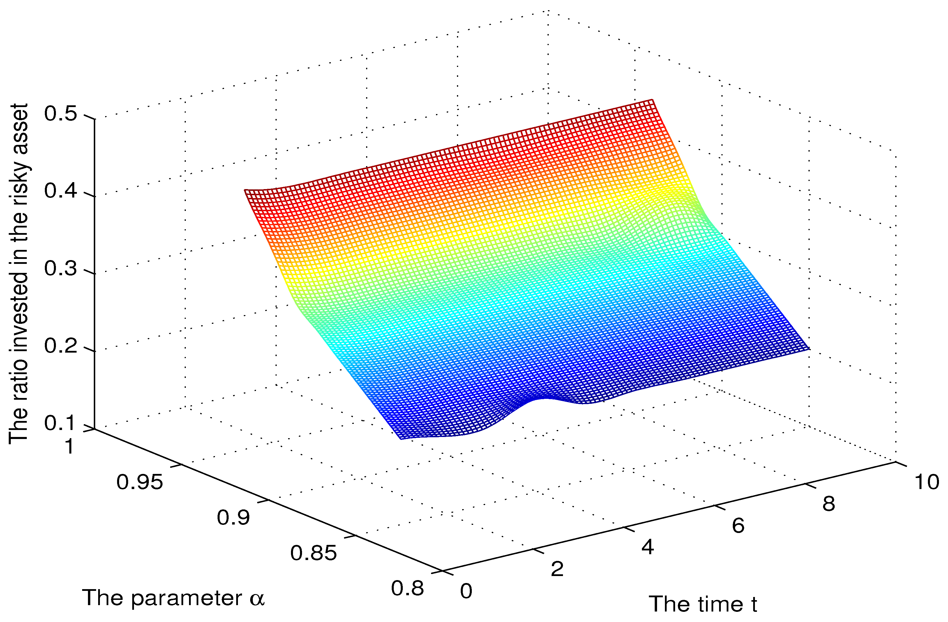
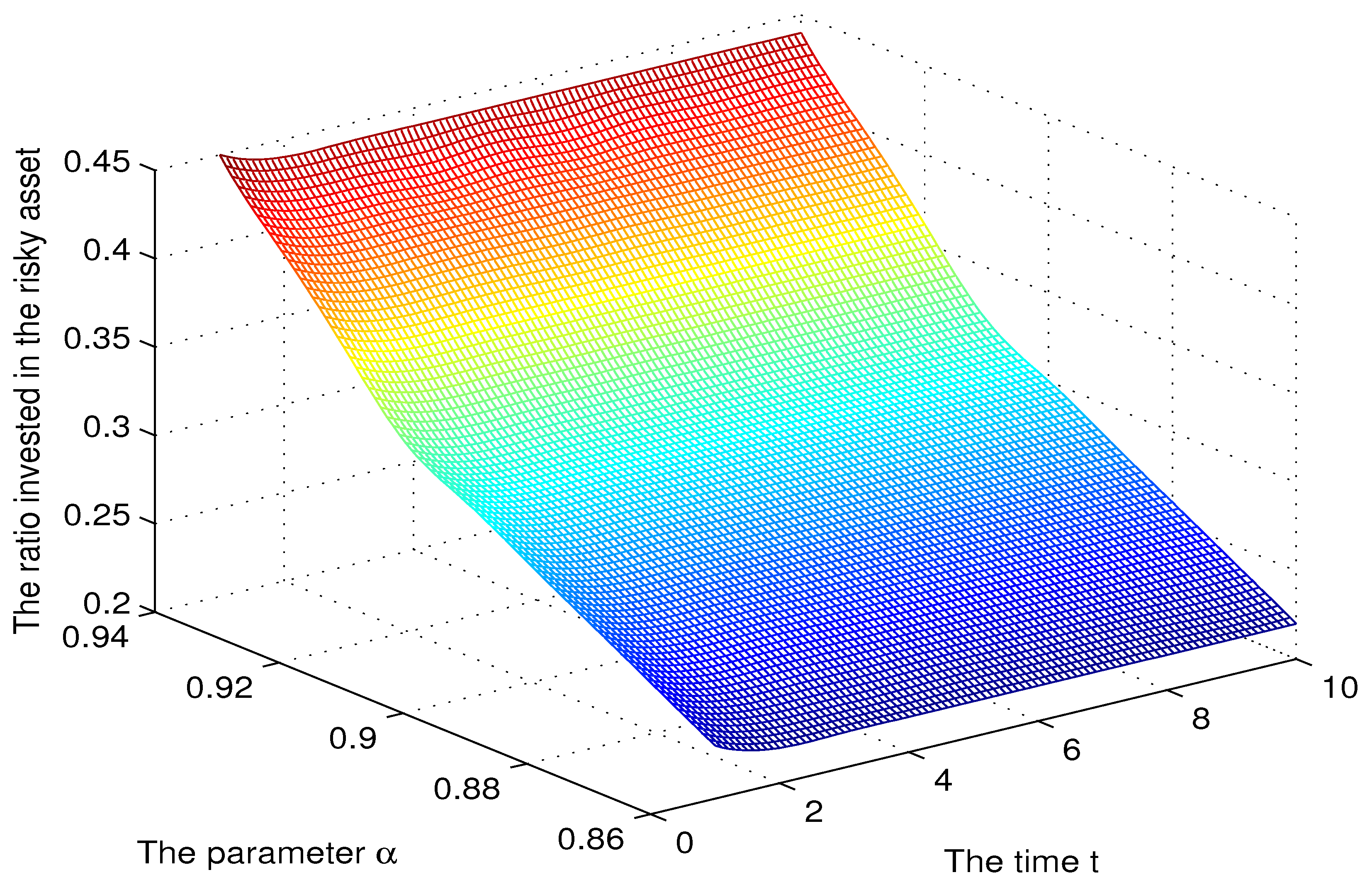
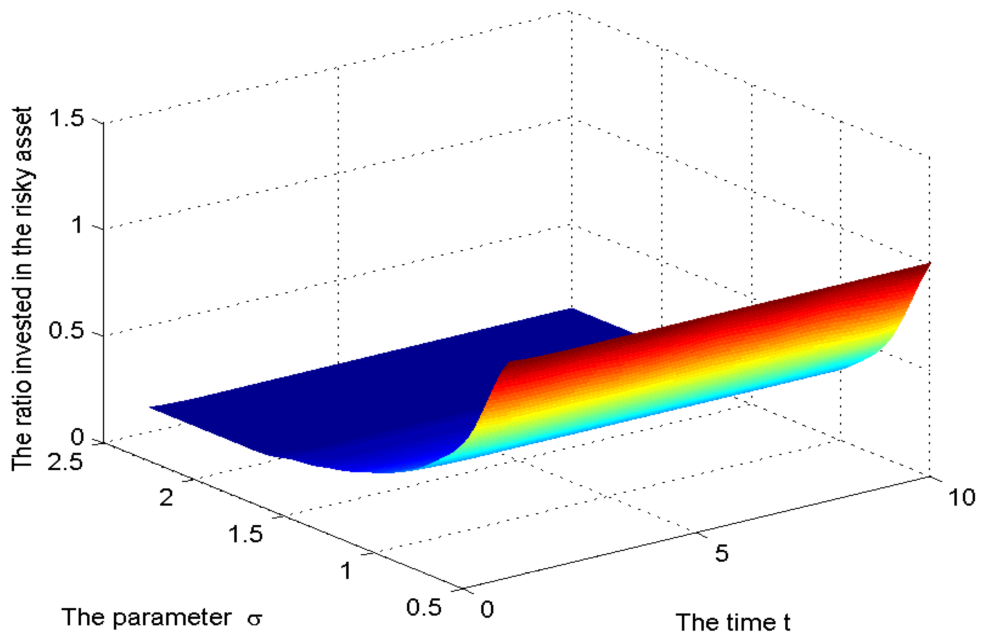
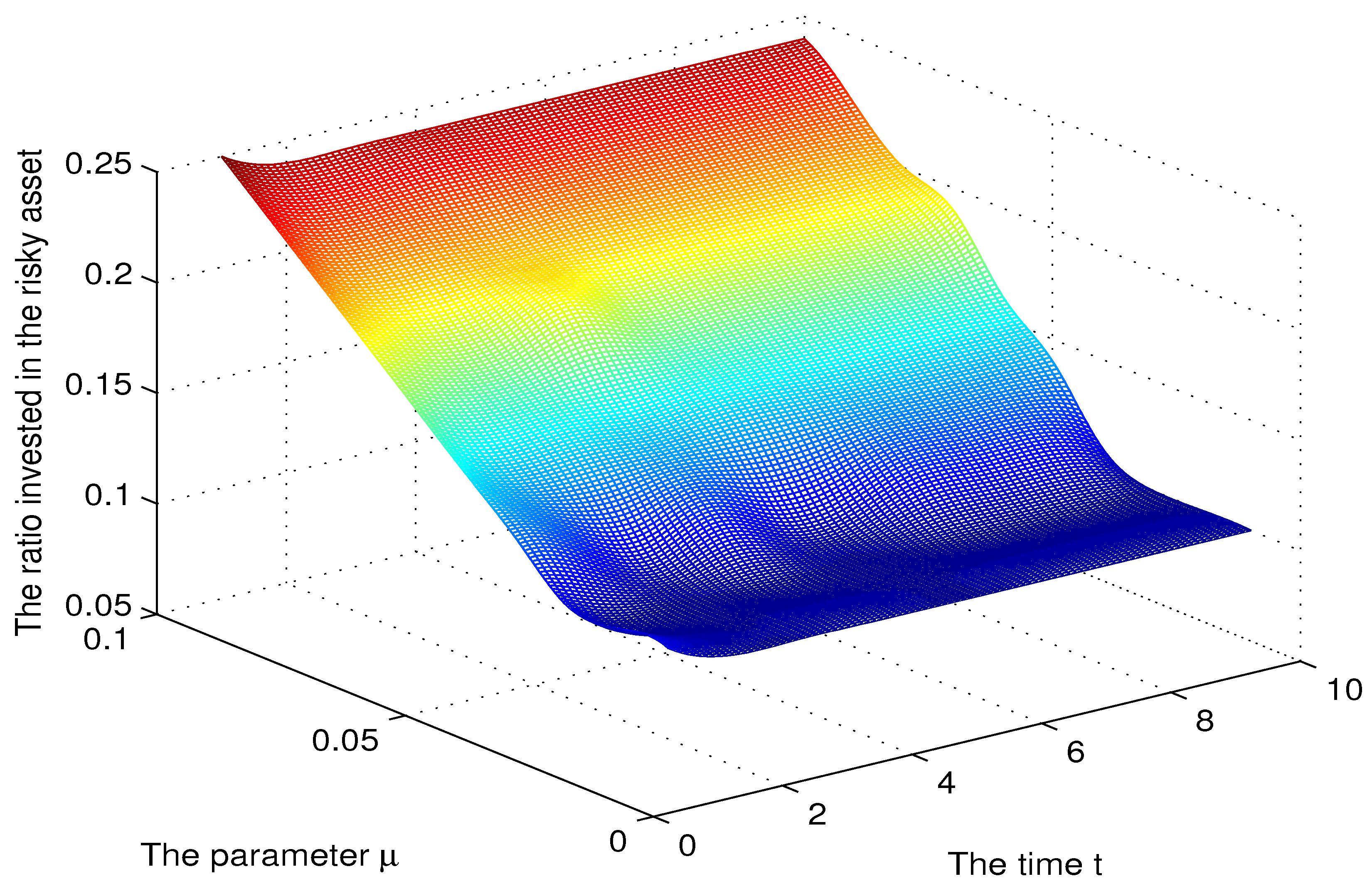
Let the risk limits be A = 5 , B = 5 . We tested the sensitivity of the optimal solution to different parameters α , μ and δ . Moreover, we analysed how CPT investors’ psychology and the characteristics of the stock influence the optimal CPT investment strategies. When we tested sensitivity, we set W 0 = 0.8 and discussed the sensitivity of the t th period (t = 0, 1, …, 10). Following Tversky and Kahneman (1992), we set λ = 2.25 , γ = 0.61 , and δ = 0.69 . Let μ = 0.045 , σ = 1.69 in Figure 1 and Figure 2 and α = 0.88 in Figure 3 and Figure 4 (this choice is taken from Tversky and Kahneman (1992)).
In order to reveal the effect of CPT investors’ psychology on the optimal portfolio choice, we analysed the sensitivity of the optimal solution to the parameter α (see Figure 1 and Figure 2). The ratio of wealth invested in the risky asset was increasing in α . This trend was also observed in Pirvu and Schulze (2012), and it is explained by an increased risk appetite produced by a higher α . Indeed, 1 α is the Arrow–Pratt measure of relative risk aversion (RRA) or the coefficient of relative risk aversion, so higher α means less risk aversion. We see from Figure 2 that a 10 % decrease in α led to a 50 % decrease in the ratio invested in the risky asset. For high values of α , the ratio invested in the risky asset was slowly decreasing in time.
As expected, the investment in the risky asset was decreasing in σ since a higher σ makes the risky asset a less attractive investment opportunity. The effect of σ on the ratio invested in the risky asset is more pronounced for higher values of σ , a fact explained by the CPT agent being conservative. The investment in the risky asset was increasing in μ , and this is justified since a higher μ makes the risky asset more attractive. We see from Figure 4 that as μ increased from 5– 10 % , the ratio increased from 10– 25 % .
Let us have a closer look at the time variability of the ratio of wealth invested in the risky asset we see in these plots. There are two points to make here: (1) there was not much variation over time of this ratio (a similar phenomenon can be observed in Example 2, page 403, in Li and Ng (2000)); (2) the ratio was slowly decreasing in time; and this monotonicity is explained by the fact that the CPT agent becomes more conservative as the time to maturity comes closer, and there is less time to adjust the trade.

4. Conclusions

This paper studied the optimal portfolio problem of a CPT investor in the multiple period setting with one risk-free asset and one risky asset. The risk free return was stochastic, and constraints were imposed on the trading portfolios. The optimal strategies were time consistent in this paradigm due to probability distortions. In order to get around this problem, we imposed a special portfolio benchmarking, which made the optimal strategy time consistent. Our main result was a recursive formula, which led to the optimal portfolio strategies.
A numerical experiment revealed the effect of CPT investors’ psychology on the optimal portfolio choice. We found out that, as expected, the ratio of wealth invested in the risky asset was decreasing when the coefficient of relative risk aversion increased. Moreover, as expected, the investment in the risky asset was decreasing in the risky asset volatility and increasing in the risky asset return. The effect of the model parameters on optimal strategies was slightly diminishing as time went by.
The recursive formula yielding the optimal portfolios was general, and it did not depend on the distribution of the risky asset. However, in our numerical experiment, because of computational tractability issues, we assumed that the risky asset’s return was normally distributed, which is a quite restrictive assumption. The choice of other return distributions, not necessarily symmetric, such as the Student t-distribution, we leave as a topic of future research. Another limitation of our work was the special type of benchmarking proposed. This was done to overcome the difficulties caused by the time inconsistency (due to the nonlinear portfolio distortions). A future research direction is to investigate this portfolio allocation problem under other types of benchmarking as well.

Author Contributions

All authors made substantial contribution to this paper.

Funding

This research was funded by the Humanities and Social Science Project of the Ministry of Education (No. 17YJC790020) and NSERC Grant 396-5058-14. This funding did not lead to any conflicts of interest regarding the publication of this manuscript.

Conflicts of Interest

The authors declare no conflict of interest.

Appendix A. Proof of Proposition 1

Proof. 
When W T 1 0 and 0 v T 1 B W T 1 , we directly employ the result of Bernard and Ghossoub (2010) in order to get:
U ( W ̲ T 1 T ) = v T 1 α 0 + T + ( 1 F y T ( x ) ) d u + ( x ) 0 + T ( F y T ( x ) ) d u ( x ) .
Let v T 1 = W T 1 z , so:
U ( W ̲ T 1 T ) = W T 1 α z α 0 + T + ( 1 F y T ( x ) ) d u + ( x ) 0 + T ( F y T ( x ) ) d u ( x ) . = W T 1 α z α k ( T 1 )
Similarly, when W T 1 0 and A W T 1 v T 1 0 , we can show that:
U ( W ̲ T 1 T ) = ( v T 1 ) α 0 + T + ( 1 F y T ( x ) ) d u + ( x ) 0 + T ( F y T ( x ) ) d u ( x ) = W T 1 α ( z ) α 0 + T + ( 1 F y T ( x ) ) d u + ( x ) 0 + T ( F y T ( x ) ) d u ( x ) = W T 1 α ( z ) α h ( T 1 ) .
Hence, when W T 1 0 , we have that:
U ( W ̲ T 1 T ) = W T 1 α [ z α k ( T 1 ) I z [ 0 , B ] + ( z ) α h ( T 1 ) I z [ A , 0 ] ] = W T 1 α g T 1 ( z ) .
When W T 1 < 0 and 0 v T 1 B W T 1 , one easily gets:
U ( W ̲ T 1 T ) = ( W T 1 ) α ( z ) α 0 + T + ( 1 F y T ( x ) ) d u + ( x ) 0 + T ( F y T ( x ) ) d u ( x ) = ( W T 1 ) α ( z ) α k ( T 1 )
When W T 1 < 0 and A W T 1 v T 1 0 , we show that:
U ( W ̲ T 1 T ) = ( v T 1 ) α 0 + T + ( 1 F y T ( x ) ) d u + ( x ) 0 + T ( F y T ( x ) ) d u ( x ) = ( W T 1 ) α z α 0 + T + ( 1 F y T ( x ) ) d u + ( x ) 0 + T ( F y T ( x ) ) d u ( x ) = ( W T 1 ) α z α h ( T 1 ) .
Therefore, when W T 1 < 0 , we have that:
U ( W ̲ T 1 T ) = ( W T 1 ) α [ ( z ) α k ( T 1 ) I z [ B , 0 ] + z α h ( T 1 ) I z [ 0 , A ] ] = ( W T 1 ) α l T 1 ( z ) .
 □

Appendix B. Proof of Proposition 2

Proof. 
Since:
W ̲ T 2 T = v T 1 y T given that the initial time is T 2 ,
and:
U ( W ̲ T 2 T ) = E [ U ( W ̲ T 1 T ) | F T 2 ] ,
then:
max v T 2 A T 2 , v T 1 A T 1 U ( W ̲ T 2 T ) = max v T 2 A T 2 E [ max v T 1 A T 1 U ( W ̲ T 1 T ) | F T 2 ] .
By applying Proposition 1 to the above equation, one gets:
max v T 2 A T 2 , v T 1 A T 1 U ( W ̲ T 2 T ) = max v T 2 A T 2 E [ W T 1 α A T 1 I W T 1 0 ( W T 1 ) α B T 1 I W T 1 < 0 | F T 2 ] .
From Equation (1), it follows that:
W T 1 = ( 1 + r T 2 ) W T 2 + v T 2 y T 1 .
Let
v T 2 = W T 2 k T 2 .
When W T 2 0 , it is straightforward to show that:
max v T 2 A T 2 , v T 1 A T 1 U ( W ̲ T 2 T ) = W T 2 α max k T 2 [ A , B ] E [ ( 1 + r T 2 + k T 2 y T 1 ) α A T 1 I 1 + r T 2 + k T 2 y T 1 0 ( 1 r T 2 k T 2 y T 1 ) α B T 1 I 1 + r T 2 + k T 2 y T 1 < 0 | F T 2 ] = W T 2 α max k T 2 [ A , B ] g T 2 ( k T 2 ) = W T 2 α A T 2 .
When W T 2 < 0 , similarly, we confirm that:
U ( W ̲ T 2 T ) = ( W T 2 ) α max k ^ T 2 [ B , A ] E [ ( 1 r T 2 k ^ T 2 y T 1 ) α A T 1 I 1 + r T 2 + k ^ T 2 y T 1 < 0 ( 1 + r T 2 + k ^ T 2 y T 1 ) α B T 1 I 1 + r T 2 + k ^ T 2 y T 1 0 | F T 2 ] = ( W T 2 ) α max k ^ T 2 [ B , A ] l T 2 ( k ^ T 2 ) = ( W T 2 ) α B T 2 .
Therefore, Proposition 2 holds. □

Appendix C. Proof of Proposition 3

Proof. 
We use mathematical induction to prove this proposition. Propositions 1 and 2 display that the conclusion of Proposition 3 holds at times T − 1 and T − 2. We suppose the conclusion holds at time t + 1 . Namely,
max v i A i , i = t + 1 , t + 2 T 1 U ( W ̲ t + 1 T ) = A t + 1 W t + 1 α I W t + 1 0 B t + 1 ( W t + 1 ) α I W t + 1 < 0 .
Since:
W ̲ t T = v T 1 y T given that the initial time is t ,
and:
U ( W ̲ t T ) = E [ U ( W ̲ T 1 T ) | F t ] ,
then:
max v i A i , i = t , t + 1 T 1 U ( W ̲ t T ) = max v t A t E t [ max v i A i , i = t , t + 1 T 1 U ( W ̲ t + 1 T ) ] = max v t A t E [ A t + 1 W t + 1 α I W t + 1 0 B t + 1 ( W t + 1 ) α I W t + 1 < 0 | F t ] .
Let
v t = W t k t .
Since:
W t + 1 = ( 1 + r t ) W t + v t y t + 1 ,
we have:
W t + 1 = W t ( 1 + r t + k t y t + 1 ) .
Therefore, when W t 0 ,
max v i A i , i = t , t + 1 T 1 U ( W ̲ t T ) = W t α max k t [ A , B ] E [ ( 1 + r t + k t y t + 1 ) α A t + 1 I 1 + r t + k t y t + 1 0 ( 1 r t k t y t + 1 ) α B t + 1 I 1 + r t + k t y t + 1 < 0 | F t ] = W t α max k t [ A , B ] g t ( k t ) = W t α A t .
When W t < 0 , we can similarly find that:
max v i A i , i = t , t + 1 T 1 U ( W ̲ t T ) = ( W t ) α max k ^ t [ B , A ] E [ ( 1 r t k ^ t y t + 1 ) α A t + 1 I 1 + r t + k ^ t y t + 1 < 0 ( 1 + r t + k ^ t 2 y t + 1 ) α B t + 1 I 1 + r t + k ^ t y t + 1 0 | F t ] = ( W t ) α max k ^ t [ B , A ] l t ( k ^ t ) = ( W t ) α B t .
Thus, Proposition 3 holds. □

References

  1. Bernard, Carole, and Mario Ghossoub. 2010. Static Portfolio Choice under Cumulative Prospect Theory. Mathematics and Financial Economics 2: 277–306. [Google Scholar] [CrossRef]
  2. Carassus, Laurence, and Miklos Rasonyi. 2015. On optimal investment for a behavioural investor in multi-period incomplete market models. Math. Finance 25: 115–53. [Google Scholar] [CrossRef]
  3. Chateauneuf, Alain, Rose-Anne Dana, and Jean-Marc Tallon. 2000. Optimal risk-sharing rules and equilibria with Choquet-expected-utility. Journal of Mathematical Economics 34: 191–214. [Google Scholar] [CrossRef] [Green Version]
  4. Choquet, Gustave. 1953. Theory of capacities. Annales de l’Institut Fourier 5: 131–295. [Google Scholar] [CrossRef]
  5. Da, Zhi, and Pengjie Gao. 2009. Clientele Change, Persistent Liquidity Shock, and Bond Return Reversals after Rating Downgrades. SSRN. [Google Scholar] [CrossRef]
  6. Garcia, Fernando, Francisco Guijarro, Javier Oliver, and Rima Tamosiuniene. 2018. Hybrid fuzzy neural network to predict price direction in the German DAX-30 index. Technological and Economic Development of Economy 24: 2161–78. [Google Scholar] [CrossRef]
  7. Gregoriou, Greg N. 2011. Handbook of Short Selling, 1st ed.Waltham: Academic Press, eBook ISBN 9780123877253, Hardcover ISBN 9780123877246. [Google Scholar]
  8. Guijarro, Francisco. 2018. A similarity measure for the cardinality constrained frontier in the mean–variance optimization model. Journal of the Operational Research Society 69: 928–45. [Google Scholar] [CrossRef]
  9. He, Xue Dong, and Xun Yu Zhou. 2011a. Portfolio Choice under Cumulative Prospect Theory: An Analytical Treatment. Management Science 57: 315–31. [Google Scholar] [CrossRef]
  10. He, Xue Dong, and Xun Yu Zhou. 2011b. Portfolio Choice via Quantiles. Mathematical Finance 21: 203–31. [Google Scholar] [CrossRef]
  11. Ingersoll, Jonathan. 2008. Non-monotonicity of the Tversky Kahneman probability-weighting function: A cautionary note. European Financial Management 14: 385–90. [Google Scholar] [CrossRef]
  12. Ishimura, Naoyuki, Bold Javkhlan, MasaAki Nakamura, and Zheng Wei. 2013. Models of the Short Interest Rate in Discrete Processes. Open Journal of Applied Sciences 3: 12–14. [Google Scholar] [CrossRef]
  13. Jin, Hanqing, and Xun Yu Zhou. 2008. Behavioral portfolio selection in continuous time. Mathematical Finance 18: 385–426. [Google Scholar] [CrossRef]
  14. Kwak, Minsuk, and Traian A. Pirvu. 2018. Cumulative Prospect Theory with Skewed Return Distribution. SIAM Journal on Financial Mathematics 9: 54–89. [Google Scholar] [CrossRef]
  15. Kwak, Minsuk, Traian A. Pirvu, and Huayue Zhang. 2014. A multi-period equilibrium pricing model. Journal of Applied Mathematics 2014: 408685. [Google Scholar] [CrossRef]
  16. Li, Duan, and Wan-Lung Ng. 2000. Optimal dynamic portfolio selection: Multiperiod mean-variance formulation. Mathematical Finance 3: 387–406. [Google Scholar] [CrossRef]
  17. Pirvu, Traian A., and Klaas Schulze. 2012. Multi-stock portfolio optimization under prospect theory. Mathematics and Financial Economics 6: 337–62. [Google Scholar] [CrossRef]
  18. Pirvu, Traian A., and Huayue Zhang. 2013. Utility indifference pricing: A time consistent approach. Applied Mathematical Finance 20: 304–26. [Google Scholar] [CrossRef]
  19. Shi, Yun, Xiangyu Cui, and Duan Li. 2015. Discrete-time behavioural portfolio selection under prospect theory. Journal of Economic Dynamics and Control 61: 283–302. [Google Scholar] [CrossRef]
  20. Strub, Moris, and Duan Li. 2017. Does Reference Point Updating Lead to Time-Inconsistent Investment? SSRN. [Google Scholar] [CrossRef]
  21. Tversky, Amos, and Daniel Kahneman. 1979. Prospect theory: An analysis of decision under rick. Econometrica 47: 262–91. [Google Scholar]
  22. Tversky, Amos, and Daniel Kahneman. 1992. Advances in prospect theory: Cumulative representation of uncertainty. Journal of Risk and Uncertainty 5: 297–323. [Google Scholar] [CrossRef] [Green Version]
1
This assumption is made to render the portfolio problem tractable.
Figure 1. The sensitivity for the parameter α .
Jrfm 12 00083 g001
Figure 2. The sensitivity for the parameter α .
Jrfm 12 00083 g002
Figure 3. The sensitivity for the parameter σ .
Jrfm 12 00083 g003
Figure 4. The sensitivity for the parameter μ .
Jrfm 12 00083 g004