Dynamic Expectation Theory: Insights for Market Participants

Abstract

This paper develops a new methodology in order to study the role of dynamic expectations. Neither reference-point theories nor feedback models are sufficient to describe human expectations in a dynamic market environment. We use an interdisciplinary approach and demonstrate that expectations of non-learning agents are time-invariant and isotropic. On the contrary, learning enhances expectations. We uncover the “yardstick of expectations” in order to assess the impact of market developments on expectations. For the first time in the literature, we reveal new insights about the motion of dynamic expectations. Finally, the model is suitable for an AI approach and has major implications on the behaviour of market participants.

1. Introduction

Since the global financial crisis of 2007, economists are debating the flaws of state-of-the-art macroeconomic models (Blanchard et al. 2012). In fact, macroeconomic models do not have a comprehensive financial sector or non-linearities, and they fail to predict crises accurately (Brunnermeier and Sannikov 2014). However, even more important, there is only a rudimentary treatment of expectations.

So far, rational expectations are the centerpiece of economic and financial models. This implies that economic outcomes depend on agents’ beliefs about future events. Hence, rational expectations require the assumption of predictability or perfect knowledge about the stochastic properties of all events (Bianchi and Melosi 2016). This is a ridiculous assumption according to Stiglitz (2016). This assumption, in turn, reinforces the use of linearity in economic models (Stiglitz 2017). Altogether rational expectations impose strong restrictions upon the agents’ beliefs and economic dynamics.

Nevertheless, rational expectations are standard in almost all dynamic stochastic general equilibrium (DSGE) models of today. Despite long-standing critique, there remains an unsolved challenge in the economic literature. In this article, we study dynamic forward-looking agents and analyze the impact on expectations as well as learning. A new interdisciplinary methodology allows us to capture the role of beliefs over space and time. In addition, for the first time in the literature, we study the effects of sudden or gradual shocks to beliefs. The latter issue is of high relevance, particularly in a financial market crash.

Economists agree that the economy is fundamentally dependent on expectations (Colander 2006; Muth 1961). Indeed, the nature of rational expectations is closely dependent on today, as well as what happens tomorrow. However, the future is both probabilistic and uncertain (Knight 1921). Consequently, studying expectations, especially during times of crises, requires a new methodology.

Almost all state-of-the-art microeconomic theories are based on static experimental observations, such as reference-dependent preferences by Köszegi and Rabin (2006, 2007). In addition, those theories are all based on optimizing agents, which presumes rationality. Although feedback theory attempts to take into account this complexity, expectations are not simply adaptive. In general, feedback theory is insufficient because it is based on the past —and not forward-looking— notion. Once we begin with the assumption of rationality or backward-looking, the behaviour is assumed to constitute the most efficient means of achieving a goal. This gives rise to expectations that are sometimes confuted and, subsequently, even rationalize anomalous behaviour. In the end, irrational behaviour is reinterpreted in rational terms. On that extent, our theory is beyond the present methods in economics.

The appealing notion of rational expectation theory is tractability. Nonetheless, any real-world decision-making is based on past, present and future expectations. Hence, new information changes both the expectation value and the reference point. Interestingly, all existing theories determine the change of the reference point by the expectation held in the past Köszegi and Rabin (2006, 2007). This backward looking feature is challenged by reality, but also by experimental economics (Colander 2006). Therefore, this paper takes a time-variant reference point into account.

Already, highly distinguished economists such as Nobel Laureates Shiller (2005) and Solow (2000) have identified this field as a major problem in economic theory. Solow (2000) argues that there is an unresolved question “…of the best way to deal with the formation of expectations.” Furthermore, he states that “…the hypothesis of model-based rational expectations is simply taken for granted as the only legitimate game in town.” In similar fashion, Shiller (2005) argues that decision-making is not merely based on careful probabilistic calculations. Indeed, real-world decision-making is influenced by behavioral frames (Kahneman 2003; Shiller 2005; Tversky and Kahneman 1981).

Our methodology does not rely on feedback theories or reference-dependent theories in economics. We assume that agents know that they do not know the future. Henceforth, when forming expectations, they consider the change of beliefs as a continuous process. To make the model tractable, we assume a finite number of relevant beliefs, however, contrary to Bianchi and Melosi (2016), we do not impose rationality. The finite beliefs of agents’ are modelled in a 3-dimensional environment. As long as agents do not move, it is called a static environment. A dynamic environment, on the other hand, assumes a spatial change over time. Consequently, we obtain a 4-dimensional model in general.

This model is flexible enough to study sudden and gradual changes in beliefs without assuming rationality. In fact, for the first time, it allows us to uncover the effect of sudden or gradual news on expectations. Those phenomena are hardly reproducible in rational models because they assume that everything is common knowledge.

In a way, this model is related to recent discoveries in cognitive sciences. According to Damasio (1994) and Glimcher (2004), cognition is deeply determined by expectation values over continuous processes and socialization. It is in this light that we restudy expectation theory.

This unorthodox approach, however, provides new insights to economic and financial theories. At the same time, it strengthens the empirical underpinnings of cognitive sciences and the application of AI-methods in economics. We obtain newly testable hypotheses about the formation of expectations under different information environments. In its nature, so far the model is formalistic but ought to intrigue economists.

The paper is structured as follows. Section 2 provides a motivation and literature review. In Section 3, we describe the theoretical framework. Section 4 deals with new implications. Finally, Section 5 draws a brief conclusion.

2. Literature Review

This article relates to at least three strands of literature. First, agent-based literature. For more than half a century, economists have debated about the notion of rational expectations. Some time ago, Kirman (1992, 2006) argued for an agent-based approach. Those models do not assume rationality, instead they rely on learning from previous experience. This modelling creates agents with different expectations and a complex notion of general equilibria (Kirman 2006).

In fact, in agent-based models agents form expectations through learning merely from the past. Kalai and Lerner (1993) show that the convergence to an equilibrium requires learning. In addition, learning requires a shared view of the world or similar commonalities. Similarly, in order to form expectations, Cogley and Sargent (2008) show that agents have to learn the law of motion or, in technical terms, the transition matrix. In relation to this literature, we assume that agents do not understand the overall information structure of the future (Andolfatto and Gomme 2003). Thus, our model allows the modelling of different speeds of learning —such as sudden (fast) learning or gradual (slow) learning. We find that small differences in the speed of learning have large effects on agents’ expectations. This effect is newly measured by a “yardstick of expectations”.

Second, this article relates to the literature in rational expectations (Lucas 1972; Muth 1961).1 Sargent and Hansen (1980) show that with the assumption of rational expectations one can estimate dynamic linear models. Albeit rational expectations have appealing features, the state-of-the-art assumption of rationality has considerable disadvantages. Rational expectations are unrealistic and implausible for the complexity of behavioral and mental processes in the real world (Kahneman and Knetsch 1991; Tversky and Kahneman 1981; Zawidszki 2013).2 In addition, there is experimental evidence that people do not act as rational as economic theory supposes (Grosskopf and Nagel 2008; Kinderman et al. 1998; Nagel 1995).

From that regard, our work differs from the rational expectation theory and agent-based models (Baker et al. 2016; Davig and Doh 2014; Jurado et al. 2015; Melosi 2014). First, we allow learning in a static and dynamic environment. Second, agents have forward-looking beliefs in continuous-time. This assumption follows Colander (2006) who emphasises the need for continuous forward-looking features in order to model human expectations. Only this leads to ‘expectational stability’ and eliminates the empirical evidence of ‘expectational heterogeneity’ (Colander 2006). Third, as previously stated, we assume that agents know that they do not know the true model. This means when forming expectations agents’ consider the process of knowledge over space and time according to what they will observe.

Finally, the paper is related to information theory, particularly new neuro-economic evidence. Neuroscience research demonstrates that the human brain follows a “reward prediction error” (RPE) model (Caplin et al. 2008; Schneider and Shiffrin 1977b), or so-called “dual-process theories” (Evans and Stanovich 2013; Kahneman 2003; Schneider and Shiffrin 1977a, 1977c). Already Kirman (1992) suggested that people are living in a high dimensional world but only have a low dimensional view of it. We attempt to include the brain complexity through a continuous modelling of knowledge processes in different information environments. We distinguish information-poor and information-rich environments. We find that learning is associated with information-rich environments.

It is well-known in psychological research that in information-poor environments fast and frugal heuristics are sufficient to make good decisions (Gigerenzer and Brighton 2009; Gigerenzer and Gaissmaier 2011). However, it is little known how expectations are formed under dynamic change and in an information-rich environment, particularly under growing uncertainty. We only know that expectations are unobservable and they are critically dependent on the reference point. Churchland et al. (1994) point out that cognitive systems seldom respect rational intuitions. Hence our model consists of changing reference points over space and time without assuming rationality. Already Solow (2000) elaborates that ‘relevant expectations about an observable are never point expectations, nor do they take the form of an easily parameterizable probability distribution.’ Consequently, our expectation theory takes those issues into consideration.

3. The Model

Suppose an agent lives in a world consisting of existent property rights, for example a constitution, that are invariant over time. The property rights are modelled by variable N. Public knowledge is treated as a primitive relational property shared by two or more persons. This assumption follows the psychological literature that one cannot study public knowledge in terms of the psychological states of its individual members (Wilby 2010). In our benchmark framework, the agent builds expectations from a given point of view (static framework).3 Hence, N is public information and available to all.

On the contrary, private information is based on knowledge that is formed by presupposed beliefs. Each agent, i, has private knowledge, $K_i\left(t\right)$, that consists of three dimensions and changes over time due to learning. The function $K_i\left(t\right)\in {\mathcal{C}}^2$ has the following properties: (a) it is a continuous function in the real space $K_i:{\mathbb{R}}^3\to \mathbb{R}$ and (b) $K_i$ is twice differentiable in respect to time t. One can interpret the input, $K_i\left(t\right)$, as the private knowledge background of agent i. We suppose the following relationship

$${\mathbb{EV}}_t=N\ast \frac{d{K}_i\left(t\right)}{dt},$$

(1)

where ${\mathbb{EV}}_t$ is the expectation value at time t.4 Note, so far, Equation (1) does not have a reference point. The model focuses solely on the formation of (future) expectations ${\mathbb{EV}}_t$ over time. Equation (1) states that the public information, N, and the change of private knowledge (i.e., ${\dot{K}}_i\left(t\right)$), proportionally affects the expectation value. In other words, if the agent does not obtain new private knowledge, the expectation value is in a steady state $({\dot{K}}_i\left(t\right)=0)$. However, the accumulation of private knowledge, ${\dot{K}}_i\left(t\right)\ne 0$, affects the expectation value, ${\mathbb{EV}}_t$.

Keep in mind that $K_i\left(t\right)$ is a 3-dimensional knowledge vector. In explicit terms, we write it in vector terminology as $K_i\left(t\right)={(k_{i,1}\left(t\right),k_{i,2}\left(t\right),k_{i,3}\left(t\right))}^T$. Public information, N, only has an impact on expectations outside of a steady state.

Of course, a meaningful interpretation of decision-making, such as in the RPE-model, requires the study of expectation values in regard to the reference point. We model this by a change of the expectation value ${\mathbb{EV}}_t$ over time t, where the past expectation value is the reference point for the future expectations. This is the essence of Equation (2). As a result, one can interpret $R\left(t\right)$ as the expectation in regard to a reference point. Naturally, any change in the expectation, in discrete terms $\Delta {\mathbb{EV}}_t$, compares the expectation value of today with the reference point (expectation value) of yesterday. In continuous time, we obtain

$$R\left(t\right):=\frac{d\mathbb{EV}\left(t\right)}{dt}=N\ast \ddot{K_i}\left(t\right),$$

(2)

where $\ddot{K_i}\left(t\right):=\frac{d^2{K}_i\left(t\right)}{d{t}^2}$. Of course, agents’ expectations, $R\left(t\right)$, are dependent on time. Yet, in Equation (2) the agent forms expectations from a static vantage point. Thus, expectations only differ due to different subjective knowledge spaces, $K_i\left(t\right)$.

Of course, in reality, agents have different backgrounds due to diverse levels of experience, education and socialization. For instance, twins have the same knowledge space if and only if they are in a mere static world. In reality, expectations of twins differ, especially if one twin obtains knowledge due to learning or due to an exposure to a new environment. Indeed, human interaction creates social complexity (Kirman 1992).

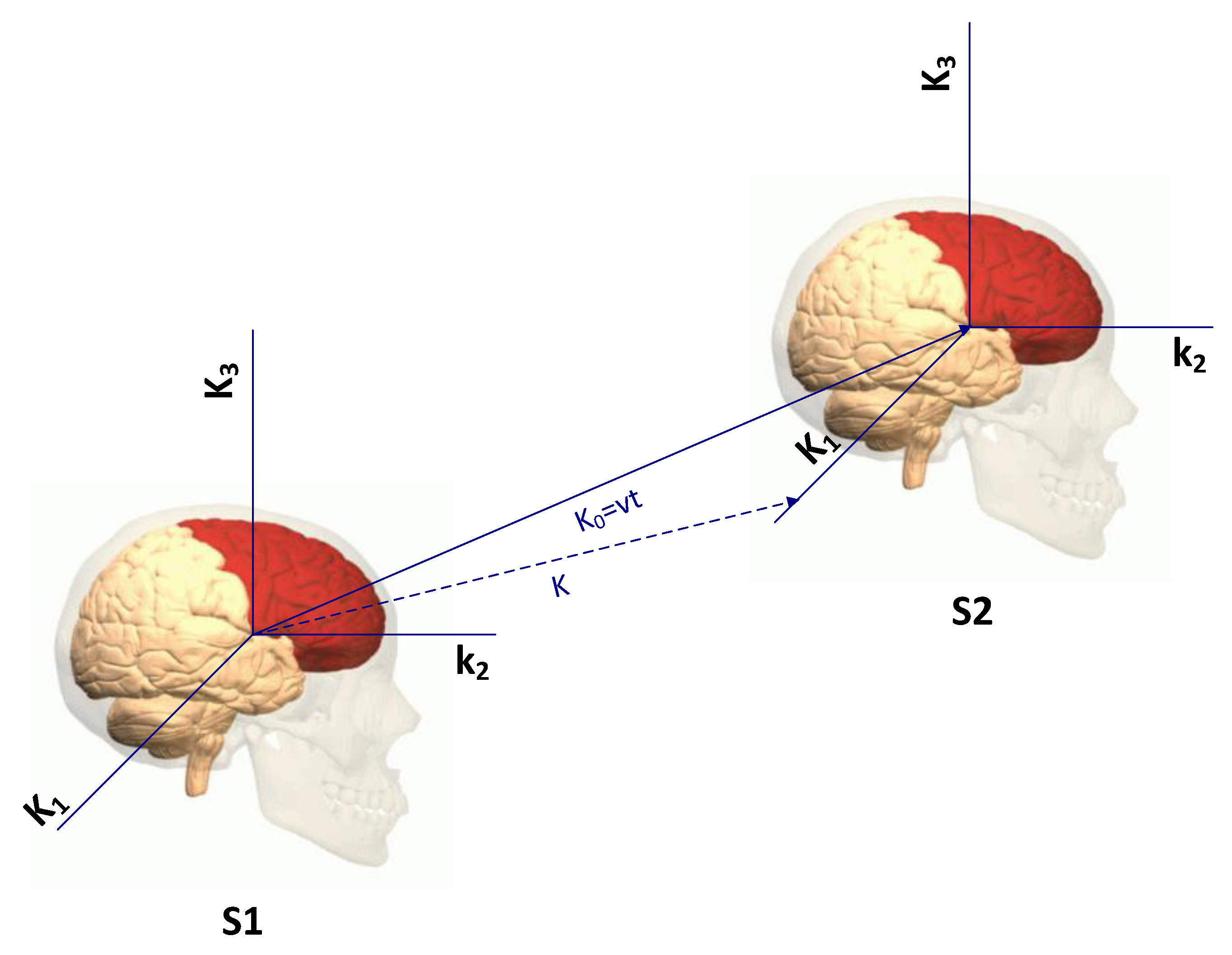
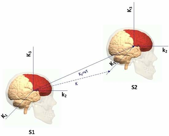
Subsequently, we study this notion. Even if the agent is in a steady state, a learning agent will form different expectations in comparison to a non-learning agent. We define this environment by a 4-dimensional vector function $\mathbf{K}={(t,K_i)}^T\in {\mathbb{R}}^4$. The function $\mathbf{K}:{\mathbb{R}}^4\to \mathbb{R}$ is continuous and twice differentiable.5 Hence, the overall knowledge space is explicitly dependent on time. This means that agents move in a spatial dimension in order to obtain a new exposure to the world. Thus, the learning agent has a 4-dimensional vector $\mathbf{K}$ that captures the essence of both dimensions: moving or learning. It is modelled by

$${\mathbf{K}}^{\prime }=T\ast \mathbf{K},$$

(3)

where ${\mathbf{K}}^{\prime }$ denotes the new knowledge space and T is a transition matrix. Matrix T is constructed by two considerations: (a) the learning agent is the same in all states of the world, i.e., $t^{\prime }=t$, and (b) the knowledge space of agent i moves from a spatial reference point $S1$ to $S2$ according to the law of physics (cf. Figure 1). Thus, we compute $K_i=K_i^{\prime }+{\dot{K}}_i\ast t$, or, after rearranging, $K_i^{\prime }=K_i-{\dot{K}}_i\ast t$. In matrix-form, we obtain

$${\mathbf{K}}^{\prime }=\left(\begin{array}{cc}1& 0\\ -{\dot{K}}_i\left(t\right)& I\end{array}\right)\ast \mathbf{K}=\left(\begin{array}{cc}1\ast t& 0\\ -{\dot{K}}_i\left(t\right)\ast t& I\ast K_i\end{array}\right),$$

where I denotes the identity matrix. Please note that the transition matrix is invertible and enables us to compute the pervious state $\mathbf{K}=T^{-1}\ast {\mathbf{K}}^{\prime }$. The transition matrix T and the inverse transition matrix $T^{-1}$ is defined by

$$T=\left(\begin{array}{cc}1& 0\\ -\dot{K_i}\left(t\right)& I\end{array}\right)⟺T^{-1}=\left(\begin{array}{cc}I& 0\\ \dot{K_i}\left(t\right)& 1\end{array}\right).$$

Proposition 1.

The expectations, $R\left(t\right)$, are time-invariant even if agent i obtains a new reference point ${\mathbf{K}}^{\prime }$.

Proof. 

Given $R\left(t\right)=N\ast \ddot{\mathbf{K}}$ and similarly $R^{\prime }\left(t\right)=N\ast \ddot{{\mathbf{K}}^{\prime }}$. Please note that $\mathbf{K}={(t,K_i\left(t\right))}^T$ is defined as a 4-dimensional vector function. Hence, the first- and second-derivative of $\mathbf{K}$ in respect to t, are

$$\frac{d\mathbf{K}}{dt}=\left(\begin{array}{c}1\\ \frac{d{K}_i}{dt}\end{array}\right)\ddot{\mathbf{K}}=\frac{d^2\mathbf{K}}{d{t}^2}=\left(\begin{array}{c}0\\ \frac{d^2{K}_i}{d{t}^2}\end{array}\right).$$

Next, we use $R\left(t\right)=N\ast \ddot{\mathbf{K}}$ and the transition matrix T. We obtain

$$\begin{array}{c}\hfill \begin{array}{cc}\hfill R\left(t\right)& =N\ast \ddot{\mathbf{K}}\hfill \\ \hfill ⟺T\ast R\left(t\right)& =N\ast T\ast \ddot{\mathbf{K}}=N\ast \left(\begin{array}{cc}1& 0\\ -{\dot{K}}_i\left(t\right)& I\end{array}\right)\ast \ddot{\mathbf{K}}\hfill \\ \hfill ⟺R^{\prime }\left(t\right)& =N\ast \ddot{{\mathbf{K}}^{\prime }}.\hfill \end{array}\end{array}$$

Consequently, we obtain the same expectations, $R^{\prime }\left(t\right)$, under the reference point ${\mathbf{K}}^{\prime }$, which proves the time-invariance. □

This proposition states that expectations are universal in all states. Suppose agent i and j are moving from state $S1$ to $S2$ vice versa from $S2$ to $S1$. In the end, both agents form the same expectations given that the knowledge space is either $\mathbf{K}$ or ${\mathbf{K}}^{\prime }$. In other words, expectations are isotropic, i.e., there is no directional dependence. Given that both agents were exposed to the same environments, they should form the same expectations.

While new in economic theory, isotropic expectations are in line with findings in cognitive sciences. Fodor (1983) claims that human expectations are based on cognitive modules that are ‘isotropic’. In cognitive sciences this property is called the theory of mind module. Similarly, Zawidszki (2013) argues that everyday reasoning is isotropic and Alechina and Logan (2010) provide empirical evidence for this finding. This novel property follows the empirical evidence of fast and frugal heuristics (Gigerenzer and Todd 1999). Heuristics are effective benchmarks in complex decision-making tasks and follow an isotropic property.6

Given the second-order differential Equation (4), we compute the 3-dimensional vector of the knowledge space, $K_i\left(t\right)$, as a solution of

$$R\left(t\right)=N\ast {\ddot{K}}_i\left(t\right),$$

(4)

given some initial state $K_i\left(0\right)=K_0$. Due to Proposition 1, we obtain the condition $\rho (K_1,K_2)=\rho (D{K}_1,D{K}_2)$, where $i=1,2$ and $D\in \mathbb{R}$ is a constant parameter. The function $\rho :{\mathbb{R}}^2\to \mathbb{R}$ is continuous in the real space.7 One can interpret the function $\rho$ as new private information that will change the knowledge space in proportion to all states, such as under a globally changing world.

Proposition 2.

The knowledge space $K_i\left(t\right)$ is isotropic, such as $\rho (K_1,K_2)=\rho (D{K}_1,D{K}_2)$.

Proof. 

This can be demonstrated by

$$\begin{array}{cc}\hfill \rho (D{K}_1,D{K}_2)& =\sqrt{{(D{K}_2-D{K}_1)}^T(D{K}_2-D{K}_1)}\hfill \\ & =\sqrt{{(K_2-K_1)}^T{D}^{T}D(K_2-K_1)}\hfill \\ & =\sqrt{{(K_2-K_1)}^T(K_2-K_1)},with{D}^{T}D=I\hfill \\ & =\rho (K_1,K_2)\hfill \end{array}$$

 □

To guarantee this property, we assume $D^{T}D=I$. Hence, the matrix D is a $3\times 3$ invertible matrix. This is a typical rotation matrix, defined by

$$D=\left(\begin{array}{ccc}1& 0& 0\\ 0& cos\left(\rho \right)& sin\left(\rho \right)\\ 0& -sin\left(\rho \right)& cos\left(\rho \right)\end{array}\right).$$

In summary, a learning agent behaves according to the following vector-differential equation

$${\mathbf{K}}^{\prime }=\left(\begin{array}{cc}1& 0\\ -v& D\end{array}\right)\mathbf{K}+{\mathbf{K}}_{\mathbf{0}},$$

(5)

where v is the speed of learning or moving and $\mathbf{K}={(t,K_i\left(t\right))}^T$ as before.

Next, we assume a fast change of the knowledge space. This is particularly the case during unexpected or sudden events (eg. a financial shock or flash crash). In such times, the knowledge space is determined by extremely fast, automatic, and unconscious processes according to cognitive sciences (Schneider and Shiffrin 1977c). Given that the neural processes have to update the knowledge space instantaneously, these updates are mostly affective. Those brain processes follow quantum physical laws and they are as fast as the speed of light.

According to the model, this implies $K_1^{\prime }=c\ast t$, where c is the speed of light. This reasoning contradicts, however, the previous finding of a learning agent and in addition special relativity theory: $K_1=K_1^{\prime }+vt=ct+vt=(c+v)\ast t$. To study this problem, we define a $4\times 4$ matrix L:

$$\begin{array}{cc}\hfill \mathbf{K}& =\left(\begin{array}{cc}\mathbb{I}& i^T\\ b& A\end{array}\right){\mathbf{K}}^{\prime }\hfill \\ & =L^{-1}{\mathbf{K}}^{\prime },\hfill \end{array}$$

(6)

where $\mathbb{I}$ is the identity matrix, $i^T$ is an identity vector8, b is a vector and A is a matrix. Both b and A remain to be determined, where $\mathbf{K}\in {\mathbb{R}}^4$. A non-learning agent stays in state $S1$ over real time $t_R$. The learning agent that is affected by the shock moves to $S2$ in time $t_M$. Of course, both time clocks are identical, but in the case of an unexpected shock the time clock of both agents are different due to the law of relativity:

$$\begin{array}{cc}\hfill {\left(c{t}_R\right)}^2& ={\left({\dot{K}}_i{t}_R\right)}^2+L^2\hfill \\ & ={\dot{K}}_i^2{t}_R^2+{\left(c{t}_M\right)}^2\hfill \\ \hfill c^2{t}_R^2& ={\dot{K}}_i^2{t}_R^2+c^2{\left(t_M\right)}^2\hfill \\ \hfill \Rightarrow t_R& =\frac{1}{\sqrt{1-\frac{{\dot{K}}_i^2}{c^2}}}{t}_M=\xi t_M,\hfill \end{array}$$

where $\xi :={(1-\frac{{\dot{K}}_i^2\left(t\right)}{c^2})}^{-1/2}$. The last expression is a time adjustment factor of the knowledge space and is similar to relativity theory.

Next, we study the impact of a learning agent by assuming a dynamic knowledge space, i.e., ${\dot{K}}_i\left(t\right)\ne 0$ with $K_i^{\prime }\left(t\right)=0$. From matrix Equation (6), we obtain $K_i\left(t_R\right)=b\ast t_M+A{K}_i^{\prime }\left(t\right)=b\ast t_M$. However, a static agent maintains the following relationship: $K_i\left(t_R\right)={\dot{K}}_i\left(t_R\right)\ast t_R$. Equating both expressions yields the unknown variable b:

$$\begin{array}{cc}\hfill K_i\left(t_R\right)=b\ast t_M+A{K}_i^{\prime }\left(t\right)=b\ast t_M& \stackrel{!}{\overbrace{=}}{\dot{K}}_i\left(t_R\right)\ast t_R\hfill \\ \hfill b& ={\dot{K}}_i\left(t_R\right)\ast \frac{t_R}{t_M}\hfill \\ \hfill b& ={\dot{K}}_i\left(t_R\right)\ast \xi .\hfill \end{array}$$

Substituting the expression for b in Equation (6), we obtain

$$\begin{array}{c}\hfill {\mathbf{K}}^{\prime }=\left(\begin{array}{cc}\xi \ast \mathbb{I}& i^T\\ -\xi {\dot{K}}_i\left(t\right)& A\end{array}\right)\mathbf{K}=L\mathbf{K},\end{array}$$

(7)

where L is a $4\times 4$ matrix.

Theorem 1.

The matrix L is invertible and has the property $L^{-1}L=\mathbb{I}$, if and only if $i^T=\frac{\xi }{c^2}{\dot{K}}_i^T\left(t\right)$ and $A=\mathbb{I}+(\xi -1)\frac{{\dot{K}}_i\left(t\right){\dot{K}}_i^T\left(t\right)}{{\dot{K}}_i^2\left(t\right)}$.

Proof. 

The details are in Appendix A. □

Finally, let us use this model in order to study the evolution of expectations. Without loss of generality, we suppose that the knowledge space is updated by private news in one dimension. This means that the expectations are affected by the first dimension, according to the vector ${\dot{K}}_i\left(t\right)={\left(\begin{array}{ccc}{\dot{k}}_{i,1}& 0& 0\end{array}\right)}^T$.

Applying Theorem 1 and substituting this in matrix L yields

$$\begin{array}{c}\hfill \begin{array}{cc}\hfill L& =\left(\begin{array}{cc}\xi & \frac{\xi }{c^2}{\left(\begin{array}{ccc}{\dot{k}}_{i,1}& 0& 0\end{array}\right)}^T\\ -\xi \ast \left(\begin{array}{c}{\dot{k}}_{i,1}\\ 0\\ 0\end{array}\right)& \left(\begin{array}{ccc}1& 0& 0\\ 0& 1& 0\\ 0& 0& 1\end{array}\right)+\frac{\xi -1}{{\dot{k}}_{i,1}^2{}_1}\left(\begin{array}{ccc}{\dot{k}}_{i,1}^2& 0& 0\\ 0& 0& 0\\ 0& 0& 0\end{array}\right)\end{array}\right)\hfill \\ & =\left(\begin{array}{cccc}\xi & -\frac{\xi }{c^2}{\dot{k}}_{i,1}& 0& 0\\ -\xi {\dot{k}}_{i,1}& \xi & 0& 0\\ 0& 0& 1& 0\\ 0& 0& 0& 1\end{array}\right).\hfill \end{array}\end{array}$$

Consequently, the new expectation and knowledge space of a moving (learning) agent i is trivially obtained by ${\mathbf{K}}^{\prime }=L\mathbf{K}$:

$$\begin{array}{c}\hfill \begin{array}{cc}\hfill t^{\prime }& =\xi t-\frac{\xi }{c^2}{\dot{k}}_{i,1}\ast k_{i,1}\hfill \\ \hfill k_{i,1}^{\prime }& =-\xi {\dot{k}}_{i,1}t+\xi k_{i,1}\hfill \\ \hfill k_{i,2}^{\prime }& =k_{i,2}\hfill \\ \hfill k_{i,3}^{\prime }& =k_{i,3}\hfill \end{array}\end{array}$$

where only $k_{i,1}^{\prime }$ changes. Interestingly, the matrix L, and thus the expectation model, behaves differently under unexpected or expected events. Consider an unexpected event, i.e., an accelerated change of agent’s i knowledge space from state $S1$ to $S2$. In this case, the time adjustment factor $\xi$ is almost 1 according to the relationship: ${\displaystyle \xi =\frac{1}{\sqrt{1-\frac{{\dot{K}}_i^2}{c^2}}}\underset{limc\gg {\dot{K}}_i}{⟶}1}$. Thus the matrix, L, transforms into

$${\displaystyle \underset{c\gg {\dot{K}}_i}{lim}}L=\widehat{L}=\left(\begin{array}{cc}1& 0\\ -{\dot{K}}_i& I\end{array}\right),$$

for $\xi /c^2=[1/\left(\xi {\dot{K}}_i\right)][{\xi }^2-1]=0$. This illustrates that the adoption of expectations under an unexpected event does not necessarily match to an expected event. Similarly, the expectation of a learning agent does not necessarily equal to the expectation of a non-learning agent. Indeed, if a learning and non-learning agent interact expectations likely differ.

4. Discussion

The quintessential part of this theory is the study of expectations in learning and non-learning agents over time t. Now we apply the model and derive newly testable hypotheses. These hypotheses are excellent topics for future experimental and empirical research.

Theorem 2.

Sudden events affect the expectation of learning agents to a great extent, and this is measured by a “yardstick of expectations” $l_{ij}\left(t\right)$.

To prove this theorem, we need preliminary propositions. First, we study the simultaneity of expectations. Consider two agents i and j, who suddenly receive news in state $S1$ ($t_1=t_2$).

Proposition 3.

Two agents i and j form the same expectations if and only if they are exposed to the same information.

Proof. 

Applying Theorem 1 permits the computation of the state $S2$. The time adjustment is

$$\begin{array}{cc}\hfill t_i^{S2}& =\xi t_i^{S1}-\frac{\xi }{c^2}{\dot{K}}_i^T{k}_i\hfill \\ \hfill t_j^{S2}& =\xi t_j^{S1}-\frac{\xi }{c^2}{\dot{K}}_j^T{k}_j.\hfill \end{array}$$

Next, subtract the first equation from the second. The time difference between both agents i and j is

$$\begin{array}{cc}\hfill t_j^{S2}-t_i^{S2}& =\xi \underset{=0}{\underbrace{(t_j^{S1}-t_i^{S1})}}-\frac{\xi }{c^2}{\dot{K}}^T(k_j-k_i)\hfill \\ \hfill \Rightarrow t_j^{S2}-t_i^{S2}& =-\frac{\xi }{c^2}{\dot{K}}^T(k_j-k_i).\hfill \end{array}$$

The last line is equivalent to zero if and only if ${\dot{K}}_i^T$ is perpendicular to $(k_j-k_i)$. This condition requires that the expectations of the agents remain constant in respect to the knowledge difference, $k_j-k_i$. If the knowledge difference remains constant, then both agents are exposed to the same information over time. This uncovers the simultaneity of expectations. □

Although this proposition demonstrates the simultaneity of expectations, the knowledge space is dynamic in reality. Thus, we consider two agents i and j with the same private and public information at time $t=0$. Yet over time, both agents develop different expectations.

Proposition 4.

Two agents i and j have the same private and public information at $t=0$. As time goes by, the expectations differ (${\dot{K}}_i^T\ne {\dot{K}}_j^T$) even if both agents have the same information environment.

Proof. 

The proof is a trivial implication of the previous proposition. In a dynamic setup there is no simultaneity of expectations. Thus, ${\dot{K}}_i^T$ is not perpendicular and, subsequently, expectations are different. □

Subsequently, we define the yardstick of expectations.

Definition 1.

The yardstick of expectations of two agents is $l_{ji}=(k_j-k_i)$. To make $l_{ji}$ positive, we define the square as $l_{ji}^2={(k_j-k_i)}^T(k_j-k_i)$.

The next proposition demonstrates a surprising property of $l_{ji}^2$ over time. This has tremendous implications for the formation of expectations and, particularly, to financial market participants.

Proposition 5.

Consider a moving agent from state $S1$ at $t_0$ to $S2$ at $t_1$. The yardstick of expectations of a moving agent declines: $l_{ji}{\left(t_1\right)}^2\le l_{ji}{\left(t_0\right)}^2$. Thus, the agent forms different expectations in contrast to a non-moving or non-learning agent. Indeed, the moving agent lives in an information-rich environment.

Proof. 

At time $t_0$, we have $l_{ji}\left(t_0\right)=k_{j,t_0}-k_{i,t_0}$. At time $t_1$, we define $l_{ji}\left(t_1\right)=A(k_{j,t_1}-k_{i,t_1})$. In square terms, it is $l_{ji}{\left(t_0\right)}^2=l_{ji}{\left(t_0\right)}^T{l}_{ji}\left(t_0\right)=l_{ji}{\left(t_1\right)}^T{A}^2{l}_{ji}\left(t_1\right)$. According to Theorem [1] matrix A is defined. The matrix $A^2$ follows trivially from Equation (A4) in Appendix A. Thus $l_{ji}{\left(t_0\right)}^2$ yields

$$\begin{array}{cc}\hfill l_{ji}{\left(t_0\right)}^2& =l_{ji}{\left(t_1\right)}^T\left[I+({\xi }^2-1)\frac{{\dot{K}}_i{\dot{K}}_i^T}{{\dot{K}}_i^2}\right]l_{ji}\left(t_1\right)\hfill \\ & =l_{ji}{\left(t_1\right)}^{T}I{l}_{ji}\left(t_1\right)+({\xi }^2-1)\frac{l_{ji}{\left(t_1\right)}^T({\dot{K}}_i{\dot{K}}_i^T)l_{ji}\left(t_1\right)}{{\dot{K}}_i^2}\hfill \\ & =l_{ji}{\left(t_1\right)}^T{l}_{ji}\left(t_1\right)+({\xi }^2-1)\frac{{({\dot{K}}_i^T{l}_{ji}\left(t_1\right))}^2}{{\dot{K}}_i^2}\hfill \\ & =l_{ji}{\left(t_1\right)}^2+({\xi }^2-1)\frac{{({\dot{K}}_i^T{l}_{ji}\left(t_1\right))}^2}{{\dot{K}}_i^2}\hfill \\ & =l_{ji}{\left(t_1\right)}^2+({\xi }^2-1)l_{ji}{\left(t_1\right)}^2.\hfill \end{array}$$

From the last line, we obtain $l_{ji}{\left(t_1\right)}^2=\frac{1}{{\xi }^2}{l}_{ji}{\left(t_0\right)}^2$. The moving agent has expectations given by ${\dot{K}}_i\to \infty$. The last term implies $\xi \to \infty$, therefore we obtain $l_{ji}{\left(t_1\right)}^2\le l_{ji}{\left(t_0\right)}^2$ □

Consequently, if both agents have the same knowledge at $t_0$ and only one agent is moving, then both will have different expectations at $t_1$. The difference of the knowledge space at $t_1$ is measured by the yardstick of expectations. Interestingly, this proposition illustrates an even stronger or remarkable point: a moving or learning agent form significantly faster expectations as the yardstick is smaller. On that account, a moving and learning agent lives in an information-rich environment because the spatial dimension exposes an agent to a new perspective even without learning. On the contrary, the non-moving but learning agent lives in an information-poor environment.

Proof of Theorem 2.

We apply Proposition (5) to prove the Theorem. The non-learning agent accumulates less information in comparison to a learning agent. This shows that agents’ expectations are prone to learning. The difference of knowledge spaces is measured by a “yardstick of expectation”. It is smaller for a moving agent and it is reliant to sudden news. Consider $t_0=\xi t_1$ and the time-change by $\Delta t_0=\xi \Delta t_1$, where $\xi =\frac{1}{\sqrt{1-\frac{{\dot{K}}_i^2}{c^2}}}\ge 1$. The time adjustment factor of a moving agent is less. Consequently, the agent needs less time to form expectations. □

We conclude:

• A moving and/or learning agent form quicker expectations, particularly in times of unexpected events;
• Expectations of non-learning agents are biased towards public information.

Of course, all hypotheses remain to be verified by experimental data in the future. Finally, there is the striking question: Does a learning agent always form better expectations? To approach this question, we conduct a brief thought experiment.

In a static environment, individual expectations are related to the mean expectation. Hence, a non-moving agent may form better expectations. Next, consider a learning agent. The learning agent forms better expectations in our theory if and only if there is an unexpected event. Indeed, Shiller (2005) finds that institutional investors, defined as high-skilled agents, do not show the pattern of changing expectations during ups and downs in comparison to ordinary investors. He attributes this time-invariant behaviour to greater professionalism.

For the first time in economic literature, we build a unified model that is corroborating robust empirical facts in behavioral and standard economics at the same time. Yet, some might still argue that the rational expectation theory is sufficient. Nonetheless, this unorthodox approach uncovers new testable hypotheses. It might be first applied in AI, particularly in the programming of reward functions with human-like face. I suggest, we let future research and data speak. Financial market data provide an excellent starting point.

5. Conclusions

Overall, this paper builds a new theory that provides innovative insights about the formation of dynamic expectations. We uncover new and testable hypotheses for future research. We do not claim that we have build a predictive model. Nevertheless, the model provides a new vantage point in comparison to standard economic theory. Furthermore, this model is suitable for the implementation in an AI approach. We find that dynamic expectations have properties, which previously have not been considered, such as the property of time-invariance, isotropy and a varying yardstick of expectations. Of course, the approach is unorthodox, however, it is intriguing. In general, more theoretical and experimental work remains to be done. This model is a first step and might open pandora’s box in order to enhance the expectation theory in economics.