Next-Day Bitcoin Price Forecast


Abstract
:1. Introduction
2. Literature Review
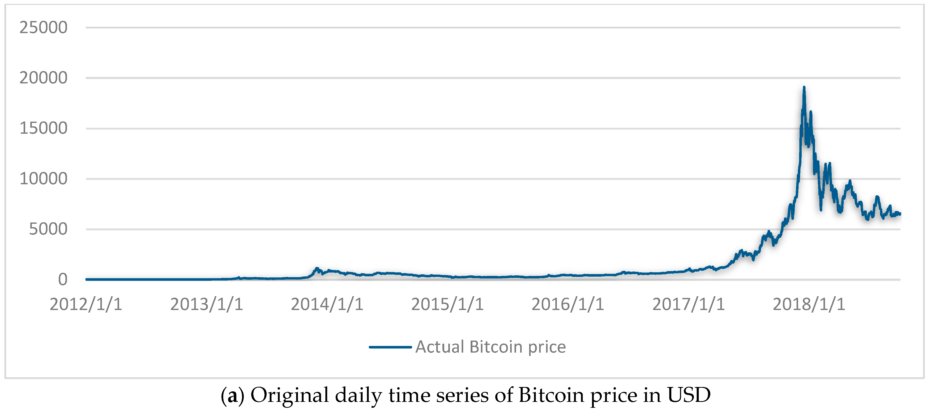
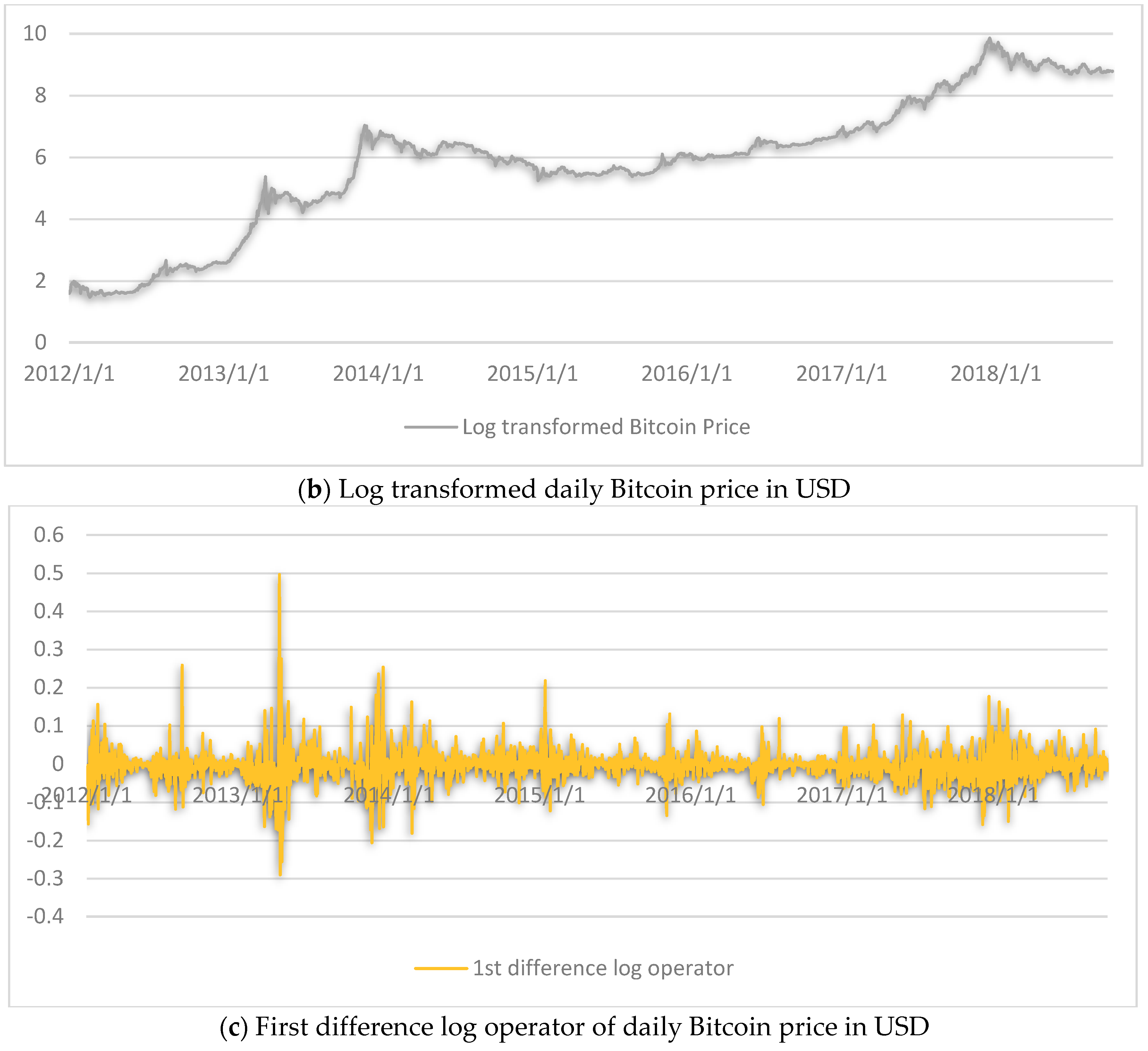
3. Data
4. Methodology
4.1. Forecast Methods
4.1.1. ARIMA
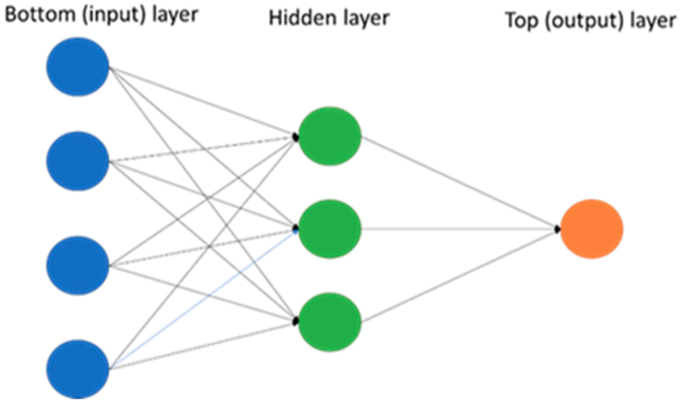
4.1.2. Neural Network Autoregression (NNAR)
4.2. Forecast Accuracy Measures
5. Empirical Results
6. Discussion and Conclusions
Author Contributions
Funding
Acknowledgments
Conflicts of Interest
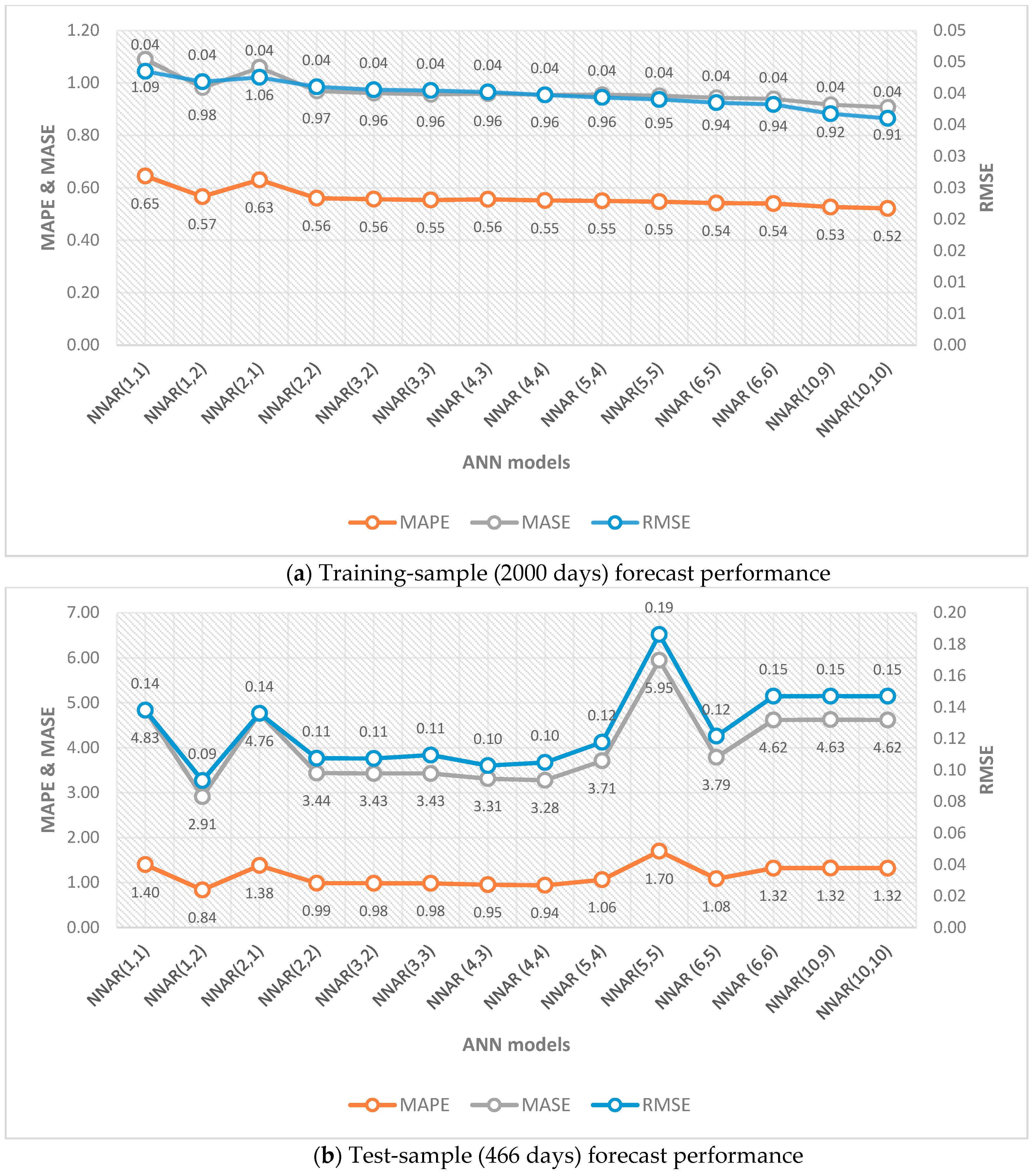
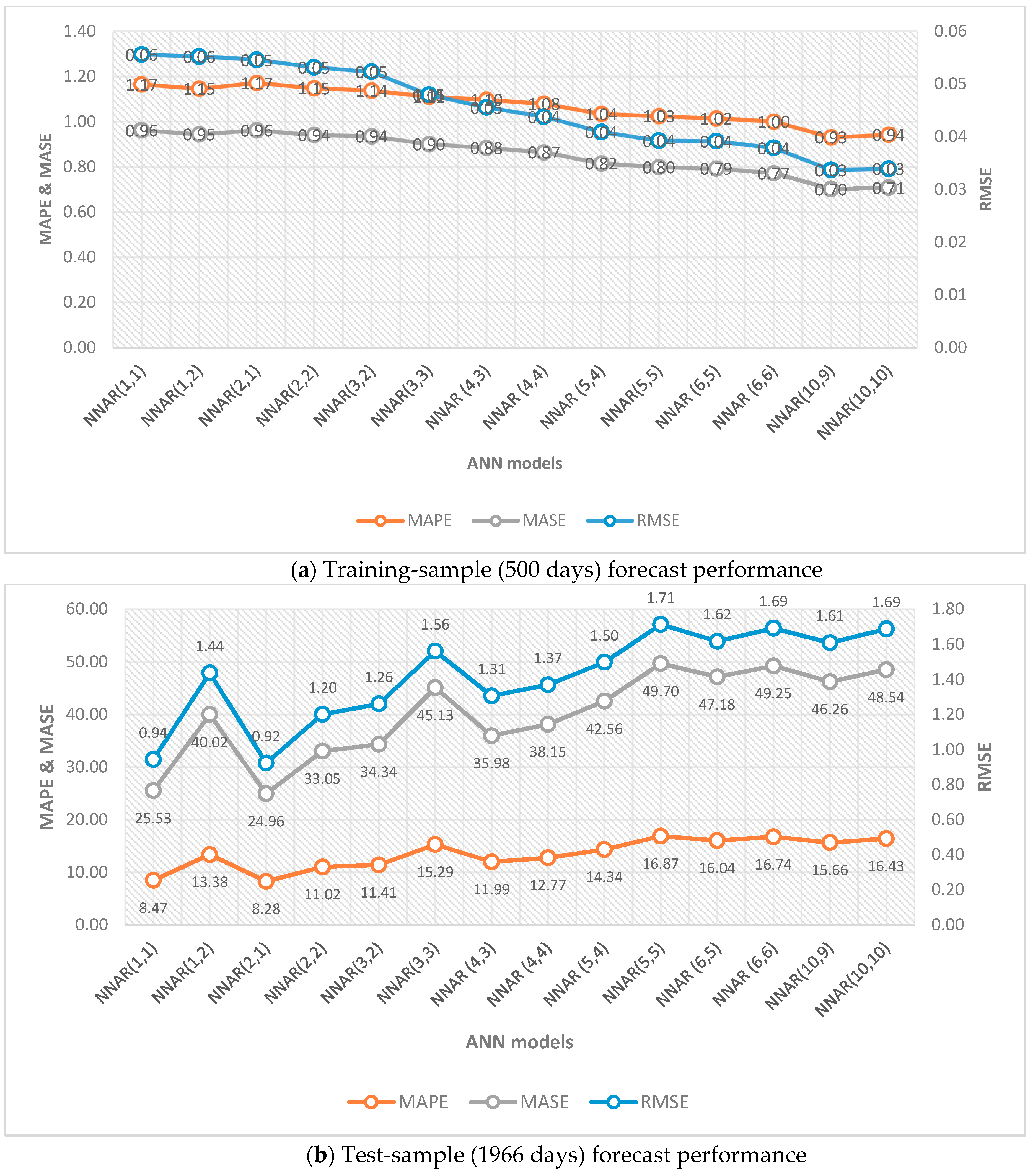
Appendix A. The 14 Estimated NNAR(p,k) Models

References
- Aalborg, Halvor Aarhus, Peter Molnár, and Jon Erik de Vries. 2018. What can explain the price, volatility and trading volume of Bitcoin? Finance Research Letters. [Google Scholar] [CrossRef]
- Abrahart, Robert J., and Linda See. 2000. Comparing neural network and autoregressive moving average techniques for the provision of continuous river flow forecasts in two contrasting catchments. Hydrological Processes 14: 2157–72. [Google Scholar] [CrossRef]
- Adya, Monica, and Fred Collopy. 1998. How effective are neural networks at forecasting and prediction? A review and evaluation. Journal of Forecasting 17: 481–95. [Google Scholar] [CrossRef]
- Alon, Ilan, Min Qi, and Robert J. Sadowski. 2001. Forecasting aggregate retail sales: A comparison of artificial neural networks and traditional methods. Journal of Retailing and Consumer Services 8: 147–56. [Google Scholar] [CrossRef]
- Álvarez-Díaz, Marcos, Manuel González-Gómez, and María Otero-Giráldez. 2018. Forecasting international tourism demand using a non-linear autoregressive neural network and genetic programming. Forecasting 1: 90–106. [Google Scholar] [CrossRef]
- Ariyo, Adebiyi Ayodele Adewumi, Ayo Oluyinka Adewumi, and Korede Charles. 2014. Stock price prediction using the ARIMA model. Paper presented at the 2014 UKSim-AMSS 16th International Conference on Computer Modelling and Simulation, Cambridge, UK, March 26–28. [Google Scholar]
- Becker, Jörg, Dominic Breuker, Tobias Heide, Justus Holler, Hans Rauer, and Rainer Böhme. 2011. The Bitcoin System. Münster. Available online: https://papers.ssrn.com/sol3/papers.cfm?abstract_id=2041492 (accessed on 5 June 2019).
- Beneki, Christina, Alexandros Koulis, Nikolaos A Kyriazis, and Stephanos Papadamou. 2019. Investigating volatility transmission and hedging properties between Bitcoin and Ethereum. Research in International Business and Finance 48: 219–27. [Google Scholar] [CrossRef]
- Benmouiza, Khalil, and Ali Cheknane. 2013. Forecasting hourly global solar radiation using hybrid k-means and nonlinear autoregressive neural network models. Energy Conversion and Management 75: 561–69. [Google Scholar] [CrossRef]
- Bouoiyour, Jamal, and Refk Selmi. 2014. What Bitcoin Looks Like? Technical Report. Munich: University Library of Munich. [Google Scholar]
- Bouoiyour, Jamal, Refk Selmi, and Aviral Tiwari. 2014. Is Bitcoin Business Income or Speculative Bubble? Unconditional vs. Conditional Frequency Domain Analysis. Munich: University Library of Munich. [Google Scholar]
- Bouri, Elie, Peter Molnár, Georges Azzi, David Roubaud, and Lars Ivar Hagfors. 2017. On the hedge and safe haven properties of Bitcoin: Is it really more than a diversifier? Finance Research Letters 20: 192–98. [Google Scholar] [CrossRef]
- Box, George Edward Pelham, and Gwilym Meirion Jenkins. 1976. Time Series Analysis: Forecasting and Control. revised ed. San Francisco: Holden-Day. [Google Scholar]
- Brandvold, Morten, Peter Molnár, Kristian Vagstad, and Ole Christian Andreas Valstad. 2015. Price discovery on Bitcoin exchanges. Journal of International Financial Markets, Institutions and Money 36: 18–35. [Google Scholar] [CrossRef]
- Brière, Marie, Kim Oosterlinck, and Ariane Szafarz. 2015. Virtual currency, tangible return: Portfolio diversification with bitcoin. Journal of Asset Management 16: 365–73. [Google Scholar] [CrossRef]
- Caporale, Guglielmo Maria, Luis Gil-Alana, and Alex Plastun. 2018. Persistence in the Cryptocurrency Market. Research in International Business and Finance 46: 141–48. [Google Scholar] [CrossRef]
- Cheah, Eng-Tuck, and John Fry. 2015. Speculative bubbles in Bitcoin markets? An empirical investigation into the fundamental value of Bitcoin. Economics Letters 130: 32–36. [Google Scholar] [CrossRef] [Green Version]
- Chen, An-Sing, Hung-Chou Chang, and Lee-Young Cheng. 2019. Time-varying Variance Scaling: Application of the Fractionally Integrated ARMA Model. The North American Journal of Economics and Finance 47: 1–12. [Google Scholar] [CrossRef]
- Chu, Jeffrey, Saralees Nadarajah, and Stephen Chan. 2015. Statistical analysis of the exchange rate of bitcoin. PLoS ONE 10: e0133678. [Google Scholar] [CrossRef] [PubMed]
- Ciaian, Pavel, Miroslava Rajcaniova, and d’Artis Kancs. 2016. The economics of BitCoin price formation. Applied Economics 48: 1799–815. [Google Scholar] [CrossRef]
- Contreras, Javier, Rosario Espinola, Francisco J. Nogales, and Antonio J. Conejo. 2003. ARIMA models to predict next-day electricity prices. IEEE Transactions on Power Systems 18: 1014–20. [Google Scholar] [CrossRef]
- Corbet, Shaen, Brian Lucey, Andrew Urquhart, and Larisa Yarovaya. 2019. Cryptocurrencies as a financial asset: A systematic analysis. International Review of Financial Analysis 62: 182–99. [Google Scholar] [CrossRef]
- Dickey, David A., and Wayne A. Fuller. 1979. Distribution of the estimators for autoregressive time series with a unit root. Journal of the American Statistical Association 74: 427–31. [Google Scholar]
- Diebold, Francis X., and Robert S Mariano. 1995. Comparing predictive accuracy. Journal of Business & Economic Statistics 13: 253–63. [Google Scholar]
- Dwyer, Gerald P. 2015. The economics of Bitcoin and similar private digital currencies. Journal of Financial Stability 17: 81–91. [Google Scholar] [CrossRef] [Green Version]
- Gujarati, Damodar N., and Dawn C. Porter. 2003. Basic Econometrics, 4th ed.New York: McGraw-Hill. [Google Scholar]
- Ho, Sui-Lau, Min Xie, and Thong Ngee Goh. 2002. A comparative study of neural network and Box-Jenkins ARIMA modeling in time series prediction. Computers & Industrial Engineering 42: 371–75. [Google Scholar]
- Hyndman, Rob J., and George Athanasopoulos. 2018. Forecasting: Principles and Practice. Melbourne: OTexts, Available online: https://otexts.com/fpp2/ (accessed on 10 March 2019).
- Hyndman, Rob John, and Yeasmin Khandakar. 2007. Automatic Time Series for Forecasting: The Forecast Package for R. Melbourne: Department of Econometrics and Business Statistics, Monash University. [Google Scholar]
- Hyndman, Rob John, and Anne B. Koehler. 2006. Another look at measures of forecast accuracy. International Journal of Forecasting 22: 679–88. [Google Scholar] [CrossRef]
- Jarque, Carlos Manuel, and Anil Kumar Bera. 1980. Efficient tests for normality, homoscedasticity and serial independence of regression residuals. Economics Letters 6: 255–59. [Google Scholar] [CrossRef]
- Katsiampa, Paraskevi. 2017. Volatility estimation for Bitcoin: A comparison of GARCH models. Economics Letters 158: 3–6. [Google Scholar] [CrossRef] [Green Version]
- Kristjanpoller, Werner, and Marcel C. Minutolo. 2018. A hybrid volatility forecasting framework integrating GARCH, artificial neural network, technical analysis and principal components analysis. Expert Systems with Applications 109: 1–11. [Google Scholar] [CrossRef]
- Kyriazis, Nikolaos A. 2019. A Survey on Efficiency and Profitable Trading Opportunities in Cryptocurrency Markets. Journal of Risk and Financial Management 12: 67. [Google Scholar] [CrossRef]
- Lam, Eric, Mathieu Benhamou, and Adrian Leung. 2018. Did Bitcoin Just Burst? How It Compares to History’s Big Bubbles. Available online: https://www.bloomberg.com/news/articles/2018-01-17/did-bitcoin-just-burst-how-it-compares-to-history-s-big-bubbles (accessed on 17 January 2018).
- Ljung, Greta Marianne, and George George Edward Pelham Box. 1978. On a measure of lack of fit in time series models. Biometrika 65: 297–303. [Google Scholar] [CrossRef]
- Miller, Jason. 2018. ARIMA Time Series Models for Full Truckload Transportation Prices. Forecasting 1: 121–34. [Google Scholar] [CrossRef]
- Molnár, Peter, Kristian Vagstad, and Ole Christian Andreas Valstad. 2015. A Bit Risky? A Comparison between Bitcoin and Other Assets using an Intraday Value at Risk Approach Working Paper. Available online: http://www.diva-portal.org/smash/get/diva2:742882/fulltext01.pdf (accessed on 5 June 2019).
- Munim, Ziaul Haque, and Hans-Joachim Schramm. 2017. Forecasting container shipping freight rates for the Far East–Northern Europe trade lane. Maritime Economics & Logistics 19: 106–25. [Google Scholar]
- Munim, Ziaul Haque, and Hans-Joachim Schramm. 2018. Forecasting container freight rates: A comparison of artificial neural network and conventional methods. Paper presented at the Annual conference of the International Association of Maritime Economists (IAME), Mombasa, Kenya, September 11–14. [Google Scholar]
- Phillips, Peter Charles Bonest, and Pierre Perron. 1988. Testing for a unit root in time series regression. Biometrika 75: 335–46. [Google Scholar] [CrossRef]
- Popper, Nathaniel. 2015. Digital Gold: Bitcoin and the Inside Story of the Misfits and Millionaires Trying to Reinvent Money. New York: Harper. [Google Scholar]
- Roberts, Jeff John. 2017. 5 Big Bitcoin Crashes: What We Learned. Fortune. Available online: https://finance.yahoo.com/news/5-big-bitcoin-crashes-learned-174604444.html (accessed on 5 June 2019).
- Robertson, Adi. 2018. Facebook Bans All Ads for Bitcoin, ICOs, and Other Cryptocurrency. Available online: https://www.theverge.com/2018/1/30/16951670/facebook-cryptocurrency-bitcoin-ico-deceptive-marketing-ban (accessed on 31 January 2018).
- Rogojanu, Angela, and Liana Badea. 2014. The issue of competing currencies: Case study–Bitcoin. Theoretical and Applied Economics 11: 103–14. [Google Scholar]
- Salisu, Afees A., Kazeem Isah, and Lateef O. Akanni. 2019. Improving the predictability of stock returns with Bitcoin prices. The North American Journal of Economics and Finance 48: 857–67. [Google Scholar] [CrossRef]
- Segendorf, Björn. 2014. What is Bitcoin? Sveriges Riksbank Economic Review 7: 71–87. Available online: http://www.riksbank.se/Documents/Rapporter/POV/2014/2014_2/rap_pov_artikel_4_1400918_eng.pdf (accessed on 5 June 2019).
- Selgin, George. 2015. Synthetic commodity money. Journal of Financial Stability 17: 92–99. [Google Scholar] [CrossRef]
- Shubik, Martin. 2014. Simecs, Ithaca Hours, Berkshares, Bitcoins and Walmarts. Cowles Foundation Discussion Paper No. 1947. Available online: https://papers.ssrn.com/sol3/papers.cfm?abstract_id=2435902 (accessed on 5 June 2019).[Green Version]
- Urquhart, Andrew. 2016. The inefficiency of Bitcoin. Economics Letters 148: 80–82. [Google Scholar] [CrossRef]
- Yermack, David. 2013. Is Bitcoin a Real Currency? An Economic Appraisal. Technical Report. National Bureau of Economic Research Working Paper No. 19747. Cambridge: National Bureau of Economic Research, Available online: https://www.nber.org/papers/w19747 (accessed on 5 June 2019).
| 1 | |
| 2 | Bitcoin price data for three days, that is, 6–8 January 2015 was not available. |


| Data | Training Sample | ADF Test | PP Test |
|---|---|---|---|
| First in-sample window (500 days) | |||
| Original data | 01/01/2012~14/05/2013 | −1.725 (0.695) | −10.597 (0.519) |
| Log transformed data | 01/01/2012~14/05/2013 | −1.478 (0.800) | −3.333 (0.919) |
| 1st difference log operator | 01/01/2012~14/05/2013 | −9.593 (0.01) | −338.72 (0.01) |
| Second in-sample window (2000 days) | |||
| Original data | 01/01/2012~25/06/2017 | 1.021 (0.99) | 6.109 (0.99) |
| Log transformed data | 01/01/2012~25/06/2017 | −1.327 (0.86) | −3.321 (0.92) |
| 1st difference log operator | 01/01/2012~25/06/2017 | −11.19 (0.01) | −1513.50 (0.01) |
| Forecast Model | Training Sample | RMSE | MAPE | MASE |
|---|---|---|---|---|
| First training-sample window (500 days) | ||||
| ARIMA (4,1,0) | 01/01/2012~14/05/2013 | 0.053 | 1.225 | 0.987 |
| NNAR (2,1) | 01/01/2012~14/05/2013 | 0.055 | 1.172 | 0.963 |
| Second training-sample window (2000 days) | ||||
| ARIMA (4,1,1) | 01/01/2012~25/06/2017 | 0.040 | 0.565 | 0.970 |
| NNAR (1,2) | 01/01/2012~25/06/2017 | 0.042 | 0.567 | 0.983 |
| Forecast Model | Test Sample | RMSE | MAPE | MASE |
|---|---|---|---|---|
| First test-sample window (1966 days) | ||||
| Forecast without re-estimation at each step | ||||
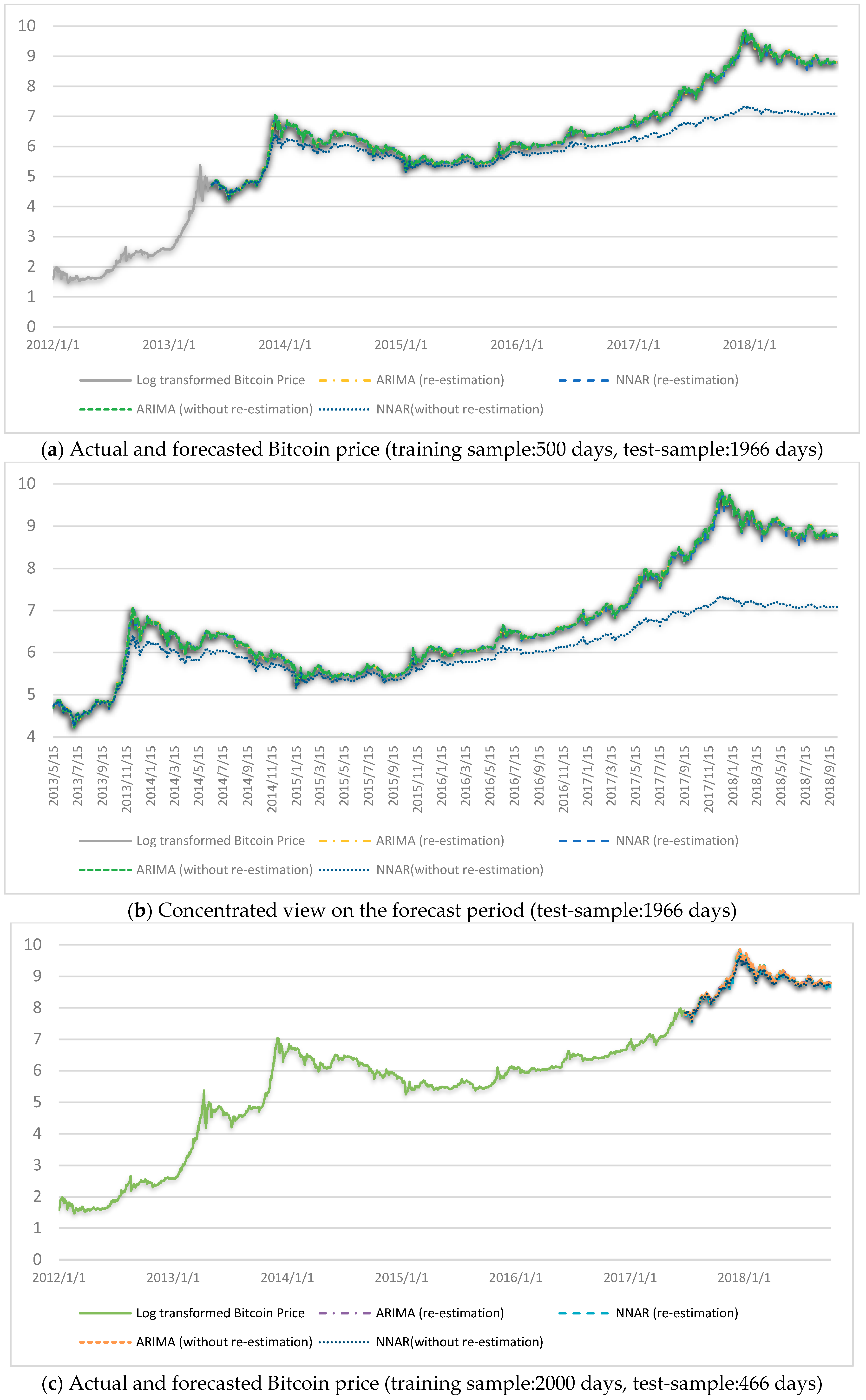
| ARIMA (4,1,0) | 15/05/2013~04/10/2018 | 0.038 | 0.379 | 0.969 |
| NNAR (2,1) | 15/05/2013~04/10/2018 | 0.924 | 8.289 | 24.990 |
| Forecast with re-estimation at each step | ||||
| ARIMA | 15/05/2013~04/10/2018 | 0.037 | 0.365 | 0.935 |
| NNAR | 15/05/2013~04/10/2018 | 0.048 | 0.453 | 1.186 |
| Second test-sample window (466 days) | ||||
| Forecast without re-estimation at each step | ||||
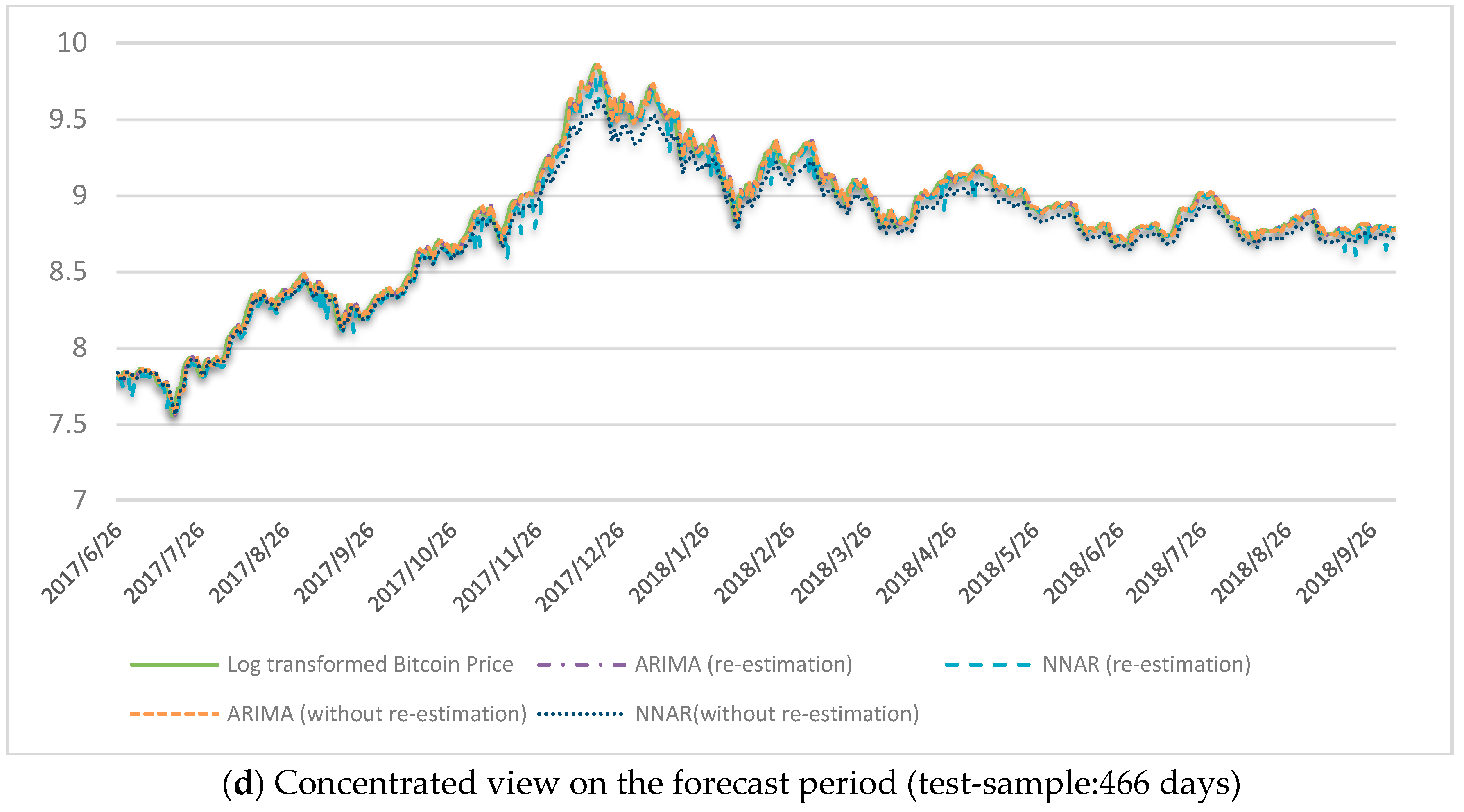
| ARIMA (4,1,1) | 26/06/2017~04/10/2018 | 0.042 | 0.354 | 1.207 |
| NNAR (1,2) | 26/06/2017~04/10/2018 | 0.093 | 0.837 | 2.911 |
| Forecast with re-estimation at each step | ||||
| ARIMA | 26/06/2017~04/10/2018 | 0.042 | 0.354 | 1.209 |
| NNAR | 26/06/2017~04/10/2018 | 0.069 | 0.537 | 1.828 |
| Models Compared | DM Statistics | p-Value |
|---|---|---|
| First test-sample window (1966 days) | ||
| ARIMA vs. NNAR (re-estimation) | −7.054 | 1.20 × 10⁻¹² |
| ARIMA vs. NNAR (without re-estimation) | −27.061 | 2.20 × 10⁻¹⁶ |
| ARIMA (re-estimation) vs. ARIMA (without re-estimation) | −4.502 | 3.56 × 10⁻⁶ |
| NNAR (re-estimation) vs. NNAR (without re-estimation) | −27.052 | 2.20 × 10⁻¹⁶ |
| Second test-sample window (466 days) | ||
| ARIMA vs. NNAR (re-estimation) | −6.006 | 1.92 × 10⁻⁹ |
| ARIMA vs. NNAR (without re-estimation) | −12.348 | 2.20 × 10⁻¹⁶ |
| ARIMA (re-estimation) vs. ARIMA (without re-estimation) | −0.785 | 0.217 |
| NNAR (re-estimation) vs. NNAR (without re-estimation) | −6.172 | 7.34 × 10⁻¹⁰ |
© 2019 by the authors. Licensee MDPI, Basel, Switzerland. This article is an open access article distributed under the terms and conditions of the Creative Commons Attribution (CC BY) license (http://creativecommons.org/licenses/by/4.0/).
Share and Cite
Munim, Z.H.; Shakil, M.H.; Alon, I. Next-Day Bitcoin Price Forecast. J. Risk Financial Manag. 2019, 12, 103. https://doi.org/10.3390/jrfm12020103
Munim ZH, Shakil MH, Alon I. Next-Day Bitcoin Price Forecast. Journal of Risk and Financial Management. 2019; 12(2):103. https://doi.org/10.3390/jrfm12020103
Chicago/Turabian StyleMunim, Ziaul Haque, Mohammad Hassan Shakil, and Ilan Alon. 2019. "Next-Day Bitcoin Price Forecast" Journal of Risk and Financial Management 12, no. 2: 103. https://doi.org/10.3390/jrfm12020103
APA StyleMunim, Z. H., Shakil, M. H., & Alon, I. (2019). Next-Day Bitcoin Price Forecast. Journal of Risk and Financial Management, 12(2), 103. https://doi.org/10.3390/jrfm12020103