Bitcoin at High Frequency


Abstract
:1. Introduction
2. Data
Data Cleaning
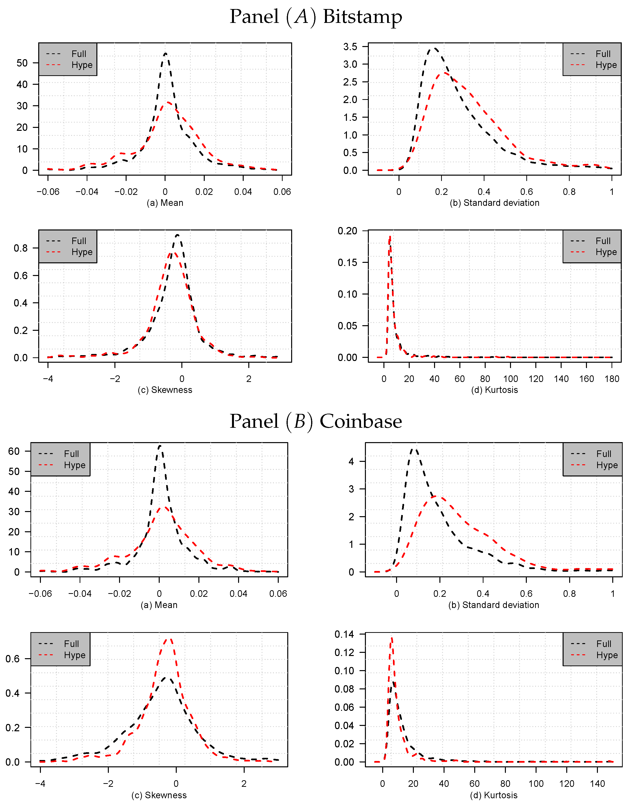
3. High Frequency Bitcoin Returns and Realized Volatiltiy
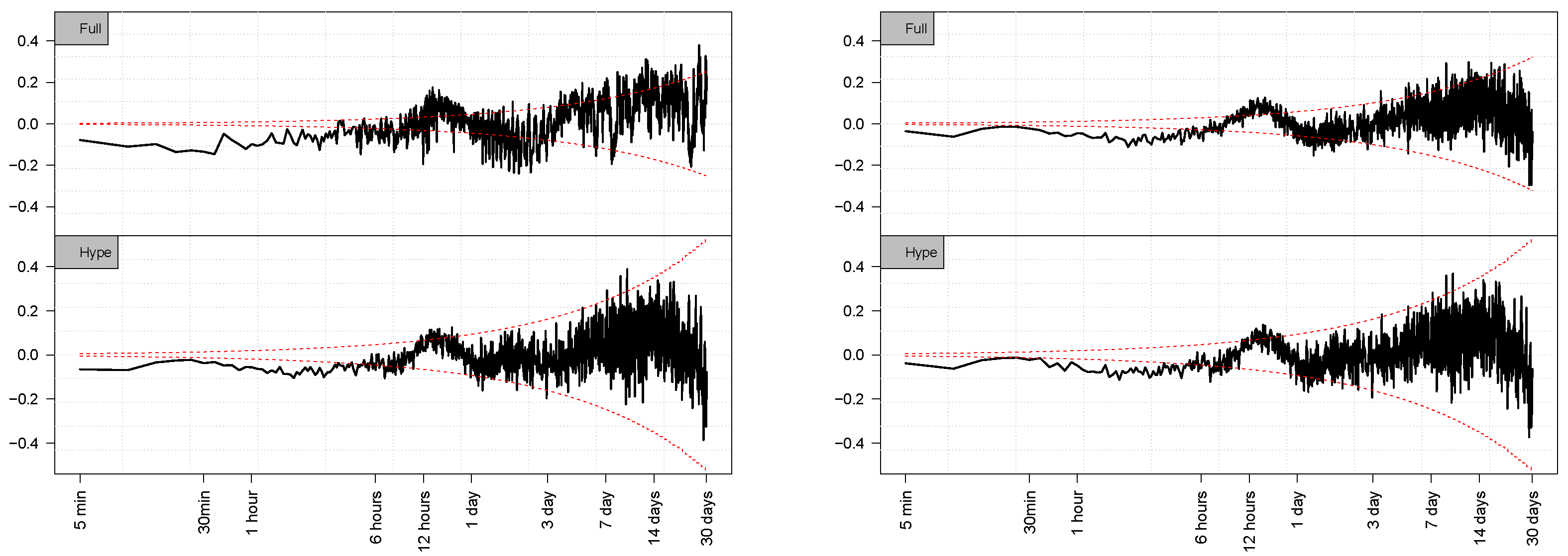
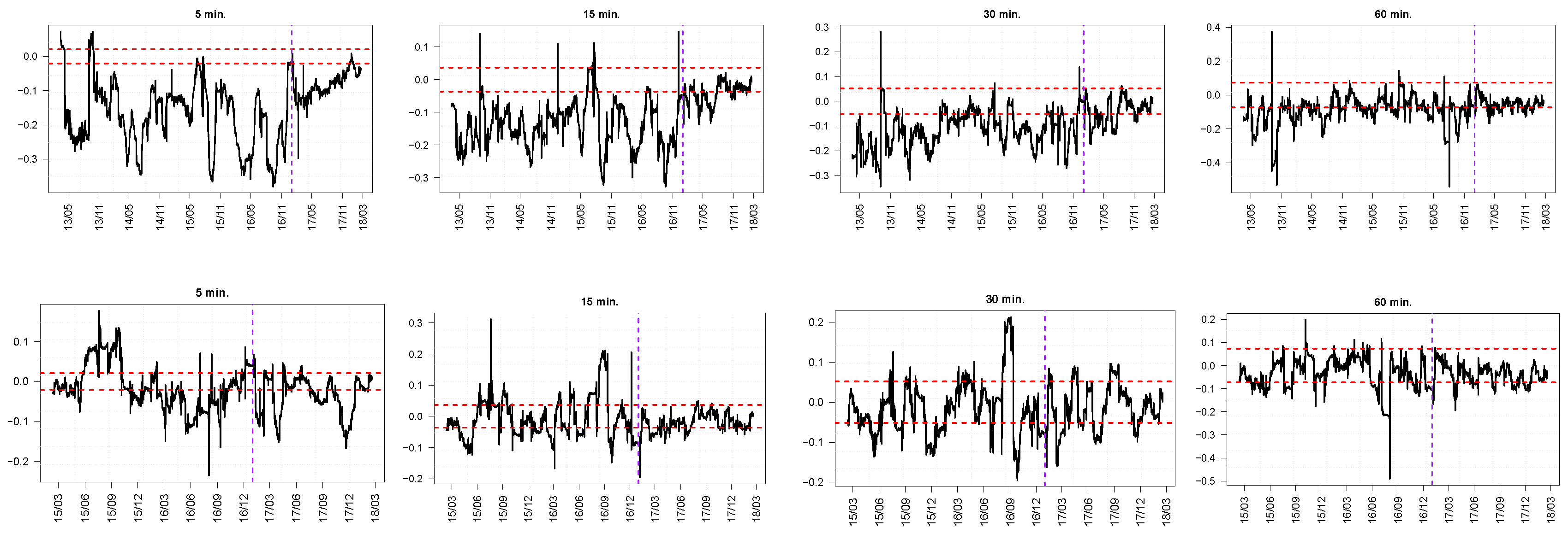
3.1. Are Bitcoin Returns Predictable?
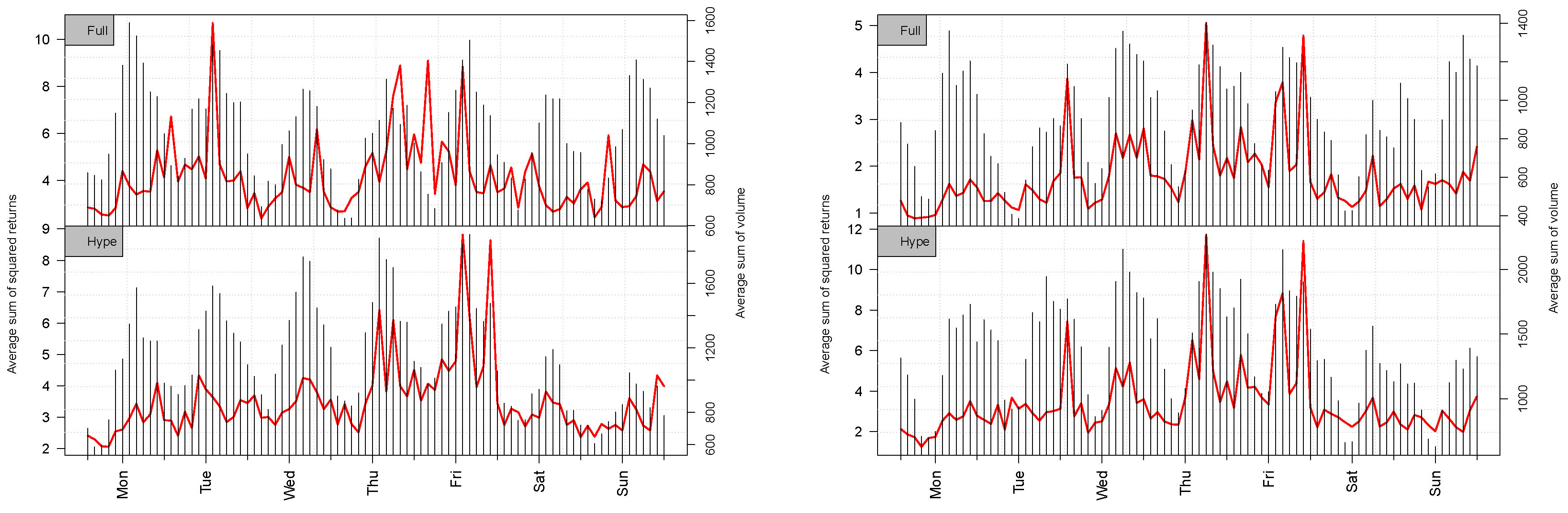
3.2. Seasonality in Bitcoin’s Volatility
4. Modelling and Predicting Bitcoin Realized Volatility
4.1. Including a Leverage Component
4.2. In Sample Results
Model Estimation
4.3. Out of Sample Results
5. Conclusions
Author Contributions
Funding
Conflicts of Interest
References
- Andersen, Torben G., Tim Bollerslev, Francis X. Diebold, and Heiko Ebens. 2001a. The distribution of realized stock return volatility. Journal of Financial Economics 61: 43–76. [Google Scholar] [CrossRef]
- Andersen, Torben G., Tim Bollerslev, Francis X. Diebold, and Paul Labys. 2001b. The distribution of realized exchange rate volatility. SSRN Electronic Journal 27: 42–55. [Google Scholar]
- Andersen, Torben G., Tim Bollerslev, and Francis X. Diebold. 2007. Roughing it up: Including jump components in the measurement, modeling, and forecasting of return volatility. Review of Economics and Statistics 89: 701–20. [Google Scholar] [CrossRef]
- Ardia, David, Keven Bluteau, Kris Boudt, and Leopoldo Catania. 2018. Forecasting risk with markov-switching garch models: A large-scale performance study. International Journal of Forecasting 34: 733–47. [Google Scholar] [CrossRef]
- Ardia, David, Keven Bluteau, and Maxime Rüede. 2018. Regime changes in Bitcoin GARCH volatility dynamics. Finance Research Letters. [Google Scholar] [CrossRef]
- Balcilar, Mehmet, Elie Bouri, Rangan Gupta, and David Roubaud. 2017. Can volume predict bitcoin returns and volatility? A quantiles-based approach. Economic Modelling 64: 74–81. [Google Scholar] [CrossRef]
- Bariviera, Aurelio F. 2017. The inefficiency of bitcoin revisited: A dynamic approach. Economics Letters 161: 1–4. [Google Scholar] [CrossRef]
- Barndorff-Nielsen, Ole, Peter R. Hansen, Asger Lunde, and Neil Shephard. 2009. Realized kernels in practice: trades and quotes. Econometrics Journal 12: C1–C32. [Google Scholar] [CrossRef]
- Barndorff-Nielsen, Ole E. 2004. Power and bipower variation with stochastic volatility and jumps. Journal of Financial Econometrics 2: 1–37. [Google Scholar] [CrossRef]
- Barndorff-Nielsen, Ole E., and Neil Shephard. 2003. Realized power variation and stochastic volatility models. Bernoulli 9: 243–65. [Google Scholar] [CrossRef]
- Barndorff-Nielsen, Ole E., Svend Erik Graversen, Jean Jacod, Mark Podolskij, and Neil Shephard. 2006. A central limit theorem for realised power and bipower variations of continuous semimartingales. In From Stochastic Calculus to Mathematical Finance. Berlin/Heidelberg: Springer, pp. 33–68. [Google Scholar]
- Bauwens, Luc, Christian M. Hafner, and Sébastien Laurent. 2012. Handbook of Volatility Models and Their Applications. New York: John Wiley & Sons, vol. 3. [Google Scholar]
- Black, Fischer. 1976. Studies of Stock Price Volatility Changes. In Proceedings of the 1976 Meeting of the Business and Economic Statistics Section. Washington: American Statistical Association, pp. 177–181. [Google Scholar]
- Bloomberg. 2017. Nasdaq Plans to Introduce Bitcoin Futures. Available online: https://www.bloomberg.com/news/articles/2017-11-29/nasdaq-is-said-to-plan-bitcoin-futures-joining-biggest-rivals (accessed on 10 February 2019).
- Breedon, Francis, and Angelo Ranaldo. 2013. Intraday patterns in FX returns and order flow. Journal of Money, Credit and Banking 45: 953–65. [Google Scholar] [CrossRef]
- Brownlees, Christian T., and Giampiero M. Gallo. 2006. Financial econometric analysis at ultra-high frequency: Data handling concerns. Computational Statistics & Data Analysis 51: 2232–245. [Google Scholar]
- Catania, Leopoldo, and Stefano Grassi. 2017. Modelling crypto-currencies financial time-series. SSRN Electronic Journal. [Google Scholar] [CrossRef]
- Catania, Leopoldo, Stefano Grassi, and Francesco Ravazzolo. 2019. Forecasting cryptocurrencies under model and parameter instability. International Journal of Forecasting 35: 485–501. [Google Scholar] [CrossRef]
- Catania, Leopoldo, Stefano Grassi, and Francesco Ravazzolo. 2018. Predicting the volatility of cryptocurrency time–series. In Mathematical and Statistical Methods for Actuarial Sciences and Finance: MAF 2018. Edited by Marco Corazza, María Durbán, Aurea Grané, Cira Perna and Marilena Sibillo. New York: Springer. [Google Scholar]
- CME. 2017. CME Group Announces Launch of Bitcoin Futures. Available online: http://www.cmegroup.com/media-room/press-releases/2017/10/31/cme_group_announceslaunchofbitcoinfutures.html (accessed on 10 February 2019).
- Corsi, Fulvio. 2008. A simple approximate long-memory model of realized volatility. Journal of Financial Econometrics 7: 174–96. [Google Scholar] [CrossRef]
- Corsi, Fulvio, Francesco Audrino, and Roberto Renò. 2012. HAR modeling for realized volatility forecasting. In Handbook of Volatility Models and Their Applications. Hoboken: John Wiley & Sons, Inc., pp. 363–82. [Google Scholar]
- Creal, Drew, Siem Jan Koopman, and André Lucas. 2013. Generalized Autoregressive Score Models with Applications. Journal of Applied Econometrics 28: 777–95. [Google Scholar] [CrossRef]
- Cryptocoinsnews. 2017. Tokyo Financial Exchange Plans for Bitcoin Futures Launch. Available online: https://www.cryptocoinsnews.com/breaking-tokyo-financial-exchange-plans-bitcoin-futures-launch/ (accessed on 10 February 2019).
- Dacorogna, Michael M., Ulrich A. Müller, Robert J. Nagler, Richard B. Olsen, and Olivier V. Pictet. 1993. A geographical model for the daily and weekly seasonal volatility in the foreign exchange market. Journal of International Money and Finance 12: 413–38. [Google Scholar] [CrossRef]
- Diebold, Francis, and Robert Mariano. 1994. Comparing Predictive Accuracy. Journal of Business and Economic Statistics 13: 253–65. [Google Scholar]
- Dyhrberg, Anne H. 2016. Bitcoin, gold and the dollar—A GARCH volatility analysis. Finance Research Letters 16: 85–92. [Google Scholar] [CrossRef]
- Gencay, Ramazan, Michel Dacorogna, Ulrich A. Muller, Richard Olsen, and Olivier Pictet. 2001. An Introduction to High-Frequency Finance. Amsterdam: Elsevier Science Publishing Co. Inc. [Google Scholar]
- Hansen, Peter R., and Asger Lunde. 2005. A forecast comparison of volatility models: Does anything beat a garch (1, 1)? Journal of Applied Econometrics 20: 873–89. [Google Scholar] [CrossRef]
- Harvey, Andrew C. 2013. Dynamic Models for Volatility and Heavy Tails: With Applications to Financial and Economic Time Series. Cambridge: Cambridge University Press, Vol. 52. [Google Scholar]
- Katsiampa, Paraskevi. 2017. Volatility estimation for bitcoin: A comparison of GARCH models. Economics Letters 158: 3–6. [Google Scholar] [CrossRef]
- Liu, Lily, Andrew Patton, and Kevin Sheppard. 2015. Does anything beat 5-minute rv? A comparison of realized measures across multiple asset classes. Journal of Econometrics 187: 293–311. [Google Scholar] [CrossRef]
- Marcellino, Massimiliano, James H. Stock, and Mark W. Watson. 2006. A comparison of direct and iterated multistep ar methods for forecasting macroeconomic time series. Journal of econometrics 135: 499–526. [Google Scholar] [CrossRef]
- Nakamoto, Satoshi. 2009. Bitcoin: A Peer-to-Peer Electronic Cash System. Available online: https://bitcoin.org/bitcoin.pdf (accessed on 10 February 2019).
- Nelson, Daniel B. 1991. Conditional heteroskedasticity in asset returns: A new approach. Econometrica: Journal of the Econometric Society 59: 347–70. [Google Scholar] [CrossRef]
- Phillip, Andrew, Jennifer S. K. Chan, and Shelton Peiris. 2018. A new look at cryptocurrencies. Economics Letters 163: 6–9. [Google Scholar] [CrossRef]
- Stavroyiannis, Stavros. 2018. Value-at-risk and related measures for the bitcoin. The Journal of Risk Finance 19: 127–136. [Google Scholar] [CrossRef]
- Taylor, Stephen J., and Xinzhong Xu. 1997. The incremental volatility information in one million foreign exchange quotations. Journal of Empirical Finance 4: 317–40. [Google Scholar] [CrossRef]
- Zakoian, Jean-Michel. 1994. Threshold Heteroskedastic Models. Journal of Economic Dynamics and Control 18: 931–55. [Google Scholar] [CrossRef]
- Zhang, Yuanyuan, Stephen Chan, Jeffrey Chu, and Saralees Nadarajah. 2019. Stylised facts for high frequency cryptocurrency data. Physica A: Statistical Mechanics and Its Applications 513: 598–612. [Google Scholar] [CrossRef]
| 1. | Specifically, 54.42% for the Bitstamp exchange and 68.78% for the Coinbase exchange. |
| 2. | Among several exchanges where Bitcoin is traded we have selected two of the most active ones. Another possibility would have been to consider GDAX instead of Coinbase since this exchange might give a better representation of Bitcoin. However, we have decided to use Coinbase since, differently from GDAX and Bitstamp which are traditional exchanges, it is a click and buy exchange which allows investor to immediately invest in Bitcoin. We thank an anonymous referee for pointing out this to us. |
| 3. | See also Balcilar et al. (2017) who examine the causal relation between Bitcoin return/volatility and traded volumes. |
| 4. | However, we acknowledge that at the time of writing there is a lag of 10.83 min between the placement and execution of a trade on Bitstamp. Differently, on Coinbase trade execution is immediate. |
| 5. | Please note that Bitcoin is traded 7 days a week. |


| Bitstamp | |||||||||
| Number of outliers | 141,029 | 134,584 | 128,934 | 104,018 | 99,007 | 85,593 | 82,623 | 78,603 | 75,438 |
| Average outliers per day | 0.51% | 0.46% | 0.42% | 0.38% | 0.34% | 0.30% | 0.31% | 0.27% | 0.25% |
| Coinbase | |||||||||
| Number of outliers | 118,162 | 107,936 | 100,570 | 98,037 | 89,922 | 84,009 | 85,499 | 78,482 | 73,521 |
| Average outliers per day | 0.24% | 0.20% | 0.17% | 0.19% | 0.16% | 0.14% | 0.17% | 0.14% | 0.12% |
| Bitstamp | Coinbase | |||
|---|---|---|---|---|
| Full Sample | Hype | Full Sample | Hype | |
| Raw observations | 22,346,195 | 12,217,195 | 39,285,138 | 27,126,897 |
| Volume | 1112 | 98 | 0 | 0 |
| Outliers | 104,295 | 61,350 | 103,071 | 85,418 |
| Simultaneous ticks | 9,976,748 | 5,338,296 | 28,400,400 | 18,861,682 |
| Final sample size in seconds | 12,263,584 | 6,817,445 | 10,781,667 | 8,179,797 |
| Trading days | 1825 | 442 | 1132 | 442 |
| Mean | Standard Deviation | |||||||
|---|---|---|---|---|---|---|---|---|
| 2015 | 2016 | 2017 | 2018 | 2015 | 2016 | 2017 | 2018 | |
| S&P 500 | 16.67 | 15.83 | 11.09 | 16.64 | 4.34 | 3.97 | 1.36 | 5.09 |
| Coinbase | 11.25 | 6.89 | 37.24 | 59.02 | 29.76 | 17.26 | 78.46 | 67.15 |
| Bitstamp | 23.10 | 10.08 | 37.46 | 64.88 | 72.48 | 14.69 | 57.19 | 62.44 |
| Bitstamp | Coinbase | |||
|---|---|---|---|---|
| Full | Hype | Full | Hype | |
| Maximum | 61.09 | 7.41 | 10.62 | 10.62 |
| Minimum | −36.89 | −15.54 | −21.02 | −21.02 |
| Mean | 0.00 | 0.00 | 0.00 | 0.00 |
| Median | 0.00 | 0.00 | 0.00 | 0.00 |
| Std. Dev. | 0.31 | 0.33 | 0.20 | 0.31 |
| Skewness | −0.28 | −0.38 | −0.58 | −0.40 |
| Excess of kurtosis | 8.84 | 8.28 | 14.36 | 10.22 |
| Bitstamp | Coinbase | |||||||||||
|---|---|---|---|---|---|---|---|---|---|---|---|---|
| Maximum | 9374.99 | 96.82 | 9.15 | 1320.43 | 36.34 | 7.19 | 835.73 | 28.91 | 6.73 | 326.73 | 18.08 | 5.79 |
| Minimum | 0.87 | 0.93 | −0.14 | 0.12 | 0.35 | 0.12 | 0.01 | 0.31 | −2.31 | 0.02 | 0.15 | 0.02 |
| Mean | 54.94 | 5.23 | 2.86 | 7.35 | 1.85 | 1.29 | 21.47 | 3.41 | 1.82 | 2.69 | 1.25 | 0.88 |
| Median | 15.63 | 3.95 | 2.75 | 2.01 | 1.42 | 1.10 | 5.81 | 2.41 | 1.76 | 1.02 | 1.00 | 0.70 |
| Std. Dev. | 311.15 | 5.26 | 1.23 | 45.42 | 1.98 | 0.87 | 53.93 | 3.14 | 1.57 | 11.48 | 1.06 | 0.73 |
| Skewness | 21.19 | 7.39 | 0.69 | 21.16 | 7.96 | 1.82 | 7.51 | 2.72 | 0.19 | 24.81 | 5.51 | 1.34 |
| Kurtosis | 541.82 | 94.59 | 4.11 | 552.17 | 102.12 | 8.60 | 81.77 | 14.48 | 2.55 | 694.19 | 74.09 | 5.77 |
| J.test | 239 | 7612 | ||||||||||
| Bitstamp | Coinbase | |||||||||||
|---|---|---|---|---|---|---|---|---|---|---|---|---|
| Maximum | 588.38 | 24.26 | 6.38 | 37.84 | 6.15 | 3.66 | 835.73 | 28.91 | 6.73 | 326.73 | 18.08 | 5.79 |
| Minimum | 1.40 | 1.19 | 0.34 | 0.26 | 0.51 | 0.23 | 0.23 | 0.48 | −1.48 | 0.07 | 0.26 | 0.06 |
| Mean | 42.23 | 5.64 | 3.18 | 4.62 | 1.91 | 1.44 | 41.04 | 5.21 | 2.89 | 5.16 | 1.78 | 1.30 |
| Median | 24.56 | 4.96 | 3.20 | 2.90 | 1.70 | 1.36 | 18.70 | 4.32 | 2.93 | 2.19 | 1.48 | 1.16 |
| Std. Dev. | 58.99 | 3.23 | 1.06 | 5.37 | 0.99 | 0.72 | 76.98 | 3.73 | 1.29 | 21.39 | 1.42 | 0.76 |
| Skewness | 4.44 | 1.80 | 0.06 | 3.10 | 1.32 | 0.53 | 5.49 | 2.30 | −0.06 | 14.05 | 6.77 | 1.41 |
| Kurtosis | 31.60 | 8.08 | 2.86 | 16.08 | 5.49 | 2.90 | 43.11 | 10.97 | 3.16 | 210.54 | 73.42 | 7.91 |
| J. test | 714 | 31,853 | 1562 | |||||||||
| HAR-RV | HAR-RV-J | HAR-RV-L | HAR-RV-CJ | HAR-RV-CJ-L | |||||||||||
|---|---|---|---|---|---|---|---|---|---|---|---|---|---|---|---|
| c | |||||||||||||||
| adj. | |||||||||||||||
| HAR-RV | HAR-RV-J | HAR-RV-L | HAR-RV-CJ | HAR-RV-CJ-L | |||||||||||
|---|---|---|---|---|---|---|---|---|---|---|---|---|---|---|---|
| c | |||||||||||||||
| 26% | |||||||||||||||
| adj. | 26% | ||||||||||||||
| Daily | |||||||||||||||||||||||
|---|---|---|---|---|---|---|---|---|---|---|---|---|---|---|---|---|---|---|---|---|---|---|---|
| Model | RW | HAR-RV | HAR-RV-J | HAR-RV-L | HAR-RV-CJ | HAR-RV-CJ-L | |||||||||||||||||
| MAFE | |||||||||||||||||||||||
| RMSFE | |||||||||||||||||||||||
| Weekly | |||||||||||||||||||||||
| Model | RW | HAR-RV | HAR-RV-J | HAR-RV-L | HAR-RV-CJ | HAR-RV-CJ-L | |||||||||||||||||
| MAFE | |||||||||||||||||||||||
| RMSFE | 072 | ||||||||||||||||||||||
| Monthly | |||||||||||||||||||||||
| Model | RW | HAR-RV | HAR-RV-J | HAR-RV-L | HAR-RV-CJ | HAR-RV-CJ-L | |||||||||||||||||
| MAFE | |||||||||||||||||||||||
| RMSFE | |||||||||||||||||||||||
| Daily | |||||||||||||||||||||||
|---|---|---|---|---|---|---|---|---|---|---|---|---|---|---|---|---|---|---|---|---|---|---|---|
| Model | RW | HAR-RV | HAR-RV-J | HAR-RV-L | HAR-RV-CJ | HAR-RV-CJ-L | |||||||||||||||||
| MAFE | |||||||||||||||||||||||
| RMSFE | |||||||||||||||||||||||
| Weekly | |||||||||||||||||||||||
| Model | RW | HAR-RV | HAR-RV-J | HAR-RV-L | HAR-RV-CJ | HAR-RV-CJ-L | |||||||||||||||||
| MAFE | |||||||||||||||||||||||
| RMSFE | |||||||||||||||||||||||
| Monthly | |||||||||||||||||||||||
| Model | RW | HAR-RV | HAR-RV-J | HAR-RV-L | HAR-RV-CJ | HAR-RV-CJ-L | |||||||||||||||||
| MAFE | |||||||||||||||||||||||
| RMSFE | |||||||||||||||||||||||
© 2019 by the authors. Licensee MDPI, Basel, Switzerland. This article is an open access article distributed under the terms and conditions of the Creative Commons Attribution (CC BY) license (http://creativecommons.org/licenses/by/4.0/).
Share and Cite
Catania, L.; Sandholdt, M. Bitcoin at High Frequency. J. Risk Financial Manag. 2019, 12, 36. https://doi.org/10.3390/jrfm12010036
Catania L, Sandholdt M. Bitcoin at High Frequency. Journal of Risk and Financial Management. 2019; 12(1):36. https://doi.org/10.3390/jrfm12010036
Chicago/Turabian StyleCatania, Leopoldo, and Mads Sandholdt. 2019. "Bitcoin at High Frequency" Journal of Risk and Financial Management 12, no. 1: 36. https://doi.org/10.3390/jrfm12010036
APA StyleCatania, L., & Sandholdt, M. (2019). Bitcoin at High Frequency. Journal of Risk and Financial Management, 12(1), 36. https://doi.org/10.3390/jrfm12010036