Identification of Core Suppliers Based on E-Invoice Data Using Supervised Machine Learning

Abstract

Since not all suppliers are to be managed in the same way, a purchasing strategy requires proper supplier segmentation so that the most suitable strategies can be used for different segments. Most existing methods for supplier segmentation, however, either depend on subjective judgements or require significant efforts. To overcome the limitations, this paper proposes a novel approach for supplier segmentation. The objective of this paper is to develop an automated and effective way to identify core suppliers, whose profit impact on a buyer is significant. To achieve this objective, the application of a supervised machine learning technique, Random Forests (RF), to e-invoice data is proposed. To validate the effectiveness, the proposed method has been applied to real e-invoice data obtained from an automobile parts manufacturer. Results of high accuracy and the area under the curve (AUC) attest to the applicability of our approach. Our method is envisioned to be of value for automating the identification of core suppliers. The main benefits of the proposed approach include the enhanced efficiency of supplier segmentation procedures. Besides, by utilizing a machine learning method to e-invoice data, our method results in more reliable segmentation in terms of selecting and weighting variables.

1. Introduction

Successful supply chain management (SCM) requires the effective and efficient management of a purchasing strategy (Bensaou 1999; Gelderman and van Weele 2002; Park et al. 2010). The purchasing strategy has assumed an increasingly prominent role with the growing importance of SCM (Chen et al. 2004). Consequently, the impact of the purchasing function on a company’s competitive advantage has also increased (Wagner and Johnson 2004; Park et al. 2010).

Acknowledging that not all suppliers are to be managed in the same way, a purchasing strategy requires proper supplier segmentation so that the most suitable strategies can be used for different segments (Hallikas et al. 2005; Gelderman and van Weele 2002). Supplier segmentation, usually taking place after supplier selection, is defined as the process of classifying suppliers in different segments (Rezaei and Ortt 2013). Since Parasuraman (1980) introduced the first conceptual model, two distinct approaches have been developed: One is the continuum approach (e.g., Ellram 1991; Cox 1996; Lambert et al. 1996; Dyer et al. 1998), which bases supplier segmentation on a continuum of supplier relations. The other is the portfolio approach, introduced by Kraljic (1983). The portfolio approach classifies suppliers or purchase items into four portfolio quadrants and, then, suggests differentiated purchasing strategies for the quadrants. In the portfolio model, Kraljic (1983) proposed the profit impact and supply risk dimensions for classification. Compared with the continuum approach, the portfolio approach has been more popular in both academia and practice (Gelderman and van Weele 2003; Montgomery et al. 2017). The portfolio approach has also evolved toward a hybrid model that includes the continuum approach (e.g., Olsen and Ellram 1997; Bensaou 1999; Svensson 2004; Caniëls and Gelderman 2005; Hallikas et al. 2005).

Despite the influence of the portfolio approach, it has drawn some criticism. One of the main limitations lies in its qualitative nature which results in the subjective building of the portfolio (Padhi et al. 2012; Montgomery et al. 2017). The weighting and positioning suppliers in the quadrants are the most important, but subjective elements of the portfolio model (Olsen and Ellram 1997; Montgomery et al. 2017), which makes the process more vulnerable. Second, selecting the dimensions of a portfolio is challenging, and the factors that determine the dimensions are difficult to obtain (Padhi et al. 2012). Even for the Kraljic’s portfolio model, the factors that determine the dimensions are arguable. Besides, giving weights to the factors is another challenge.

To overcome these limitations, this paper proposes a novel approach for supplier segmentation. The objective of this paper is to develop an automated and effective way to identify core suppliers, whose profit impact on a buyer is significant. To achieve this objective, the application of a supervised machine learning technique, Random Forests (RF), to e-invoice data is proposed. The proposed method has been applied to real e-invoice data obtained from an automobile parts manufacturer, and its effectiveness has been validated.

Our proposed method is envisioned to be of value for automating supplier segmentation procedures. To our best knowledge, no attempt has been made to automate supplier segmentation procedures. The main benefits of the proposed method include the enhanced efficiency of supplier segmentation procedures. Thanks to the use of e-invoice data, all the necessary data can be automatically collected. In existing methods, the data collection procedure is the most time-consuming process. Another benefit is that our method is more reliable in terms of selecting and weighting variables. E-invoice data are some of the most comprehensive data that can be used in supplier segmentation as they contain all the details of transactions between a supplier and a buyer. Therefore, utilizing e-invoice data can provide more reliable segmentation results. In addition, the proposed method is more robust to human bias, as a machine learning algorithm determines the importance of input variables.

The remainder of this paper is organized as follows. In Section 2, previous research on supplier segmentation and e-invoice is reviewed. Section 3 explains our methods for identifying core suppliers. In Section 4, the results of a case study are presented. Finally, Section 5 provides implications of this paper and Section 6 concludes our work and discusses directions of future work.

2. Literature Review

2.1. Supplier Segmentation

Since Parasuraman (1980) introduced the first conceptual model, several models of supplier segmentation have been presented in the literature. These models can largely be divided into two categories (Hallikas et al. 2005). The first approach is based on the continuum of supplier relationships. Ellram’s (1991) model classified relationships as duration and governance structure. Cox (1996) suggested a continuum of supplier relationships from arm’s length to strategic alliance. Dyer et al. (1998) developed a more explicit supplier segmentation method based on the differences between outsourcing strategies. In the study, two types of supplier relationships were suggested: (1) durable arm’s length; and (2) strategic partnership.

The second approach is the portfolio model, which is widely accepted in both academia and practice. Kraljic (1983) introduced the first portfolio model, where two dimensions (profit impact and supply risk) are used to classify suppliers. Kraljic’s (1983) model, known as the Kraljic Portfolio Matrix (KPM), has been the most widely accepted portfolio model (Caniëls and Gelderman 2005; Montgomery et al. 2017). The KPM is defined as a 2 × 2 matrix, categorizing four quadrants of purchasing items or suppliers (Gelderman and Semeijn 2006; Montgomery et al. 2017). It then suggests differentiated approaches for these categories of suppliers. The KPM approach has proved to be an effective tool for visualizing and illustrating purchasing strategies. Arguably, it has been the most diagnostic and prescriptive tool available for purchasing functions (Wagner et al. 2013).

The KPM has evolved toward including the continuum approach based on supplier–buyer relationships. Caniëls and Gelderman (2005) presented an empirical study that aimed to test the power and dependence of buyer–supplier relationships, using the data from a survey of purchasing professionals. Svensson (2004) combined the continuum and portfolio approach, where a supplier’s commitment and commodity’s importance were used to classify suppliers. Bensaou (1999) classified suppliers in accordance with the levels of the buyer’s and the supplier’s specific investments. Olsen and Ellram’s (1997) approach uses the strength of the relationship and the relative supplier attractiveness. Hallikas et al. (2005) considered the supplier and buyer dependency risks in their portfolio model.

Empirical studies have also shown the usefulness of the KPM (Carter 1997; Gelderman and van Weele 2002; Wagner and Johnson 2004). Gelderman and Mac Donald (2008) applied the KPM to logistic applications. The application of the KPM has been extended to the construction and healthcare industries (Ferreira et al. 2015; Medeiros and Ferreira 2018).

Despite the influence of the portfolio approach, it has drawn some criticism. One of the main limitations lies in its qualitative nature which results in the subjective building of the matrix (Padhi et al. 2012; Montgomery et al. 2017). The weighting and positioning suppliers in the quadrants are the most important, but a subjective element of the portfolio model (Olsen and Ellram 1997; Montgomery et al. 2017), which makes the process more challenging and quesitonable. Moreover, it requires significant effort to gather expert opinions and surveys. Another limitation is that the selection of the portfolio dimensions is vulnerable (Hallikas et al. 2005). While Kraljic (1983) proposed profit impact and supply risk as their criteria, different portfolio dimensions have been suggested by several models (e.g., Bensaou (1999); Olsen and Ellram (1997); Masella and Rangone (2000); Svensson (2004); and Hallikas et al. (2005)) and the argument of the portfolio dimensions continues.

To overcome the qualitative nature of the portfolio approach, Olsen and Ellram (1997), Liu and Xu (2008), and Padhi et al. (2012) suggested a less subjective model for configuring the quadrants; however, to some extent, limitations still exist (Montgomery et al. 2017). Montgomery et al. (2017) suggested a multi-objective decision analysis (MODA) model based on the organization’s data to quantify the KPM. While these approaches provide more quantified models, they still require considerable effort to position suppliers in the matrix. In addition, the selection of variables in each dimension and the results of classification need to be validated. In summary, although several portfolio models have been developed in supplier segmentation and strategic planning, there are still some limitations to overcome.

2.2. E-Invoice

E-invoices, also called electronic invoices, are a form of electronic billing. They are issued, transmitted, and received electronically via the Internet (Lian 2015). The European Union introduced a regulation for e-invoices in 2001, and this was adopted by European countries first. Despite some obstacles, including security concerns and the potential for fraud, a growing number of countries are accepting the application of e-invoices (Keifer 2011; Lian 2015). South Korea also enacted the e-invoicing regulation in 2011.

A typical e-invoice contains:

-

Date of the invoice;

-

Name and contact details of the supplier and buyer;

-

Description and unit price of the product; and

-

The total amount charged.

The benefits of e-invoicing include: (1) enhanced transparency of transactions; (2) automated invoice validation; (3) enhanced spend management; and (4) enhanced account reconciliation (Keifer 2011). Besides, e-invoicing facilitates the collection of purchasing data. The benefits of e-invoices are yet to be fully exploited, as research on e-invoicing has been limited to service adoption (Lian 2015), system development, and implementation (Suwisuthikasem and Tangsripairoj 2008; Chang et al. 2013).

E-invoices provide one of the most crucial and comprehensive data that should be considered in a supplier–buyer relationship, as they encompass all the transaction details between a supplier and a buyer. Thus, the use of e-invoice data in establishing purchasing strategies deserves attention. In this paper, the use of e-invoices is explored to identify core suppliers using a machine learning algorithm. Prior to the application of a machine learning algorithm, the raw e-invoice data should be transformed into a proper input format, which is detailed in the next section.

3. Methods

3.1. Overview

Figure 1 shows the overall procedures to identify core suppliers based on e-invoice data through a supervised machine learning technique, namely RF. In this research, a core supplier is defined as a supplier whose impact on a buyer is significant. Therefore, the strategic and leverage suppliers in the KPM can be classified as core suppliers.

From a machine learning perspective, identifying core suppliers can be regarded as a classification problem, where a target variable is a binary variable that indicates whether a supplier is a core supplier. The first step of the procedure is data collection; e-invoice transactional data between suppliers and a target company should be collected and organized by supplier. Next, the data should be labeled to facilitate their use by supervised machine learning. As it requires expertise to label core suppliers, expert interviews or surveys are recommended to label the data. Prior to applying a machine learning algorithm, input variables—presented in the following section—are defined as objectives of the problem. Then, the raw data, obtained from e-invoice data, are preprocessed and transformed into suitable data formats. Then, the commonly used ensemble classification technique, RF, is applied to the preprocessed data.

3.2. Random Forests (RF)

Among the commonly used machine learning algorithms for a classification problem are decision trees (DTs), support vector machines (SVMs) and neural networks (NNs) (Kotsiantis 2007). While DTs are simple and intuitive, they can have an instability problem, where small changes in input training samples can cause large changes in output (Li and Belford 2002). The performance of NNs and SVMs can largely depend on the sufficiency of input data; they show decent performances as long as sufficient input data are provided (Zhang et al. 1998). In addition, further elaboration is required for the parameter tuning of NNs and SVMs. Based on classification trees, a RF algorithm is an ensemble learning method for classification. RF is known for their decent performance compared with many other classifiers such as DTs, NNs, and SVMs. Other advantages of RF include its ease of use and its robustness to overfitting (Breiman 2001; Liaw and Wiener 2002; Brown and Mues 2012). Furthermore, it is known that RFs are more appropriate for “large p, small n” problems (Ishwaran et al. 2010). Given that the number of suppliers of a single company is usually no more than the order of thousands, our classification problem can be regarded as a “small n” problem. Therefore, RF is selected as the machine learning method with which to classify the suppliers.

RF is a popular tree-based ensemble learning method for classification and regression, wherein several decision trees (weak learners) are constructed, and the decision trees’ habit of overfitting to their training sets is corrected. It produces outputs by aggregating the predictions of the randomly selected trees (Liaw and Wiener 2002). In this study, 200,000 trees are used; 70% of the available data are allocated for training and the remaining 30% are used for testing. Cross-validation is utilized to evaluate the predictive performance of the model.

3.3. Data Preprocessing

In this section, the list of input variables for a supervised machine learning algorithm is explained. Note that all of the input variables are generated for each supplier, not each item.

3.3.1. Total Cost of Purchase

Total cost of purchase is one of the main internal factors with which to evaluate the importance of suppliers (Kraljic 1983; Padhi et al. 2012; Montgomery et al. 2017). Total cost of purchase is the total purchase cost from a supplier during the analysis period.

3.3.2. Transaction Frequency/Cycle

It can be assumed that, as transactions increase in frequency, suppliers tend to commit themselves to a strong, long-term relationship with their buyers (Williamson 1979; Lai et al. 2005; Ramon-Jeronimo and Florez-Lopez 2018). Thus, the transaction frequency and cycle of a supplier can be used to evaluate their importance (Barney and Ouchi 1986; Anderson and Narus 1990). Transaction frequency is defined as the total number of transactions with a supplier during the analysis period. The transaction cycle is measured as the average and standard deviation of intervals between transactions with a supplier. Suppose a supplier made six transactions with a buyer during the analysis period, the transaction frequency of the supplier is six and the transaction cycle is measured as the average and standard deviation of the five intervals between transactions.

3.3.3. Percentage of Critical Items

According the Pareto’s law, a few critical items account for most of the purchase cost. Thus, a supplier whose transaction is focused on the critical items can be assumed to be of interest. In this study, the ratio of the purchase cost of the top three item categories to the total purchase cost is used as an input variable.

3.3.4. Duration of Partnership

A long-term partnership between a supplier and a buyer suggests trust between the two companies (Bensaou 1999). Thus, the duration of partnership can be used in our model. Duration of partnership is defined as the time duration between the first and last transactions with a supplier.

3.3.5. Monthly Purchase over the Last 12 Months

In addition to the total purchase cost of a supplier, the monthly purchase pattern can reveal more detailed information. Thus, an array of monthly purchase cost of a supplier over the last 12 months is selected as an input variable.

3.3.6. Synchronization Index

A supplier’s impact on a buyer’s business growth is one of the factors that determine the importance of a supplier (Kraljic 1983; Montgomery et al. 2017). Revenue and total purchase are the key measures that determine the business growth of a buyer. Thus, in addition to the transaction amount, the correlation of a supplier’s transactions to a buyer’s inbound or outbound transactions deserves consideration. If a supplier’s transaction patterns synchronize well with the revenue and the total purchase pattern of a buyer, the supplier’s impact on the buyer can be assumed. To calculate the synchronization, a dynamic time warping (DTW) algorithm is adopted. The DTW algorithm, which is widely used owing to its robustness against missing data points (Mueen and Keogh 2016), computes the similarity of two time series (Berndt and Clifford 1994; Tormene et al. 2009).

Calculating the synchronization index also requires consideration of time lags, as it takes time for purchase transactions to generate revenue. It has been estimated that the average inventory turns in the automobile industry is 9.9 turns per year, meaning that it takes an average of 1.2 months to turn the inventory (Mayer 2014). In this study, time lags of one and three months are used to calculate the synchronization between the time series: the monthly purchase from a supplier and the monthly revenue of a buyer.

Table 1. Input variables.

No.	Name	Description	Type
1	TCP	Total cost of purchase: Total purchased cost from a supplier during the analysis period.	Numeric
2	FREQ	Transaction Frequency: Total number of transactions with a supplier during the analysis period.	Numeric
3	CYCLE1	Transaction Cycle: Average interval between transactions with a supplier.	Numeric
4	CYCLE2	Transaction Cycle: Standard deviation of intervals between transactions with a supplier.	Numeric
5	C_ITEM	Percentage of critical items’ transaction: Supplier’s ratio of the purchase cost of the top three item categories to the total purchase cost.	Numeric
6	DUR	Duration of partnership: Time duration between the first and the last transaction with a supplier	Numeric
7	{M1,M2,…, M12}	Monthly purchases over the last 12 months: monthly purchase cost of a supplier over the last 12 months. Mj denotes a monthly purchase j months ago.	Numeric
8	PR_SYN1	Synchronization index: Similarity between a monthly purchase of a supplier’s primary item and a monthly purchase of a buyer.	Numeric
9	PR_SYN2	Synchronization index: Similarity between a monthly purchase from a supplier and a monthly purchase of a buyer.	Numeric
10	SL_SYN1 {L1, L3}	Synchronization index: Similarity between a monthly purchase of a supplier’s primary item and a monthly revenue of a buyer. L1 indicates a one-month time lag and L3 indicates a three-month time lag.	Numeric
11	SL_SYN1 {L1, L3}	Synchronization index: Similarity between a monthly purchase from a supplier and a monthly revenue of a buyer. L1 indicates a one-month time lag and L3 indicates a three-month time lag.	Numeric

summarizes the input variables used in the model.

4. Case Study Results

4.1. Case: Automobile Components Manufacturer

The proposed approach has been applied to a Korean manufacturer of automobile components. Founded in 1985, the company manufactures brake pads and lining products. As one of the major players in the Korean brake-pad industry, the company posted US$ 147 Million in revenue for 2017. In this study, e-invoice data for five years, namely from 1 January 2013 to 31 December 2017, were collected, preprocessed, and used as inputs for RF. A total of 3378 e-invoice data were collected and 125 suppliers were identified.

Prior to the application of RF, expert surveys were conducted to label the suppliers. The necessary statistics and supplier information were provided to industry experts and their evaluation of supplier importance was surveyed using a Likert five-point scale. A supplier with more than four points on the scale was labeled as a core supplier. As a result, 36 out of 125 suppliers were labeled as core suppliers.

4.2. Results

RFs were applied to the preprocessed dataset to predict the core suppliers of the company. A total of 200,000 trees were used in the model. For each tree, 70% of the data were used as a training dataset and the rest were used as out-of-bag (OOB) data, that is, a test dataset. Of the 25 input variables, five were randomly selected in each tree because it is recommended to select the square root of the number of input variables in each tree (Breiman 2002).

Classification was performed on a dataset obtained from the automobile parts manufacturer. To evaluate the results, most commonly used measures such as accuracy, recall, and precision were used along with a weighted F1 score. As shown in

Table 2. Confusion matrix.

		Actual Class
		Core Supplier	Non-Core Supplier
Predicted Class	Core Supplier	TP (True Positive)	FP (False Positive)
	Non-Core Supplier	FN (False Negative)	TN (True Negative)

Note: “True positive” means the case for correctly predicted core suppliers, while “false positive” means the case for incorrectly predicted core suppliers. “True negative” means the case for correctly predicted non-core suppliers, while “false negative” means the case for incorrectly predicted non-core suppliers.

, performance measures can be defined according to the confusion matrix of our classification problem.

Accuracy, recall, and precision measures are defined as follows (Luong and Dokuchaev 2018; Hamori et al. 2018):

$$\mathrm{Accuracy}=\frac{\mathrm{TP}+\mathrm{TN}}{\mathrm{TP}+\mathrm{FP}+\mathrm{TN}+\mathrm{FN}},$$

(1)

$$\mathrm{Precision}=\frac{\mathrm{TP}}{\mathrm{TP}+\mathrm{FP}},\mathrm{and}$$

(2)

$$\mathrm{Recall}=\frac{\mathrm{TP}}{\mathrm{TP}+\mathrm{FN}}.$$

(3)

A weighted F1 score was used to adjust the cut-off (threshold) value for classification.

$$\mathrm{Weighted}\mathrm{F}1=2\frac{\left(1+{\beta }^2\right)·precision·recall}{precision+{\beta }^2·recall} .$$

(4)

In practice, recall is more important than precision since it is better to retrieve as many core suppliers as possible, while accepting some false positive errors. Thus, our model adjusted the threshold value with respect to the weighted F1 score with beta = 1.1, meaning an increased emphasis on recall.

The experimental results of the RF classification are given in

Table 3. Case study results.

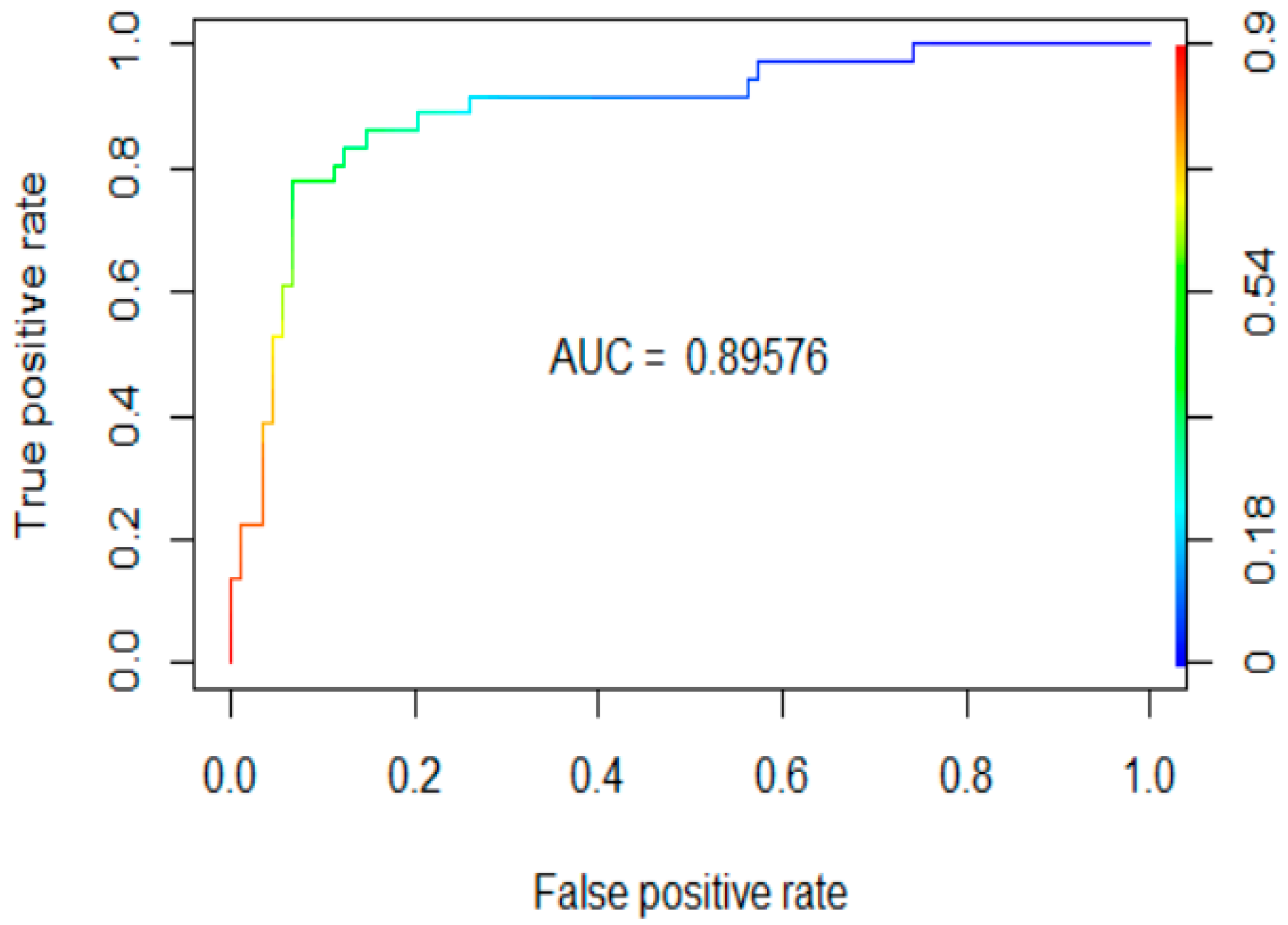
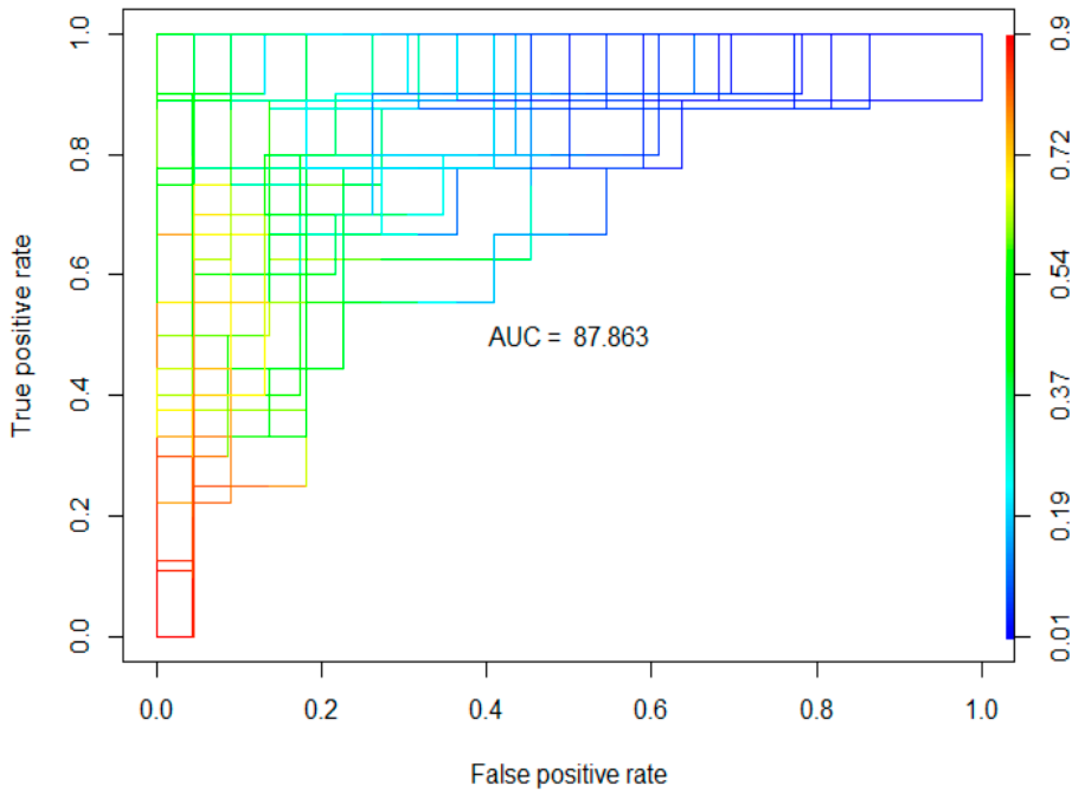
Test Data	Threshold	Accuracy	Weighted F1-Score	Recall	Precision	AUC
OOB	0.5	84.38 (3.16)	71.84 (6.23)	69.63 (7.82)	74.41(5.23)	89.58
	0.47	85.26 (3.83)	76.94 (4.96)	84.62 (6.7)	71.24 (7.96)
Cross-validation	0.5	81.71 (7.09)	66.52 (12.18)	63.56 (14.98)	72.76 (15.92)	87.86 (7.3)
	0.47	80.4 (11.13)	70.43 (11.81)	78.14 (16.77)	67.68 (16.99)

Note: Numbers in parenthesis denote standard deviations resulting from repetitions.

. Note that the threshold was adjusted to 0.47 to increase the recall and weighted F1 score. A four-fold cross-validation was used and repeated 30 times to evaluate the predictive performance of the model. As shown in the table, the adjustment of the threshold resulted in an enhanced recall score. Comparing the increased recall with the decreased precision, the adjustment seems to be worth consideration. The results indicate that the RF performs well in identifying core suppliers. The cross-validation results confirm the predictive performance of the model.

As shown in Figure 2 and Figure 3, the receiver operating characteristic (ROC) curves were created by plotting the true positive rate (TPR) against the false positive rate (FPR). The area under the curve (AUC) of OOB data is 89.58 and the average AUC of cross-validation is 87.86.

To examine the importance of input variables, two measures were used. The first measure calculates variable importance as mean decrease in accuracy using the out-of-bag observations (Archer and Kimes 2008). The second measure is the mean decrease in the Gini impurity of RF (Liaw and Wiener 2002). As can be seen in Figure 4, the total cost of purchase (TCP) is the most important variable, followed by the synchronization indices (PR_SYN1, PR_SYN2, and SL_SYN1_L3). Transaction frequency (FREQ) and cycle (CYCLE1) also indicate their importance.

5. Implications

Even though supplier segmentation is a fundamental element of purchasing strategies, the limitations of existing methods have generated obstacles in practice. The main contribution of our study is the enhanced efficiency of supplier segmentation procedures. The enhancement is mainly due to the use of e-invoice data, which enabled automated data collection. Another contribution is that our method overcomes the subjective nature of existing methods, thus providing more reliable classification results. As a machine learning algorithm determines the importance of input variables, our model can be less prone to subjective judgement errors.

Among several criteria for supplier segmentation, this paper focuses on profit impact, as it has been one of the crucial dimensions supported by a number of models (e.g., Kraljic 1983; Choi and Hartley 1996; Van Weele 2010; Gelderman and Mac Donald 2008; Padhi et al. 2012; Montgomery et al. 2017). Although we have adopted one dimension of the KPM, the advantages of the proposed model can have following ramifications.

The benefit of automating the supplier segmentation procedures can be more evident for small- and medium-sized enterprises (SMEs). Even though an SME’s need for an appropriate purchasing strategy is no less than that of a large conglomerate, time and money constraints often cause hesitation in implementing a purchasing portfolio. Therefore, our method can facilitate the adoption of a purchasing portfolio model in practice.

Another implication of our method is a dynamic perspective of supplier segmentation. Most supplier segmentation methods assume a static perspective (Rezaei and Ortt 2013), which is far from reality. However, the proposed method can overcome such limitation. As e-invoice data can be updated and re-trained by a machine learning algorithm, our method can reflect changes in the business environment. In addition, the accuracy of our method would further improve with the updates of e-invoice data.

Besides, our model can be used for the default prediction of a supply chain, as it can be easily extended to identifying the networks of core suppliers. The default problem of propagating through a supply chain can be a significant concern for both original equipment manufacturers (OEMs) and lending institutions (Hamori et al. 2018). In particular, the financial default of suppliers is one of the major concerns in the automotive industry (Wagner et al. 2009).

6. Conclusions

This paper presented a novel approach to automating the identification of core suppliers, through the use of machine learning techniques and e-invoice data. To examine the effectiveness of our approach, e-invoice data of an automobile parts manufacturer and its suppliers were utilized. The results of high accuracy and the area under the curve (AUC) results attested to the applicability of the proposed method. It is expected that the accuracy would further improve, as more e-invoice data are collected.

Despite the contributions of the present study, there are some limitations which need to be acknowledged. Item-level classification could not be considered due to the limitation of e-invoice data. It has been observed that item descriptions of e-invoice data, in particular, are often missing or inconsistent. The item-level data were compromised, making it difficult to apply them to our model; thus, they were excluded from the analysis. However, with the enhanced integrity of e-invoice data, our model can be extended to the item-level analysis.

As the focus of this paper is the utilization of e-invoice data for a purchasing strategy, the scope of this paper is constrained to identifying core suppliers, not a full KPM. The profit impact is regarded as an internal factor, whereas the supply risk is an external factor (Montgomery et al. 2017). Since e-invoice data encompass the transactional data between a supplier and a buyer, it is mainly concerned with the internal factor. In fact, constructing a KPM requires simultaneous consideration of the two factors; considering the impact factor alone cannot provide a complete KPM. However, identifying core suppliers can still be a basic and fundamental step toward a purchasing strategy. Given supplier risk and external data with the advancement of big data technologies, our model can be applied to the determination of a complete KPM, which is a suitable future research topic.

Another future research topic is the application of the proposed model to the construction of a core supplier network, from a target company to an upstream or downstream supply chain, and the prediction of the default risk of the target company or the entire supply chain.

References

- Anderson, James C., and James A. Narus. 1990. A Model of Distributor Firm and Manufacturer Firm Working Partnerships. Journal of Marketing 54: 42–58. [Google Scholar] [CrossRef]
- Archer, Kellie J., and Ryan V. Kimes. 2008. Empirical characterization of random forest variable importance measures. Computational Statistics and Data Analysis 52: 2249–60. [Google Scholar] [CrossRef]
- Barney, Jay B., and William G. Ouchi. 1986. Organizational Economics. San Francisco: Jossey-Bass. [Google Scholar]
- Bensaou, Mustapha. 1999. Portfolios of Buyer-Supplier Relationships. Sloan Management Review 40: 35. [Google Scholar]
- Berndt, Donald, and James Clifford. 1994. Using dynamic time warping to find patterns in time series. Workshop on Knowledge Discovery in Databases 398: 359–70. [Google Scholar]
- Breiman, Leo. 2001. Random Forests. Machine Learning 45: 5–32. [Google Scholar] [CrossRef]
- Breiman, Leo. 2002. Manual-Setting up, Using, and Understanding Random Forests. Available online: https://www.stat.berkeley.edu/~breiman/Using_random_forests_v4.0.pdf (accessed on 11 August 2018).
- Brown, Iain, and Christophe Mues. 2012. An experimental comparison of classification algorithms for imbalanced credit scoring data sets. Expert Systems with Applications 39: 3446–53. [Google Scholar] [CrossRef]
- Caniëls, Marjolein C. J., and Cees J. Gelderman. 2005. Purchasing strategies in the Kraljic matrix—A power and dependence perspective. Journal of Purchasing and Supply Management 11: 141–55. [Google Scholar] [CrossRef]
- Carter, Joseph R. 1997. Supply positioning at SGX Corporation. Best Practices in Purchasing and Supply Chain Management 1: 5–8. [Google Scholar]
- Chang, Chin-Jui, Huai-Chien Kuo, Chen-Yuan Chen, Tsung-Hao Chen, and Pei-Yin Chung. 2013. Retracted: Ergonomic Techniques for a Mobile E-Invoice System: Operational Requirements of an Information Management System. Human Factors and Ergonomics in Manufacturing & Service Industries 23: 582–89. [Google Scholar]
- Chen, Injazz J., Antony Paulraj, and Augustine A. Lado. 2004. Strategic purchasing, supply management, and firm performance. Journal of Operations Management 22: 505–23. [Google Scholar] [CrossRef]
- Choi, Thomas Y., and Janet L. Hartley. 1996. An Exploration of Supplier Selection Practices across the Supply Chain. Journal of Operations Management 14: 333–43. [Google Scholar] [CrossRef]
- Cox, Andrew. 1996. Relational Competence and Strategic Procurement Management. European Journal of Purchasing and Supply Management 2: 57–70. [Google Scholar] [CrossRef]
- Dyer, Jeffrey H., Dong Sung Cho, and Wujin Cgu. 1998. Strategic Supplier Segmentation: The Next “Best Practice” in Supply Chain Management. California Management Review 40: 57–77. [Google Scholar] [CrossRef]
- Ellram, Lisa M. 1991. Supply-Chain Management: The Industrial Organisation Perspective. International Journal of Physical Distribution & Logistics Management 21: 13–22. [Google Scholar]
- Ferreira, Luís Miguel D. F., Amílcar Arantes, and Alexander A. Kharlamov. 2015. Development of a purchasing portfolio model for the construction industry: An empirical study. Production Planning & Control 26: 377–92. [Google Scholar]
- Gelderman, Cees J., and Dennis R. Mac Donald. 2008. Application of Kraljic’s Purchasing Portfolio Matrix in an Undeveloped Logistics Infrastructure: The Staatsolie Suriname Case. Journal of Transnational Management 13: 77–92. [Google Scholar] [CrossRef]
- Gelderman, Cees J., and Janjaap Semeijn. 2006. Managing the global supply base through purchasing portfolio management. Journal of Purchasing and Supply Management 12: 209–17. [Google Scholar] [CrossRef]
- Gelderman, Cees J., and Arjan J. van Weele. 2002. Strategic Direction through Purchasing Portfolio Management: A Case Study. The Journal of Supply Chain Management 38: 30–37. [Google Scholar] [CrossRef]
- Gelderman, Cees J., and Arjan J. van Weele. 2003. Handling measurement issues and strategic directions in Kraljic’s purchasing portfolio model. Journal of Purchasing and Supply Management 9: 207–16. [Google Scholar] [CrossRef]
- Hallikas, Jukka, Kaisu Puumalainen, Toni Vesterinen, and Veli Matti Virolainen. 2005. Risk-Based Classification of Supplier Relationships. Journal of Purchasing and Supply Management 11: 72–82. [Google Scholar] [CrossRef]
- Hamori, Shigeyuki, Minami Kawai, Takahiro Kume, Yuji Murakami, and Chikara Watanabe. 2018. Ensemble Learning or Deep Learning? Application to Default Risk Analysis. Journal of Risk and Financial Management 11: 12. [Google Scholar] [CrossRef]
- Ishwaran, Hemant, Udaya B. Kogalur, Eiran Z. Gorodeski, Andy J. Minn, and Michael S. Lauer. 2010. High-dimensional variable selection for survival data. Journal of the American Statistical Association 105: 205–17. [Google Scholar] [CrossRef]
- Keifer, Steve. 2011. E-invoicing: The catalyst for financial supply chain efficiencies. Journal of Payments Strategy & Systems 5: 38–35. [Google Scholar]
- Kotsiantis, Sotiris B. 2007. Supervised Machine Learning: A Review of Classification Techniques. Informatica 31: 249–68. [Google Scholar] [CrossRef]
- Kraljic, Peter Pl Peter. 1983. Purchasing must become supply management. Harvard Business Review 61: 109–17. [Google Scholar]
- Lambert, Douglas M., Margaret A. Emmelhainz, and John T. Gardner. 1996. Developing and Implementing Supply Chain Partnerships. The International Journal of Logistics Management 7: 1–18. [Google Scholar] [CrossRef]
- Lai, Kee Hung, T. C. E. Cheng, and A. C. L. Yeung. 2005. Relationship stability and supplier commitment to quality. International Journal of Production Economics 96: 397–410. [Google Scholar] [CrossRef]
- Li, Ruey-Hsia, and Geneva Belford. 2002. Instability of decision tree classification algorithms. Paper presented at 8th SIGKDD International Conference on Knowledge Discovery and Data Mining, Edmonton, AB, Canada, July 23–25. [Google Scholar] [CrossRef]
- Liu, Xiaobing, and Jia Xu. 2008. Research on the Purchasing Portfolio Approach for Steel Industry. Proceedings of the World Congress on Intelligent Control and Automation (WCICA), Chongqing, China, June 25–27. [Google Scholar] [CrossRef]
- Lian, Jiunn Woei. 2015. Critical factors for cloud based e-invoice service adoption in Taiwan: An empirical study. International Journal of Information Management 35: 98–109. [Google Scholar] [CrossRef]
- Liaw, Andy, and Mattew Wiener. 2002. Classification and Regression by Random Forest. R News 2: 18–22. [Google Scholar] [CrossRef]
- Luong, Chuong, and Nikolai Dokuchaev. 2018. Forecasting of Realised Volatility with the Random Forests Algorithm. Journal of Risk and Financial Management 11: 61. [Google Scholar] [CrossRef]
- Masella, Cristina, and Andrea Rangone. 2000. A Contingent Approach to the Design of Vendor Selection Systems for Different Types of Co-Operative Customer/Supplier Relationships. International Journal of Operations & Production Management 20: 70–84. [Google Scholar] [CrossRef]
- Mayer, Abby. 2014. Supply Chain Metrics That Matter: A Focus on Aerospace & Defense. Available online: http://supplychaininsights.com/wp-content/uploads/2014/03/Supply_Chain_Metrics_That_Matter-A_Focus_on_Aerospace__Defense-18_MAR_2014.pdf (accessed on 1 September 2018).
- Medeiros, Marlene, and Luciano Ferreira. 2018. Development of a purchasing portfolio model: An empirical study in a Brazilian hospital. Production Planning & Control 29: 571–85. [Google Scholar]
- Montgomery, Robert T., Jeffrey A. Ogden, and Bradley C. Boehmke. 2017. A quantified Kraljic Portfolio Matrix: Using decision analysis for strategic purchasing. Journal of Purchasing and Supply Management. 24: 192–203. [Google Scholar] [CrossRef]
- Mueen, Abdullah, and Eamonn Keogh. 2016. Extracting optimal performance from dynamic time warping. Paper presented at the 22nd ACM SIGKDD International Conference on Knowledge Discovery and Data Mining, San Francisco, CA, USA, August 13–17. [Google Scholar]
- Olsen, Rasmus Friis, and Lisa M. Ellram. 1997. A portfolio approach to supplier relationships. Industrial Marketing Management 26: 101–13. [Google Scholar] [CrossRef]
- Padhi, Sidhartha S., Stephan M. Wagner, and Vijay Aggarwal. 2012. Positioning of commodities using the Kraljic Portfolio Matrix. Journal of Purchasing and Supply Management 18: 1–8. [Google Scholar] [CrossRef]
- Parasuraman, A. 1980. Vendor Segmentation: An Additional Level of Market Segmentation. Industrial Marketing Management 9: 59–62. [Google Scholar] [CrossRef]
- Park, Jongkyung, Kitae Shin, Tai-Woo Chang, and Jinwoo Park. 2010. An integrative framework for supplier relationship management. Industrial Management & Data Systems 110: 495–515. [Google Scholar] [CrossRef]
- Ramon-Jeronimo, Juan, and Raquel Florez-Lopez. 2018. What Makes Management Control Information Useful in Buyer–Supplier Relationships? Journal of Risk and Financial Management 11: 31. [Google Scholar] [CrossRef]
- Rezaei, Jafar, and Roland Ortt. 2013. Multi-Criteria Supplier Segmentation Using a Fuzzy Preference Relations Based AHP. European Journal of Operational Research 225: 75–84. [Google Scholar] [CrossRef]
- Svensson, Göran. 2004. Supplier Segmentation in the Automotive Industry: A Dyadic Approach of a Managerial Model. International Journal of Physical Distribution & Logistics Management 34: 12–38. [Google Scholar] [CrossRef]
- Suwisuthikasem, Sukanya, and Songsri Tangsripairoj. 2008. E-Tax Invoice System using Web Services technology: A case study of the Revenue Department of Thailand. Paper presented at 9th ACIS International Conference Software Engineering, Artificial Intelligence, Networking and Parallel/Distributed Computing, Phuket, Thailand, August 6–8. [Google Scholar] [CrossRef]
- Tormene, Paolo, Toni Giorgino, Silvana Quaglini, and Mario Stefanelli. 2009. Matching incomplete time series with dynamic time warping: An algorithm and an application to post-stroke rehabilitation. Artificial Intelligence in Medicine 45: 11–34. [Google Scholar] [CrossRef] [PubMed]
- Van Weele, Arjan J. 2010. Purchasing & Supply Chain Management: Analysis, Strategy, Planning and Practice. Andover: Cengage Learning EMEA. [Google Scholar]
- Wagner, Stephan M., Christoph Bode, and Philipp Koziol. 2009. Supplier default dependencies: Empirical evidence from the automotive industry. European Journal of Operational Research 199: 150–61. [Google Scholar] [CrossRef]
- Wagner, Stephan M., and Jean L. Johnson. 2004. Configuring and managing strategic supplier portfolios. Industrial Marketing Management 33: 717–30. [Google Scholar] [CrossRef]
- Wagner, Stephan M., Sidhartha S. Padhi, and Christoph Bode. 2013. The procurement process. Industrial Engineer 45: 34–39. [Google Scholar]
- Williamson, Oliver E. 1979. Transaction-cost economics: The governance of contractual relations. The Journal of Law and Economics 22: 233–61. [Google Scholar] [CrossRef]
- Zhang, Guoqiang, Eddy Patuwo, and Michael Hu. 1998. Forecasting with artificial neural networks: The state of the art. International Journal of Forecasting 14: 35–62. [Google Scholar] [CrossRef]