Abstract
It is well known that risk factors influence how investment portfolios perform from a lender’s perspective; therefore, a thorough risk assessment of the housing market is vital. The aim of this paper was to analyze the risks from housing apartments in different housing market segments by using the Stockholm, Sweden, owner-occupied apartment market as a case study. By applying quantitative and systems engineering methods, we (1) established the relationship between the overall housing market and several housing market segments, (2) analyzed the results from the quantitative model, and (3) finally provided a feasible portfolio regarding risk control based on the given data. The goal was to determine how different housing segment factors could reveal risk towards the overall market and offer better outlooks for risk management when it comes to housing apartments. The results indicated that the risk could be reduced at the same time as the return increased. From a lender’s perspective, this could reduce the overall risk.
1. Introduction
Over the past 20 years, housing prices in Sweden have risen rapidly. Sweden’s present housing price boom started in the mid-1990s, after the recovery from a financial crisis caused by a previous housing boom. According to public data, during the period of 1996 to 2007, caused by increasing average disposable income, the house prices in Stockholm increased by more than 200 percent, at the same time as the reduction in the cost of capital due to the low-interest rate environment in Sweden and elsewhere worldwide. It is worth noting that Sweden did not experience any plunge in house prices during the global financial crises. After the crises, between 2008 and 2017, house prices have risen by almost 75%.
Higher house prices, however, have increased the interest rate sensitivity as the household debt (higher leverage) has increased substantially over this period. For example, in a recent article by Cerutti et al. (2017), the results indicated that the risk in the economy increased if both a financial boom and a house price boom were observed. Hence, risks exist because the housing market is sensitive due to changes in economic-social characteristics such as income, interest rates, and household formation as well as irrational and speculative behavior from buyers and sellers (Shiller 2014). Since the value of real estate properties is usually high relative to income, it requires financial leverage. Hence, it could lead to major impacts on the economy if the economic situation changes and when the interest rate starts to rise. For example, Agnello and Schuknecht (2011) showed that the probability for booms and busts in housing markets were determined by, for example, domestic credit liquidity and interest rates. As Crowe et al. (2013) concluded, neglecting house price booms can have substantial effects on the economy.
Specific risks in the housing market can include refinancing risks, government policy risks, interest rate risks, and vacancy risks, as well as location risks and specific risks of different housing segments. Our focus here was on specific housing segment risks, that is, the risk that is attributed to the object. Analyzes of housing market segments have previously been investigated in several studies such as Goodman and Thibodeau (1998), Bourassa et al. (1999), and Wilhelmsson (2004). However, there have not been any analyses regarding housing market segment risk.
This risk can be analyzed from different perspectives. For example, the housing segment risk can be analyzed from the lender’s perspective, the house owner perspective, the investor perspective, or the public perspective. Here, we analyzed the housing segment risk from the lenders’ perspective. From the lenders’ perspective, the risk can be divided into credit risk and market risk. In some sense, they are each other’s counterparts. Analyzing the object risk will impact the lender through two different channels: (1) the credit risk channel through the value of the collateral, and (2) the market risk channel through the equity price risk, which can both be mitigated through diversification. That is, how can housing segment risks be accurately identified to come up with a portfolio mix of mortgages that could reduce the risk measured as volatility and risk measured as a higher expected return? The answer to this question is not easy. Here, we illustrated the risk characteristics from a lender’s perspective in the owner-occupied apartment market of Stockholm, Sweden. With the help of the application of quantitative and systems engineering methods, the results could be added to create a risk-reduced investment portfolio.
Previously, Corgel and Gay (1987) investigated the benefits of diversification across several metropolitan areas in the U.S. in a non-housing real estate mortgage portfolio context. They used a mean-variance portfolio analysis and found that geographical mortgage diversification outperformed alternative portfolio strategies. Moreover, Ogden et al. (1989) found that geographical diversification reduced the mortgage portfolio foreclosure risk and Clauretie (1988) found comparable results in his analysis. However, recently, Cotter et al. (2015) investigated whether housing risk could be geographically diversified and their results showed that increased market integration reduced the geographical diversification potential. Likewise, Pu et al. (2016) showed that an increasing correlation between property segments could lead to increased losses. Hence, geographical diversification of the mortgage portfolio might have worked before housing market integration. Contrary to earlier studies, we investigated diversification not only by interregional geographical diversification. Instead, we analyzed the housing market diversification in dimensions other than geography, such as the size and age of the housing as well as intraregional segments.
The aim of this paper was to (1) diversify the systematic housing segment risk, (2) analyze how stable the relationship between different segments of the housing market were, (3) develop a simple method to assess the internal risk on the housing market, and (4) evaluate the proposed method.
Our contribution was that we used a novel method to assess different housing market segment risks that involved a combination of the hedonic method, beta analysis, and analytic hierarchy process (AHP), which, together with the mean-variance portfolio analysis, has not been previously used in this context. The hedonic and beta analyses were implemented to avoid the “interviews” in the preliminary phase of a classical implementation of the AHP, and allowed us to obtain the weights for each segment risk from the revealed (and not the declared) market preferences. The research results indicated how housing prices in Stockholm have changed over the years and how sensible different impact factors in housing contributed to these changes. Our innovative model was also validated to propose a risk-reduced portfolio by comparing market internal risks to housing segment risks using systems engineering methods. The proposed method is not limited for use only in the construction of portfolios, but can also, for example, be used to evaluate specific housing segment risk between different housing markets or sub-markets to be used in housing market analysis.
2. Risk Assessment and Risk Management
Risk assessment and risk management has been a topic in both the academic and popular press since the 2008 financial crisis when thousands of families lost their homes as society underestimated the risk in both the financial and housing markets. The high and increasing risk level came from, among other things, a lack of knowledge on how real asset prices are determined and irrational decision-making patterns. How the financial market identifies the risk factors, analyzes them, and manages them are key elements to maximize profitability and determine the overall risk level.
From the lenders’ perspective, two different types of risks can be identified: credit risk and market risk. Credit risk comes from the risk that the household defaults on debt, that is, the borrower fails to make payments on the mortgage and it is the risk that the collateral will not cover the claim. Households borrow capital from the bank to buy houses and use the house as collateral. The loan-to-value ratio becomes important for the lender to analyze. Everything else being equal, credit risk is lower if the value of the collateral increases. Credit risk management is about mitigating financial losses that can be diversified away. On the other hand, market risk affects the whole market. Here, we are especially interested in an equity price risk that can be both systematic and unsystematic. Increased housing price volatility increases the market risk, but some of it can be diversified away. That is, the object risk will impact the lender through two different channels—credit risk and market risk—where both can be mitigated to some extent by diversification.
In the capital market literature, it is known that the rate of return is equal to the risk-free interest rate plus the risk premium. In an efficient market, the unique unsystematic risks are disturbed away, so it is important to determine the systematical risks to analyze the overall risks in the financial market. Systematic risk captures the aspect of investment risk that cannot be eliminated by diversification. Higher volatility for a certain asset when compared to the overall volatility indicates that the systematic risk is higher. Hence, from a lenders’ perspective, it is important to understand the sensitivity of systematic risk. Using references from CAPM (Capital Asset Pricing Model) from Sharpe (1964) and Lintner (1975), the beta-value can reveal the risk from a certain asset when compared to the market portfolio of investments.
Since the beta-value can provide information about the overall performance of an investment portfolio as a reference to obtain an expected rate of return, it is often regarded as a useful tool to weigh the potential risks and produce a reference for the value of the investment (Rosenberg and Guy 1995). Beta is also assumed to be the only feature in an investment portfolio that would make an impact on the rate of return requested from a rational investor in an efficient market (Campbell and Vuolteenaho 2004).
In general, banks are more willing to give loans to investments that are more correlated to systematic risks in a capital market where the risks can be tracked and analyzed more easily. This would lead to a situation where many banks try to carefully analyze the beta-value of investment portfolios before they invest in the market, which, in turn, indicates that a good portfolio would consist of investments that can well undertake and share the integral market risks and are also less sensitive with lower volatility.
There exist theories regarding risk assessment from the lenders’ perspective (Huang et al. 2012). However, risk itself is a very vague concept that is hard to quantify, so when it comes to analyzing the risk, it is difficult to know what exactly is needed to identify or calculate it. Applying quantitative and systems engineering methods to set up the modeling type on risk assessment can be a very interesting interdisciplinary field to explore potential risks, especially in the property market.
Real estate including the housing market, in contrast to the financial market, has its own characteristics of risks which include fixed physical attributions, specific locations, long-lived and illiquid assets, as well as large indivisible investments (Ibbotson and Siegel 1984; Firstenberg et al. 1988). Huffman (2003) analyzed the risk associated with corporate real estate and divided them into three categories: financial, physical, and regulatory risks.
Diversification is one possible risk management strategy. Therefore, real estate companies, together with their financial lenders, are exposed to both geographical and business cycle risks in their core business, which can affect both their balance sheets and income statements. Since property value is sensitive to changes in both macro- and microeconomic conditions, monetary and fiscal policy together with demand and supply factors can influence the total risk levels in the real estate market (Afonso and Sousa 2012).
Additionally, properties in an owner-occupied housing market have a high need of being purchased since residents require places to live (Domian et al. 2015). It suggests a relatively higher demand than other markets, so practitioners and some academic research have implied that residential real estate has high returns with low risk (Beracha and Sikiba 2013). However, this view has been debated in recent years as the actual potential risks in the housing market could be bigger than what has been often thought (Favilukis et al. 2017). One reason could be due to its special characteristics as a kind of tradable commodity property (Domian et al. 2015), which contains a high value, a bigger uncertainty of pricing prediction, and business cycle effects. This means that economic features and risks can vary a lot during the long-time duration of investments on real estate since they may be influenced by a lag in construction, myopic expectation, and elasticity from supply and demand. In all, it brings up a unique and interesting topic of analyzing risk factors in the housing market in terms of its own financial characteristics and arguments.
It is also worth mentioning that there is usually a default and foreclosure risk involved when buyers cannot continue to pay off their loans from the banks and lose their ownership of the properties (Chatterjee and Eyigungor 2015). These risks, which symbolize the uniqueness in the housing market, can lead to an important consideration where the limitation of households with wealth or fund liquidity is more likely to take place (Brown 2016).
3. Methodology
We utilized four distinct and very different methodologies to analyze the housing market segment risk and develop a method to assess the internal risk on the housing market. The first model relates apartment prices with its attributes on a number of different segments in the housing market. The segments consist of both geographical segments as well as apartment type segments. By estimating the hedonic price equations, it is possible to derive property price indices for those segments, which can be used to estimate the risk of each segment. By doing this, we are able to measure whether the segments behave like the overall markets or if they have more or less risk. These risk factors are then used in a third modeling approach: the analytic hierarchy process (AHP). The objective here was to objectively derive the portfolio with the lowest risk. Finally, we needed to evaluate the results. Here, we used measures such as return and standard deviation, skewness and kurtosis as well as Value-at-Risk (VaR).
3.1. Hedonic Modeling
In real estate economics, hedonic modeling is often used to estimate the value or demand (e.g., Wilhelmsson 2002; Ayan and Erkin 2014). It decomposes the integral pricing factor into several constituent characteristics and examines the value of each characteristic by putting them into a regression analysis. More specifically, hedonic pricing methods have been developed based on this principle, which were used in this paper. In hedonic pricing methods, it is assumed that the price of one certain product reflects the embodied characteristic’s value from its different internal segments, which are also usually coefficients that relate its attributes in the regression model. This implies that independent variables that are chosen for the regression analysis would include “performance-related product and service attributes” (Baltas and Freeman 2001), so the relationship between the pricing factor and market-segment effects would successfully be made for the differences in measurable product performances.
Following this principle, housing transaction activities can also be divided into many different characteristics and those, in turn, make up an integral expected property value like other products sold on the market (Wilhelmsson 2002; Monson 2009). By applying hedonic pricing methods, housing transaction prices are often viewed as a composition of their internal features and the method tries to measure the marginal effects of its own characteristics back on the price (e.g., Donner et al. 2016; Zietz et al. 2008). The fundamental hedonic price function is often referred to in the form of
where P is the vector of the sale prices; X represents the explanatory variables; T is a time dummy; is the vector of the regression coefficients; is equal to the price index; and is the error term. Apartment transaction price is in the natural logarithm as the semi-log form provides more reliable estimates in terms of heteroscedasticity, which is often used in cross-section datasets in real estate research (Malpezzi 2003). Furthermore, it is better for an economic interpretation, as will be illustrated in a later section. represents the influential factors in line with the certain time series t. If compared with the first time series, which was January 2005 in this case, stands for the changed value in the index number when compared to the default period.
Here, the hedonic pricing model estimated a vector of time dummy coefficients and used them to calculate the house price index as in Song and Wilhelmsson (2010), and more recently in Wu et al. (2014). The basic principle of the hedonic regression model is that the transaction price of apartments in the Stockholm region is related to other factors that could affect the price was used as the independent variable.
In practice, many empirical applications of the hedonic pricing model have introduced the concept of segmentation such as different housing markets (e.g., Wilhelmsson 2004; Brasington and Hite 2005). The idea of market segmentation comes from the notion “a means by which a product is differentiated by buyers or investors in a way which allows them to target the preferences and needs of identifiable sub-groups of demanders” (Jones et al. 2004). This regression analysis of market segmentation is a helpful and meaningful method to carry out the intrinsic value of each attribute, indirectly revealing the preferences of the buyers (Baudry and Maslianskaia-Pautrel 2015), which also helps to predict the transaction prices by analyzing empirical data from the past. Here, we defined the segmentation of the housing market in three different dimensions: geographical segmentation, apartment size segmentation, and house age segmentation. More sophisticated statistical methods to define housing submarkets can be used such as the principal component and cluster analysis methods demonstrated by Bourassa et al. (1999).
3.2. Beta Modeling
Beta modeling, which is also known as a systematic risk in finance, plays a significant role in risk management, capital budgeting applications, and asset pricing in an investment portfolio (Ferreira et al. 2011). The sensitivity of the expected rate of return from an investment to the rate from the overall market portfolio is quantified by beta in the model (Bollen and Gharghori 2015). For example, systematic risks in an investment portfolio often decide the degree of how much funds are raised, while the expected risks (beta) are based on the expected weighted average betas from every single asset in the portfolio (Reeves and Wu 2013). Not surprisingly, estimating this systematic risk or beta is linked to that problem (Scholes and Williams 1977). A similar approach, in a real estate context, was used in Cannon et al. (2006) where they investigated risk and return in the housing market by utilizing an asset-pricing approach.
A beta (β) of an investment stands for the volatility degree compared to the market. It statistically indicates if the investment would be more or less volatile to the market investment based on an assumption that the market portfolio of all investments has a beta of exactly 1 (Sharpe 1964). More specifically, if the beta is larger than 1, it indicates that the investment tends to be more volatile than the market; if the beta is between 0 and 1, it indicates that the investment appears to be less volatile than the market or not highly correlated with the market; if however, the beta is lower than 0, it suggests that the price of the chosen investment probably would move up when the market value moves down. As the reference from the capital asset pricing model, beta risk should be the only factor for which investors would get an expected return that is higher than the interests of risk-free assets (Fama 1976). Thus, beta measures the additional risk degree that has been added to the diversified portfolio of the funds from the same type (Hsu 2014).
Beta is important to risk assessment because it highlights the systematic risks in the market that cannot be reduced by diversification. Moreover, beta can provide a slope that represents the connection ratio of the volatility of the rate of return from an investment and the volatility of the rate of return from the market index (Tofallis 2008), which can be calculated from the hedonic index in the housing market. Hence, it can have a guiding effect for banks or other financial institutions to evaluate the risk of an investment/debt portfolio compared to the market and make decisions of how much they could put their financial mortgage upon a certain portfolio. In mathematical function, the beta model is usually given as:
where is the excess return of the investment; is the market rate of return; is the beta value for systematic risks; and stands for the error term (Ortas et al. 2014). However, nowadays it is more and more recognized that this linear model does not really perform as accurately as expected empirically, so it has led to the more revised version of the function model developed for further improvement (Fouque and Tashman 2012).
As for the modeling in this paper, the linear regression of the indexes from the hedonic model was set up following the basic form above. The improved function is shown below:
where is equal to the house price index based on the housing segment of i at time t; is equal to the beta value for the housing segment of i; and is the index of the market portfolio at time t. The function is in natural logarithm form to calculate the return. The letter i could mean different housing market segment utilized into the analysis, such as the size of the apartments, the location or/and the age of the apartments.
3.3. AHP Modeling
The mathematical model of AHP stands for the analytic hierarchy process and was developed by Saaty (1980). AHP is a systematical technique for measuring, organizing, and analyzing decisions with complexes, and applied with a series of calculations and psychology patterns (Dey 2010). AHP is built based on a human’s intrinsic judgments, followed by their perceptions or knowledge hierarchically (Bin and Xu 2013), so it can be applied to settings in group decision making (Saaty and Peniwati 2008). Since it also has a standard means of calculation and process, it can be used in a very wide variety of decision situations such as business development, risk management, portfolio management, regional planning, and education (Bender et al. 1997; Zhao et al. 2011, 2013a; Saracoglu 2013). In a real estate context, the method has been used by Bender et al. (1997) and Srinivasan (1994). In Zopounidis (1999), AHP, as an example of a multi-criteria method, was used in solving financial decision problems.
Compared to modern portfolio theory (MPT), which is often used in the risk assessment of investments, AHP provides a whole new image on how to define risk levels in a systematic way from another perspective. MPT provides a mathematical framework to assess the risks of individual assets to market overall risks (Markowitz 1952), but does not yet offer possibilities to access risk levels in different segments of the portfolio. By comparing pre-defined impact factors, AHP can help make better decisions for a risk-reduced portfolio by creating different hierarchy levels based on segments in investments (Zhao et al. 2013b). For example, in this paper, a four-level hierarchy structure system was made for risk assessment in different types of real estate properties thanks to the previous regression results of the index analysis. Then, AHP can be used to summarize how much of the weight sets of each factor should be considered through a series of matrix calculations (Zhao et al. 2011). This is of high significance for a suggested risk-reduced portfolio in a later stage since weight sets here refer to the importance of each individual housing segment in an investment portfolio.
Through AHP, a subjective comparison between different factors can be objectively quantified. Therefore, in a way, the risks can be quantified in an assessment together combined with a qualitative analysis. The major processes of AHP to obtain the weight sets of all housing segments regarding their risks are as follows:
1 Analyze the relationship among the influential factors in different hierarchical levels
First, it is important to build an overall model structure with different hierarchy levels according to the logic of the problem to be solved. Next, the impact factors are placed into the levels and are compared one by one between every two factors to create the judgment matrices. The judgment matrices can tell which factors are seen as more important than another (Saaty 2008). In this case, it is the degree of how risky each factor is compared to one and another that is used. Judgment matrices are the key to weight sets for relevant factors.
2 Carry out the weight sets
With the help of the judgment matrices from the previous steps, the weight sets in each hierarchy can be calculated. There are several mathematical ways of doing this, though, in this case, the process included: (1) obtaining eigenvector W as well as the maximum eigenvalue λmax, and (2) standardizing the eigenvector W for the final adjusted weight sets among the different factors.
3 Test consistency for the judgment matrices in each level
For more than two factors in the same level of the structure, there is a need to ensure that the importance of each factor does not conflict with one another (Ki-Chang et al. 2015). For example, if the C1 factor is more important than C2, and C2 is more important than C3, then naturally C1 is more important than C3, and not the other way around. The method proposed by Saaty (1980) to measure the reliability of the relative weights is the consistency ratio. To perform the consistency ratio test, first, the consistency index (CI) should be obtained, defined as
where λmax is the maximum eigenvalue from step 2. Following that, the consistency ratio (CR) can be calculated, which equals CI divided by the average random consistency index (RI). RI is defined and can be obtained by sampling matrices in the statistics (see Saaty 1980). A consistency test is necessary only when the number of factors in the same level is more than 2. If the CR is less than 0.1, it indicates that the consistency test is passed (Bender et al. 1997), and therefore the weight sets can now be used correctly.
Since AHP can be applied for better estimations in risk management (Dey 2010), the judgment matrices in this paper were set according to the beta in different housing segments instead of experts’ grading for the establishment of priorities in the hierarchy levels (Zheng and Xu 2010). In this way, the risk assessment methods were better connected with the AHP by beta values.
The process of the whole calculation was illustrated through the application of AHP by creating a risk-reduced portfolio in different housing segments in a later section. Compared with other decision-making theories, it has its own advantages such as (1) the results (weight sets for impact factors) are objectively quantified, so that the potential bias could be avoided to the maximum degree (Bhushan and Rai 2004); (2) it is followed by a series of standard mathematical calculations that are simple and can be applied in many interdisciplinary areas (Forman and Gass 2001); and (3) by comparing each relevant factor and examining the evaluation for inconsistencies where the results were of high confidence and accuracy.
3.4. Evaluation
The evaluation was carried out by using measures such as return, standard deviation, skewness, kurtosis, and Value-at-Risk. A portfolio with a higher return reduces the risk for the lender as the underlying collateral in their portfolio has appreciated more than the average, and therefore, lowers the loan-to-ratio in the mortgage portfolio. Lower volatility, measured as the standard deviation of the return, in the underlying assets in the mortgage portfolio is preferable, all else is equal. Skewness and kurtosis provide measures if the return deviates from a normal distribution. Skewness to the right is better than skewness to the left, all else is equal. The literature suggests that the mean-variance-skewness is more desirable than the mean-variance measure (see Joro and Na 2006).
We also utilized the concept of Value-at-Risk (see Duffie and Pan 1997; Saita 2008). The VaR measurement answered the question of what the maximum loss the housing portfolio could experience the few next days with a probability of alpha (Boffelli and Urga 2016). Three different approaches can be used to estimate VaR: the parametric model, the historical simulation, and the Monte Carlo simulation. Here, we utilized the parametric model. We estimated the mean and standard deviation for the underlying housing price index and the AHP weighted housing price index using a generalized method of moments (GMM) method, and after that, a nonlinear combination of the parameter estimates to obtain point estimates of the Value-at-Risk together with the confidence interval. Two different distributions were used in the computation of the confidence interval: normal distribution and t-distribution. The estimating procedure is outlined in Boffelli and Urga (2016).
In a recent article, Bernard et al. (2017) assessed the model uncertainty of credit risk portfolios. Their conclusion was that “VaR assessments of credit portfolios/…/ remain subject to significant model uncertainty and are not robust”. Moreover, one of the drawbacks with VaR is that it does not give a measure of the severity of the loss (Boffelli and Urga 2016). Hence, we used the VaR measurement as one of many alternative measures of the benefit of diversification.
4. Empirical Analysis
4.1. Data
In co-operation with Valueguard AB, we empirically analyzed the data containing information on transactions of apartments in co-operative housings as well as apartment characteristics. Table 1 presents the descriptive statistics concerning the apartment characteristics. In the hedonic modeling, we used around 140,000 observations over a period of 12 years (from January 2005 to June 2017). We only used data from metropolitan Stockholm, Sweden, which can be considered as the housing market with several different segments.

Table 1.
The descriptive statistics apartment data.
The structure of the housing market in Stockholm can be divided into three distinct sections: the rental apartment market, the owner-occupied co-operative apartment market, and the owner-occupied single-family housing market. We only analyzed the owner-occupied co-operative apartment market. Around 400,000 dwellings in Stockholm can be found in multi-family houses, and around 45,000 in single-family houses. The most common dwelling in multi-family houses is co-operative apartments where around 55% of the apartments are co-operative apartments. The rest are rental apartments in both the private and public housing sector. A co-operative apartment is a type of housing tenure, known as bostadsrätt, where members own a share in the co-operative that entitles them to an apartment within the commonly owned stock. However, most co-operative housing societies have been organized as such from the outset, at the time of building. While not strictly speaking owner-occupied, residents may occupy the apartment for as long as they see fit and they are free to sell. It is also possible to use the apartment as collateral when getting a mortgage. In other respects, however, such as renting it out second hand or making major alterations, actions are subject to the control of the co-operative. Usually, the co-operative is rather restrictive when it comes to subletting, which means that households only own one co-operative apartment. Speculation by owning more than one apartment and subletting them is not common at all. Residents also pay a monthly fee to the society for daily up-keep and long-term maintenance, and the size of the fee, in turn, influences the sale price of the apartments in this segment of the market (and, therefore, needs to be controlled for in any analysis).
The variable used in the hedonic model consisted of eight apartment/property characteristics. The measuring size with the square meters of the living area and number of rooms, the age of the property at the time of the transaction, the height of the property, and the floor level of the apartment as well as the fee to the co-operative for maintenance. We also included two binary variables indicating if the apartment was located on the first (ground) floor or on the top floor. We also used neighborhood characteristics in the form of the distance from the central business district (CBD) and the binary variables for each parish in the municipality of Stockholm.
The average price over the period was around 3 million SEK and variation around its mean was high, almost two million SEK. The average size of the apartment was 60 m2 with a standard deviation of 25 square meters and the average number of rooms was equal to 2.3. The average apartment was located almost on the third floor in a property of five floors. Besides the living area, the fee was the most important characteristic explaining the apartment prices. The average fee was 3100 SEK with a standard deviation of almost 1300 SEK. Almost 20% of the apartments were located on the top floor and slightly less were located on the ground floor. The expected sign of the apartment/property attributes were positive, except for the ground floor and fee. Of the neighborhood characteristics, only the distance to the CBD was displayed here. The average apartment was located around four kilometers from the city center and the standard deviation was as high as three kilometers. The next step was to estimate the hedonic price equation that related the transaction price to the apartment/property characteristics and neighborhood characteristics.
4.2. Hedonic Modeling
The stochastic hedonic model we used relates the apartment price to several independent variables about the apartment and the house as well as location. Aside from the variables that we described in the data section, the model also included binary variables such as parish and time. The coefficients concerning time were of primary interest. Table 2 shows the results from the hedonic regression model. Here, we only present the model for Stockholm’s housing market. The first model was a default model where all transactions were included (OLS—ordinary least square), and the second model was a so-called outlier robust estimation.
Table 2.
The hedonic regression model (OLS and outlier model).
The overall goodness-of-fit was as high as 90%. Even though we only included nine explanatory variables in the hedonic price equation, by all standards, the explanation power was high. We could not rule out omitted variable bias even if the probability was low. The Breusch-Pagan test showed that we had problems with heteroscedasticity. Therefore, the t-values were based on White robust variance estimates. The robust outlier model explained the overall variation in price a little more, 92% when compared to 89%. As the estimated parameters were very similar in the two models, we chose the simple OLS model of the hedonic models. The VIF value measures the extent of multicollinearity. This problem exists, but is only a problem for the neighborhood characteristics. The average VIF value for the monthly binary variables was around four, that is, lower than the threshold value of five (Berggren et al. 2017).
For individual coefficients concerning the apartment/property characteristics, both the economic interpretation and the statistical interpretation were in accordance with our expectations. All t-values were extremely high, which were natural when the number of observations was as high as it was. The size of the apartment increased the expected value of the apartment. If the space (m2) of the living area increased by 1%, the expected price increased by 0.86%. If the fee increased by 1%, the expected price decreased by 0.20%. If the distance from the CBD increased, the expected price will also decline. To summarize, all estimates of the apartment/property characteristics and neighborhood characteristics were of reasonable magnitude and expected sign. Hence, we were confident that our estimates concerning the monthly binary variables were robust and accurate.
Earlier studies showed that spatial dependency was often present in real estate data (see e.g., Wilhelmsson 2002). However, its effect on the price indices seemed to be limited (Song and Wilhelmsson 2010), whose conclusion was “Although there is a presence of spatial dependency in our hedonic models, this seems not to spill over to the price indexes”. We, therefore, did not estimate a spatial autoregressive or spatial lag hedonic model.
As discussed earlier, we analyzed the segmentation in three dimensions: (1) geographical; (2) apartment size; and (3) the age of the house. The geographical segmentation divided the market into inner-city and suburbs. Here, we defined inner-city with a distance of 5000 meters from the CBD. The apartment size segmentation divided the market into three submarkets: the market for one-room apartments, 2–3 room apartments, and the market for apartments with four rooms or more (here up to 10 rooms). The age of the house segmentation defined older houses as those older than 15 years after construction. Newer houses were built less than 15 years ago when the apartments were sold. Figure 1, Figure 2, Figure 3 and Figure 4 show the estimated price indices for the Stockholm markets and for the different segments of the market.
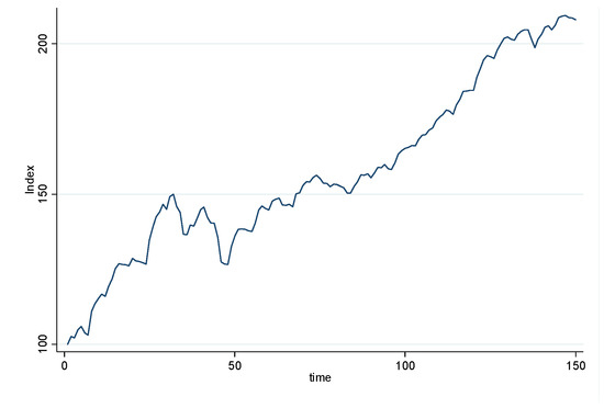
Figure 1.
Stockholm housing market. Note: The apartment price index. The Stockholm housing market and segments of the market (the x-axis is the measuring price index and the y-axis is the measuring time).
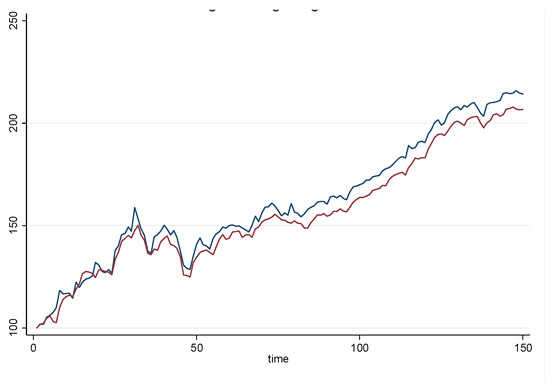
Figure 2.
Age segments. Note: The apartment price index. The Stockholm housing market and segments of the market (the x-axis is the measuring price index and the y-axis is the measuring time). The red line is equal newer apartment and the blue is equal older apartments.
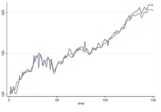
Figure 3.
Geography segments. Note: The apartment price index. The Stockholm housing market and segments of the market (the x-axis is the measuring price index and the y-axis is the measuring time). The red line is equal inner city and the blue is equal outer city.
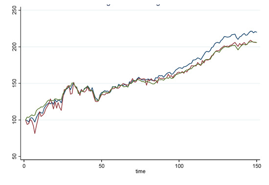
Figure 4.
Size segments. Note: The apartment price index. The Stockholm housing market and segments of the market (the x-axis is the measuring price index and the y-axis is the measuring time). The red line is equal one-room apartments, the blue is equal 2–3 room apartments and the green line equal large apartments.
Figure 1 clearly shows that the transaction price in the housing market in the Stockholm area has risen over the past few decades in general, up to an index value of 208 in June 2017 from 100 in January 2005. This means that the price for an apartment in 2017 was more than twice as expensive as it was in 2005. However, the price index also demonstrates that the price did not only rise. After the first peak at the index of 150 in August 2007, the price rapidly dropped and eventually reached 128 in November 2008, which can be attributed to the impact from the financial crisis starting in the USA in early 2008. During the period from the middle of 2006 to the end of 2009, the fluctuation of the transaction price in the Stockholm market showed an unstable market for apartments. That led to an increased risk when compared to the time after the end of 2011 when the prices rose consistently. However, the drop in the Stockholm apartment market is not comparable to some of the metropolitan regions in Europe and elsewhere.
Over the analyzed time period, the one-room apartment price index was generally higher than the total index for the same time frame, which probably means that the demand for one-room apartments can be considered to be higher when compared to the other types. Compared with other room types of apartments in Stockholm, the price index fluctuated for apartments with four or more rooms, which were more volatile most of the time and also faced a dramatic drop starting from early 2015.
Both apartment price indexes in the inner-city and suburbs of Stockholm were in line with the total index roughly from the period of early 2007 to mid-2011. However, the price development in the suburbs showed a lower price development when compared with the overall apartment market before 2007 and higher transaction prices after 2011. This could demonstrate that people may have switched preferences from previously buying apartments near central Stockholm to a tendency of nowadays moving out from central Stockholm. This could be a consequence of the fact that apartment prices in the inner-city are too expensive, so the demand has been pressed out to the suburbs.
The index of apartments that were older than 15 years was highly correlated with the total index during this period, which showed a good stability of transaction in this segment. Newer apartments had a higher volatility in prices as expected, as prices grew higher, especially during the early period, the sale prices were generally lower than the average market according to the index comparison shown above.
To summarize, most of the housing market segments have had more or less the same rapid apartment price development over the studied period. In general, the housing market in Stockholm faced a rather unstable period during the global financial crisis from early 2008 and then started to gradually increase afterward in terms of the transaction price. The most recent number has pointed out that the price is higher than twice its price in 2005. However, the volatility in the series differs. Some of the housing market segments exhibit more risk in the form of higher volatility and some other segments have had less risk. We will thoroughly analyze the price indices in the next section.
4.3. Beta Modeling
We estimated seven different beta models where we related the return on each segment of the housing market to the overall housing market. First, the descriptive statistics for each return series are presented in Table 3. The return series was derived from the apartment price indices by calculating the log return. The descriptive statistics for each return series were the following measures: average, standard deviation, kurtosis, skewness, and Dickey–Fuller test for non-stationarity together with the Durbin–Watson test for autocorrelation as well as an ARCH-LM test for heteroscedasticity in the return series.
Table 3.
The descriptive statistics: prices indices data.
We concluded that the average monthly returns were almost of the same magnitude, however, the variation measured with the standard deviation showed that variation in volatility was high. The volatility was higher in the older apartments segment, in the suburbs, and in larger apartments. None of the series were normally distributed. A close to normal distribution could be found in the newer apartment segment and in the suburbs. The distribution concerning older apartments was highly skewed to the right. All series peaked more than what could be expected when compared to a normal distribution. ARCH-LM tests showed if there was any heteroscedasticity over time in the return series, that is, if the volatility changed over time. The hypothesis about heteroscedasticity was rejected in the overall housing market and in the newer and older apartment segments as well as in the segment for one-room apartments. The Durbin–Watson test tests the hypothesis about the presence of serial correlation (or temporal autocorrelation). A value around two indicates that there is no serial correlation. Almost all series showed the presence of serial correlation. The Dickey–Fuller test is a test of stationarity. All the statistics in the table indicated that all series were stationary.
The model was first estimated using OLS and then tested for serial correlation. In all models, the serial correlation was present. As a remedy to the problem, we utilized the Cochrane–Orcutt regression technique. All t-values were based on White’s heteroscedasticity robust estimates (White 1980). Table 4 presents the results from these estimations.
Table 4.
The beta-analysis (Cochrane–Orcutt regression).
The overall goodness-of-fit showed a substantial variation among the eight different segments of the housing market. The variation in R2 ranged from 0.33 to 0.95. In the beta-model, the R-squared measures how closely each change in the price of a housing segment correlated to a benchmark, that is, the overall housing market. A low R-square value may indicate that the estimated beta values are less reliable. There is a risk of potential omitted variable bias in our estimates. One way to remedy this problem would be to also include social-economic variables in the model. However, this was not done in the present research. The measurements indicated that the market risk was very high in the new apartment, apartments in the inner-city, and one-room apartment segments. All these sub-markets followed the general trends in the overall market. However, segment specific risk was especially identified in the segments of the suburbs and 2–3 room apartments. All models exhibited serial correlation; therefore, the Cochrane–Orcutt approach was applied. After the transformation, all temporal autocorrelation was reduced to acceptable levels.
The beta model related the log returns for each segment against the return of the overall market. The average integral risk in the housing market of Stockholm was set to one, so any other beta in different types of housing segment could be compared with one. If it was more than 1, it meant that the price in this type of housing segment was more volatile than the overall market, thus bigger risks existed.
The beta also contained economical and quantified implications. For example, in the room size segment, the beta for one room, 2–3 rooms, and four or more rooms were 0.822, 0.983, and 1.328, respectively. It indicated that if the transaction price of the total market went up by 1%, the prices in these three kinds of apartments would be 0.822%, 0.983%, and 1.328%, respectively. This is a very important benchmark for later analysis in AHP methods for the suggestion of a risk-reduced portfolio proposal. The beta results regarding the correlation between the total market and apartment size segment had a relatively good accuracy. All estimates were statistically significantly different from zero. However, a more relevant hypothesis was to test whether the beta values were significantly different from one. Here, we noticed that the estimate concerning four rooms or more was not statistically different from one.
The beta coefficients concerning the geographical segmentation suggested that both markets had less risk than the overall market. However, only the estimate concerning the inner-city was statistically different from one. That is, the inner-city segment exhibited a lower risk than the overall housing market and the suburbs exhibited the same risk as the overall market. Concerning the age segmentation, we can conclude that none of the two estimates were statistically significantly different from one, indicating that both age groups exhibited the same risk.
4.4. Analytic Hierarchy Process Modeling
The first step in analytic hierarchy process modeling is to construct a hierarchy structure. Since three impact factors (geography, apartment size, and age) were chosen, the hierarchy was constructed based on this. Figure 5 depicts the structure of AHP for the different housing market segments.
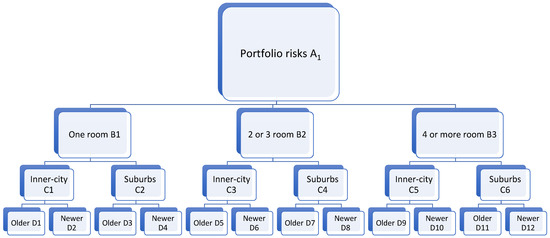
Figure 5.
The structure of AHP for different housing segments in Stockholm.
Each impact factor was different. For example, D1 represents apartments that were older than 15 years, located in the inner-city, and had one room; D5 represents apartments that were older, located in the inner-city but had two or three rooms. So, D1 and D5 were actually different factors. Since there were 21 different impact factors, there were 21 different indexes created for AHP. For example, the index of B1 was the index for apartments that had one room while the index of D1 was the index for apartments that had one room, that were located in the inner-city, and that were older than 15 years. The order from higher level to lower level could be changed, which means, for example, that the B level could present a distance factor or age factor, and the D level could also present the room size factor. This order of the structure is just an example for constructing a risk-reduced portfolio in housing apartments.
Since there were 21 different indexes constructed for the AHP when applying the same beta model, 21 different betas could also be carried out. Together with different hierarchies in the model, the beta matrices were created, which were used for the judgment matrices.
The first step was to determine the risks of the different housing segments in a different hierarchy if the market price increased by 1%. As the beta matrix shows the risk connection between the upper level and lower level in the AHP model, it was easy to estimate how many percentages of the price in each housing segment in a different hierarchy would increase if the market price increased by 1%. Table 5 presents the results of how much the price would appreciate each housing market segment if the overall housing price increased by 1%.
Table 5.
How much each segment would increase if the overall market price increased by 1.
According to the AHP model structure, if the market price increased by 1%, B1 would increase by 0.82%, which equaled its beta; and if B1 increased by 1%, C1 would increase by 0.75%, which equaled its beta. Hence, this means that if the market price increased by 1%, C1 would increase by 0.82 × 0.75 = 0.62%, which was the same number as shown above for C1. Following this principle, the direct risks at different levels to the market price could be carried out as in the table above.
In the next step, we calculated the risk-reduced portfolio weight according to AHP. As the weight sets in each hierarchy and betas from each lower level to higher level are given, the risk-reduced portfolio was created following the suggested weight sets from each factor level. The advantage of this portfolio is that the overall risks can be equally distributed from a higher level down to a lower level, which in turn, lessens the risks of the portfolio. A risk-reduced portfolio allows the market risk to be equally distributed into the lower level and makes the total portfolio less risky.
To obtain the risk-reduced portfolio weight in AHP, we needed to calculate the judgment matrices and weight set in the B, C, and D levels. Since the beta values in each hierarchy are already known, which presents the relationship between every lower impact factor to the upper impact factors, it is easy to reconstruct the relationship between every two factors in the same level. For example, in the beta values of A–B, if the A level increases by 1%, B1, B2, and B3 would increase to 0.82%, 0.98%, and 1.33%, respectively. This also showed a relationship between B1, B2, and B3 themselves when compared with each other. If “less risky” is taken as a higher score, the judgment matrices can be created by having each beta of an impact factor divide one another on the same level.
The judgment matrix in the B level:
Note: *: 1.20 = 0.98 (beta of B2)/0.82 (beta of B1), this means, in a way, that the B1 factor is 1.2 times more important than the B2 factor based on the principle that the less risky factor (smaller beta) scores are higher than those with the bigger risk. **: Following the same principle, 1.62 = 1.33/0.82; this way covers every number in the matrix and so on.
The judgment matrix in the C level:
The judgment matrix in the D level:
After the judgment matrices, the weight sets stand for how many percentages of the investment are suggested for the allocation between the sub-markets in, for example, the mortgage portfolio, to reduce the overall investing risks. Weight sets can be calculated in the AHP principle and are shown in Table 6.
Table 6.
The illustration of the weight set calculation for the B level.
Since the consistency test is necessary only when the number of factors in the same level is more than two, this means that only the judgment matrix in the B level needs examining. The result is as follows:
Since the CR is smaller than 0.1, this result passes the consistency test so the weight sets can be used for a risk-controlled portfolio.
Following the same principle, it is easy to calculate the weight sets for the C and D levels as shown in Table 7 and Table 8:
Table 7.
The weight set calculation for the C level.
Table 8.
The weight set calculation for the D level.
Table 9 presents all of the optimal weights and risk weights. The overall market risk was equal to one. The interpretation of the weight set was, for example in the B level, the suggested portfolio that would be invested, containing 41% of one-room apartments, 34% of two or three room apartments, and 25% of four or more room apartments in Stockholm, Sweden.
Table 9.
The optimal weight sets for the B, C, and D levels.
To summarize, this means that this is the best percentage of each segment factor in the portfolio that takes equal risk distribution into the next level. The total risk of the portfolio would be around 1.00, 0.73, and 0.64 for the B, C, and D levels, respectively, when compared with the market. Hence, level D minimizes the portfolio risk. It is not enough to diversify by only apartment size and space, the age of the property is also needed in the diversification.
4.5. Evaluation
The evaluation was carried out by comparing the Stockholm house price index with an index using optimal weight. In order to evaluate the proposed method, we used measures such as the average, standard deviation, kurtosis, and skewness on the monthly return series. The value-at-risk (VaR) was also utilized as an alternative measure of diversification benefit. Table 10 presents the descriptive statistics.
Table 10.
The evaluation of the results.
The results showed that with the optimal weight, the average return was higher, that is, the appreciation of the houses in the lenders’ portfolio increased more over time at the same time that the risk/volatility was lower (lower standard deviation). It is also interesting to note that the skewness of the return series was very different. The optimal weight (AHP-D) return series was skewed to the right, that is, the right tail of the distribution was long relative to the left tail. Both the AHD-C and MPT series were skewed to the left. The VaR at one month for a position on the Stockholm index was −2.6% at the 95% confidence level when compared to AHP-D at −3.4%. However, the difference was not statistically different at a 95% significance level.
5. Conclusions
Apartment size is usually seen as a very important impact factor in apartment sales, therefore, analyzing the data from 2005 to early 2017 in this paper showed a relatively accurate volatility of each size segment in terms of the transaction price. By setting up hedonic and beta modeling, the apartment pricing indexes and the relationship of each segment towards the overall market could be constructed. From the data analysis, a conclusion could be drawn that apartments that had four or more rooms in Stockholm had the most volatility when compared with other size type apartments, which also means that the investments put in this segment contained a higher risk.
Stockholm, Sweden, is often regarded as a city with a shortage of accommodation nowadays in the city center, which the data analysis also indicated. From both the results of the hedonic and beta modeling, it was shown that, interestingly, households had a tendency to purchase apartments in the city center from 2005 to 2007 that shifted to the urban area after 2011. Meanwhile, the two location segments were highly in line with the total market. This implies that nowadays, accommodation in the Stockholm city center is becoming more and more limited, so it has pushed people to think about buying the apartments further from city center, which probably means that today, apartments further away from the city center have more investment value than ones closer to the center.
Without any doubt, the results have shown that the newer apartments (less than 15 years) have a higher pricing volatility than older apartments, which means that they contain more investment risk than the other. However, this phenomenon has cooled down a bit in recent years since apartments in those two age segments are more and more in line with the total market for the last few years in Stockholm.
After examining the correlation between different housing segments and the overall market, it is interesting, going further, to determine what a reduced-risk apartment investment portfolio should be, and how much of each housing segment should be contained in this portfolio. By applying beta modeling and AHP methods from systems engineering, the weight set of each segment can be carried out, which represents how much investment funding from each segment should be put into the portfolio to reduce the risks as much as possible.
In this paper, the housing segments of apartment size, age, and location, in general, are chosen and three hierarchies were created. The calculation results showed that for a given investment portfolio for apartments, it is wise to put the most funds into apartments that have one room, are older, and are located in the inner-city, followed by apartments that have one room, are older, but further from the city center. This portfolio arrangement can reduce the bundled total risk to a level that is lower than the market risk by allowing the risks to be equally distributed into the next hierarchy level.
What are the policy implications for the lender? Typically, the lender analysis will be of both the borrower and the object, the apartment. The focus has been on the borrower. The lender looks at the loan-to-value ratio, income in relation to debt service, and of course, the credit history of the borrower. The main objective has been to reduce the default probability. A lender to a real estate developer typically focuses more on the object, for example, the net operating income, vacancy rates, and break-even levels, than the borrower. What we proposed in this paper was that the mortgage lender could also benefit by more carefully analyzing the object and specifically the housing market segment more carefully. By controlling borrower characteristics, the risk for the lender can be reduced by utilizing a strategy considering the distribution of mortgages in different housing market segments. Even within a metropolitan housing market, as we investigated in this paper, diversifying does entail potential benefits (higher return and less risk). The benefits are probably even higher if inter-regional diversification is considered.
Author Contributions
Conceptualization, M.W. and J.Z.; Methodology, M.W. and J.Z.; Software, M.W.; Validation, M.W. and J.Z.; Formal Analysis, M.W. and J.Z.; Investigation, M.W. and J.Z.; Resources, M.W.; Data Curation, M.W.; Writing—Original Draft Preparation, M.W. and J.Z.; Writing—Review & Editing, M.W. and J.Z.; Visualization, M.W.; Supervision, M.W.
Funding
This research received no external funding.
Conflicts of Interest
The authors declare no conflict of interest.
References
- Afonso, António, and Ricardo M. Sousa. 2011. The macroeconomic effects of fiscal policy. Applied Economics 44: 4439–54. [Google Scholar] [CrossRef]
- Agnello, Luca, and Ludger Schuknecht. 2011. Booms and busts in housing markets: Determinants and implications. Journal of Housing Economics 20: 171–90. [Google Scholar] [CrossRef]
- Ayan, Ebubekir, and H. Cenk Erkin. 2014. Hedonic Modeling for a Growing Housing Market: Valuation of Apartments in Complexes. International Journal of Economics and Finance 6: 188. [Google Scholar] [CrossRef]
- Baltas, George, and Jonathan Freeman. 2001. Hedonic Price Methods and the Structure of High-Technology Industrial Markets: An Empirical Analysis. Industrial Marketing Management 30: 599–607. [Google Scholar] [CrossRef]
- Baudry, Marc, and Masha Maslianskaia-Pautrel. 2015. Revisiting the hedonic price method in the presence of market segmentation. Environmental Economics and Policy Studies 18: 1–29. [Google Scholar] [CrossRef]
- Bender, Andre, Allan Din, Philippe Favarger, Martin Hoesli, and Janne Laakso. 1997. An analysis of Perception Concerning the Environmental Quality of Housing in Geneva. Urban Studies 34: 503–13. [Google Scholar] [CrossRef]
- Beracha, Eli, and Hilla Skiba. 2011. Findings from a cross-sectional housing risk-factor model. Journal of Real Estate Financial Economics 47: 289–309. [Google Scholar] [CrossRef]
- Berggren, Björn, Andreas Fili, and Mats Håkan Wilhelmsson. 2017. Does the increase in house prices influence the creation nof business startups? The case of Sweden. Region 4: 1–16. [Google Scholar] [CrossRef]
- Bernard, Carole, Ludger Rüschendorf, Steven Vanduffel, and Jing Yao. 2017. How robust is the value-at-risk of credit risk portfolios? The European Journal of Finance 23: 507–34. [Google Scholar] [CrossRef]
- Bhushan, Navneet, and Kanwal Rai. 2004. Strategic Decision Making: Applying the Analytic Hierarchy Process. London: Springer. ISBN 1-85233-756-7. [Google Scholar]
- Zhu, Bin, and Zeshui Xu. 2014. Analytic hierarchy process-hesitant group decision making. European Journal of Operational Research 239: 794–801. [Google Scholar] [CrossRef]
- Boffelli, Simona, and Giovanni Urga. 2016. Financial Econometrics Using STATA. College Station: Stata Press. [Google Scholar]
- Bollen, Bernard, and Philip Gharghori. 2015. How is β related to asset returns? Applied Economics 48: 1925–35. [Google Scholar] [CrossRef]
- Bourassa, Steven C., Foort Hamelink, Martin Hoesli, and Bryan D. MacGregor. 1999. Defining Housing Submarkets. Journal of Housing Economics 8: 160–83. [Google Scholar] [CrossRef]
- Brasington, David M., and Diane Hite. 2005. Demand for environmental quality: A spatial hedonic analysis. Regional Science and Urban Economics 35: 57–82. [Google Scholar] [CrossRef]
- Brown, Scott R. 2016. The Influence of Homebuyer Education on Default and Foreclosure Risk: A Natural Experiment. Journal of Policy Analysis and Management 35: 145–72. [Google Scholar] [CrossRef]
- Campbell, John Y., and Tuomo Vuolteenaho. 2004. Bad beta, good beta. American Economic Review 94: 1249–75. [Google Scholar] [CrossRef]
- Cannon, Susanne, Norman G. Miller, and Gurupdesh S. Pandher. 2006. Risk and Return in the U.S. Housing Market: A Cross-Sectional Asset-Pricing Approach. Real Estate Economics 34: 519–52. [Google Scholar] [CrossRef]
- Cerutti, Eugenio, Jihad Dagher, and Giovanni Dell’Ariccia. 2017. Housing finance and real-estate booms: A cross-country perspective. Journal of Housing Economics 38: 1–13. [Google Scholar] [CrossRef]
- Chatterjee, Satyajit, and Burcu Eyigungor. 2015. A quantitative analysis of the US housing and mortgage markets and the foreclosure crisis. Review of Economic Dynamics 18: 165–84. [Google Scholar] [CrossRef]
- Clauretie, Terrence. 1988. Regional Economic Diversification and Residential Mortgage Default Risk. Journal of Real Estate Research 3: 87–97. [Google Scholar]
- Corgel, John B., and Gerald D. Gay. 1987. Local Economic Base, Geographic Diversification, and Risk Management of Mortgage Portfolios. AREUEA Journal 15: 256–67. [Google Scholar] [CrossRef]
- Cotter, John, Stuart Gabriel, and Richard Roll. 2015. Can Housing Risk be Diverfied? A Cautionary Tale from the Housing Boom and Bust. The Review of Financial Studies 28: 913–36. [Google Scholar] [CrossRef]
- Crowe, Christopher, Giovanni Dell’Ariccia, Deniz Igan, and Pau Rabanal. 2013. How to deal with real estate booms: Lessons from country experiences. Journal of Financial Stability 9: 300–19. [Google Scholar] [CrossRef]
- Dey, Prasanta Kumar. 2010. Managing project risk using combined analytic hierarchy process and risk map. Applied Soft Computing 10: 990–1000. [Google Scholar] [CrossRef]
- Domian, Dale, Rob Wolf, and Hsiao-Fen Yang. 2015. An assessment of the risk and return of residential real estate. Managerial Finance 41: 591–99. [Google Scholar] [CrossRef]
- Donner, Herman, Han-Suck Song, and Mats Wilhelmsson. 2016. Forced sales and their impact on real estate prices. Journal of Housing Economics 34: 60–68. [Google Scholar] [CrossRef]
- Duffie, Darrell, and Jun Pan. 1997. An overview of Value at Risk. Journal of Derivatives 4: 7–49. [Google Scholar] [CrossRef]
- Fama, Eugene F. 1976. Foundations of Finance: Portfolio Decisions and Securities Prices. New York: Basic Books. [Google Scholar]
- Favilukis, Jack, Sydney C. Ludvigson, and Stijn Van Nieuwerburgh. 2017. The macroeconomic effects of housing wealth, housing finance, and limited risk sharing in general equilibrium. Journal of Political Economy 125: 140–223. [Google Scholar] [CrossRef]
- Ferreira, Eva, Javier Gil-Bazo, and Susan Orbe. 2011. Conditional beta pricing models: A nonparametric approach. Journal of Banking & Finance 35: 3362–82. [Google Scholar]
- Firstenberg, Paul M., Stephen A. Ross, and Randall C. Zisler. 1988. Real estate: The whole story. Journal of Portfolio Management 14: 22–34. [Google Scholar] [CrossRef]
- Forman, Ernest H., and Saul I. Gass. 2001. The Analytic Hierarchy Process: An Exposition. Operations Research 49: 469–86. [Google Scholar] [CrossRef]
- Fouque, Jean-Pierre, and Adam P. Tashman. 2012. Option pricing under a stressed-beta model. Annals of Finance 8: 183–203. [Google Scholar] [CrossRef]
- Goodman, Allen C., and Thomas G. Thibodeau. 2003. Housing market segmentation and hedonic prediction accuracy. Journal of Housing Economics 12: 181–201. [Google Scholar] [CrossRef]
- Ilmanen, Antti. 2014. Expected Returns: An Investor’s Guide to Harvesting Market Rewards. Quantitative Finance 14: 581–82. [Google Scholar]
- Huang, Xin, Hao Zhou, and Haibin Zhu. 2012. Assessing the systemic risk of a heterogeneous portfolio of banks during the recent financial crisis. Journal of Financial Stability 8: 193–205. [Google Scholar] [CrossRef]
- Huffman, Forrest E. 2003. Corporate real estate risk management and assessment. Journal of Corporate Real Estate 5: 31–41. [Google Scholar] [CrossRef]
- Ibbotson, Roger G., and Laurence B. Siegel. 1984. Real estate returns: A comparison with other investments. Real Estate Economics 12: 219–42. [Google Scholar] [CrossRef]
- Jones, Colin, Chris Leishman, and Craig Watkins. 2004. Intra-Urban migration and housing submarkets: Theory and evidence. Housing Studies 19: 269–83. [Google Scholar] [CrossRef]
- Joro, Tarja, and Paul Na. 2006. Portfolio performance evaluation in a mean-variance-skewness framework. European Journal of Operational Research 175: 446–61. [Google Scholar] [CrossRef]
- Hyun, Ki-Chang, Sangyoon Min, Hangseok Choi, Jeongjun Park, and In-Mo Lee. 2015. Risk analysis using fault-tree analysis (FTA) and analytic hierarchy process (AHP) applicable to shield TBM tunnels. Tunnelling and Underground Space Technology 49: 121–29. [Google Scholar] [CrossRef]
- Lintner, John. 1975. The Valuation of Risk Assets and the Selection of Risky Investments in Stock Portfolios and Capital Budgets. Stochastic Optimization Models in Finance 51: 220–21. [Google Scholar] [CrossRef]
- Malpezzi, Stephen. 2003. Hedonic pricing models: A selective and applied review. In Housing Economics and Public Policy. Oxford: Blackwell Publishing. [Google Scholar]
- Markowitz, Harry. 1952. Portfolio selection. Journal of Finance 7: 77–91. [Google Scholar]
- Monson, Matt. 2009. Valuation using hedonic pricing models. Cornell Real Estate Review 7: 10. [Google Scholar]
- Ogden, William, Nanda Rangan, and Thomas Stanley. 1989. Risk Reduction in S&L Mortgage Loan Portfolios Through Geographic Diversification. Journal of Financial Service Research 2: 39–48. [Google Scholar]
- Ortas, Eduardo, Manuel Salvador, and Jose Moneva. 2014. Improved beta modeling and forecasting: An unobserved component approach with conditional heteroscedastic disturbances. The North American Journal of Economics and Finance 31: 27–51. [Google Scholar] [CrossRef]
- Pu, Ming, Gang-Zhi Fan, and Chunsheng Ban. 2016. The pricing of mortgage insurance premiums under systematic and idiosyncratic Shocks. Journal of Risk and Insurance 83: 447–74. [Google Scholar] [CrossRef]
- Reeves, Jonathan J., and Haifeng Wu. 2013. Constant versus Time-Varying Beta Models: Further Forecast Evaluation. Journal of Forecasting 32: 256–66. [Google Scholar] [CrossRef]
- Rosenberg, Barr, and James Guy. 1995. Prediction of Beta from Investment Fundamentals. Financial Analysts Journal 51: 101–12. [Google Scholar] [CrossRef]
- Saaty, Thomas L. 1980. The Analytical Hierarchy Process. New York: McGraw-Hill. [Google Scholar]
- Saaty, Thomas L. 2008. Decision Making for Leaders: The Analytic Hierarchy Process for Decisions in a Complex World. Pittsburgh. Pittsburgh: RWS Publications. ISBN 0-9620317-8-X. [Google Scholar]
- Saaty, Thomas L., and Kirti Peniwati. 2008. Group Decision Making: Drawing out and Reconciling Differences. Pittsburgh: RWS Publications. ISBN 978-1-888603-08-8. [Google Scholar]
- Saita, Francesco. 2008. Value at Risk and Bank Capital Management. Risk Adjustment Performances, Capital Management and Capital Allocation Decision Making. Burlington. Waltham: Academic Press publications, Elsevier. [Google Scholar]
- Saracoglu, Burak Omer. 2013. Selecting industrial investment locations in master plans of countries. European Journal. of Industrial Engineering 7: 416–41. [Google Scholar] [CrossRef]
- Scholes, Myron, and Joseph Williams. 1977. Estimating betas from nonsynchronous data. Journal of Financial Economics 5: 309–27. [Google Scholar] [CrossRef]
- Sharpe, William F. 1964. Capital asset prices: A theory of market equilibrium under conditions of risk. The Journal of Finance 19: 425–42. [Google Scholar]
- Shiller, Robert J. 2014. Speculative Asset Prices. The American Economic Review 104: 1486–517. [Google Scholar] [CrossRef]
- Song, Han-Suck, and Mats Wilhelmsson. 2010. Improved price index for condominiums. Journal of Property Research 27: 39–60. [Google Scholar] [CrossRef]
- Srinivasan, Venkat C. 1994. Using the analytical hierarchy process in house selection. Journal of Real Estate Finance and Economics 9: 69–85. [Google Scholar]
- Tofallis, Chris. 2008. Investment volatility: A critique of standard beta estimation and a simple way forward. European Journal of Operational Research 187: 1358–67. [Google Scholar] [CrossRef]
- White, Halbert. 1980. A Heteroscedasticity-Consistent Covariance Matrix Estimator and a Direct Test for Heteroskedasticity. Econometrica 40: 817–38. [Google Scholar] [CrossRef]
- Wilhelmsson, Mats. 2002. Spatial models in real estate economics. Housing, Theory and Society 19: 92–101. [Google Scholar] [CrossRef]
- Wilhelmsson, Mats. 2004. A method to derive housing sub-markets and reduce spatial dependency. Property Management 22: 276–88. [Google Scholar] [CrossRef]
- Wu, Jing, Yongheng Deng, and Hongyu Liu. 2014. House price index construction in the nascent housing market: The case of China. The Journal of Real Estate Finance and Economics 48: 522–45. [Google Scholar] [CrossRef]
- Zhao, Xiaogang, Yi Zhou, and Jianyu Zhao. 2011. Fire safety assessment in oil depot based on Comprehensive Grey Relational Analysis. Paper presented at Reliability, Maintainability and Safety (ICRMS), 2011 9th International Conference on, Guiyang, China, June 12. [Google Scholar]
- Zhao, Xiaogang, Yi Zhou, and Jianyu Zhao. 2013a. Application of Fuzzy Analytic Hierarchy Process in Selection of Electrical Heat Tracing Elements in Oil Pipelines. Applied Mechanics and Materials 367: 452–56. [Google Scholar] [CrossRef]
- Zhao, Jian Yu, Yi Zhou, and Xiao Yang Cai. 2013b. Selection of Engineering Management University Internship Projects Based on Fuzzy Analytic Hierarchy Process. Advanced Materials Research 787: 1002–5. [Google Scholar] [CrossRef]
- Zheng, Xiao, and Shui Tai Xu. 2010. The Risk Assessment Research on Real Estate Projects in View of Fuzzy-Synthetical Evaluation. Applied Mechanics and Materials 29: 2455–61. [Google Scholar] [CrossRef]
- Zietz, Joachim, Emily Norman Zietz, and G. Stacy Sirmans. 2008. Determinants of house prices: A quantile regression approach. Journal of Real Estate Finance and Economics 37: 317–33. [Google Scholar] [CrossRef]
- Zopounidis, Constantin. 1999. Multicriteria decision aid in financial management. European Journal of Operational Research 119: 404–15. [Google Scholar] [CrossRef]
© 2018 by the authors. Licensee MDPI, Basel, Switzerland. This article is an open access article distributed under the terms and conditions of the Creative Commons Attribution (CC BY) license (http://creativecommons.org/licenses/by/4.0/).