Abstract
In this paper, we compare the transmission of a conventional monetary policy shock with that of an unexpected decrease in the term spread, which mirrors quantitative easing. Employing a time-varying vector autoregression with stochastic volatility, our results are two-fold: First, the spread shock works mainly through a boost to consumer wealth growth, while a conventional monetary policy shock affects real output growth via a broad credit/bank lending channel. Second, both shocks exhibit a distinct pattern over our sample period. More specifically, we find small output effects of a conventional monetary policy shock during the period of the global financial crisis and stronger effects in its aftermath. This might imply that when the central bank has left the policy rate unaltered for an extended period of time, a policy surprise might boost output particularly strongly. By contrast, the spread shock has affected output growth most strongly during the period of the global financial crisis and less so thereafter. This might point to diminishing effects of large-scale asset purchase programs.
JEL Classification:
C32; E52; E32
1. Introduction
With the onset of the global financial crisis, the U.S. Federal Reserve (Fed) began to lower interest rates to stimulate the economy. Since December 2008, however, the federal funds rate (FFR) is effectively zero, leaving no room for conventional monetary policy to further enhance economic growth. Against the backdrop of lackluster economic conditions and the perceived risks of deflation at that time, the U.S. Fed decided to engage in an “unconventional” monetary policy, which took mostly the form of asset purchases from the private banking and non-banking sector. After three large-scale asset purchase programs (LSAPs), assets on the central bank’s balance sheet more than quadrupled since 2007 to about 4500 billion U.S. dollars in February 2015.
While a large body of empirical literature has hitherto investigated how conventional U.S. monetary policy affects the real economy, there is less empirical research on the transmission of quantitative easing (QE). QE implies switching from interest rate targeting steered via reserve management to targeting the quantity of reserves (Fawley and Juvenal 2012). In the USA, the Fed did so by buying longer term securities either issued by the U.S. government or guaranteed by government-sponsored agencies. This should directly put downward pressure on long-term yields in these markets. In addition, financing conditions will ease more generally, since investors selling to the Fed reinvest those proceeds to buy other longer term securities such as corporate bonds and other privately-issued securities (portfolio re-balancing, Joyce et al. 2012). On the back of increased equity prices and heightened loan demand, both private sector wealth and asset growth in the banking sector should tick up, leading to an increase in aggregate demand.
The strength of these transmission channels is likely to depend on the current economic environment. In fact, and considering the transmission of conventional monetary policy, several authors have suggested that the transmission mechanism has changed over time; see, e.g., (Boivin and Giannoni 2006; Boivin et al. 2010; Breitfuß et al. 2018). In a recent contribution, Kastner et al. (2018) found empirical evidence for a change in transmission related to inflation, namely a considerable price puzzle (i.e., an increase in the price level after a monetary policy contraction) in the 1960s, which starts disappearing in the early 1980s. Miranda-Agrippino and Ricco (2017) showed for the USA that price and output puzzles vanish once a robust identification strategy and a rich information set are considered. They also acknowledged that the emergence of such puzzles can indeed depend on the sample period under study. Looking at more recent data, the global financial crisis was a severe rupture of the financial system and could have potentially changed the way monetary policy was conducted. Arguments why a monetary policy shock might have smaller effects during recessions associated with financial crises such as the one in 2008/2009 include balance sheet adjustments and deleveraging in the private sector, which typically takes place after economic boom phases that predate financial crises (Bech et al. 2014). Furthermore, heightened uncertainty might weigh on the business climate and impede investment growth. The works in Aastveit et al. (2017) and Hubrich and Tetlow (2015) investigated monetary policy in times of financial stress or heightened uncertainty and found smaller effects in these periods for the USA. The work in Tenreyro and Thwaites (2016) more generally found that U.S. monetary policy is less effective during recessions. Whether these arguments carry over to unconventional monetary policy is less researched. Recent work actually suggests the opposite. For example, Engen et al. (2015) emphasized the role of quantitative easing in underpinning the commitment of the Fed to be accommodative for a longer period. This signaling channel is more effective when financial markets are impaired and economic conditions characterized by high uncertainty. This reasoning ascribes quantitative easing the greatest effectiveness during the onset of a crisis, contrasting the empirical work on the effectiveness of conventional monetary policy during financial crises. In a recent paper, Wu (2014) corroborated this result attesting the latest asset purchase programs having a smaller effect than the earlier ones.
In this paper, we address these questions within a coherent econometric framework. More specifically, and to cover a broad range of potential transmission channels, we propose a simple Bayesian estimation framework that handles medium- to large-scale models and that allows for drifting parameters and time-varying variances and covariances. Accounting for time variation and including a rich information set enhance the model to yield an appropriate representation of the underlying data. Moreover, since we assume that changes happen gradually, no further assumptions about the number of regimes such as in a Markov-switching framework have to be made. Akin to Baumeister and Benati (2013), we model the asset purchases of the U.S. Fed by assuming a compression of the yield curve. The transmission of the “spread shock” is compared with that of a conventional monetary policy shock.
Our main results can be summarized as follows: First, we find evidence that unconventional monetary policy works mainly via the wealth channel to spur aggregate demand. There is less evidence for the credit/bank lending channel. Second, conventional monetary policy works strongly through expanding assets and deposits of the banking sector, while the impact on consumer wealth growth is more modest. Last, for both shocks, we find a distinct pattern over our sample period. More specifically, we find small output effects of a conventional monetary policy shock during the period of the global financial crisis and stronger effects in its aftermath. This might imply that when the central bank has successfully committed the policy rate to a certain value, an unexpected deviation from that commitment might boost output growth particularly strongly. By contrast, the spread shock has affected output growth most strongly during the period of the global financial crisis, when the Fed launched its first asset purchase program, and less so thereafter. This might point to diminishing effects of large-scale asset purchase programs on real output growth.
2. Econometric Framework
In this section, we introduce the data, the econometric framework and the identification strategy to investigate the transmission of unconventional and conventional monetary policy. We use a novel approach to estimation based on the work by Lopes et al. (2013) that can handle medium- to large-scale time-varying vector autoregressions with stochastic volatility (TVP-SV-VAR).
2.1. Data
Our analysis is based on variables typically employed in monetary vector autoregressions and on a quarterly frequency. The time period we consider spans from 1984Q1 to 2015Q1, and the variables comprise real GDP growth (), consumer price inflation (), the federal funds rate () and the term spread (sp) defined as the yield on 10-year-government bonds minus the federal funds rate. In addition to these standard variables, we include several variables that should allow us to gauge the importance of different channels for monetary policy transmission. These are growth in net household and non-profit organizations’ wealth (), growth in commercial banks’ assets and deposits () and the net interest rate margin (nim) of large U.S. banks. Growth rates are calculated as log-differences and are thus in quarter-on-quarter terms.1
2.2. The TVP-SV-VAR Model with a Cholesky Structure
In what follows, we draw on a new approach to estimate a TVP-SV-VAR. This approach differs from standard estimation by recasting the VAR as a system of unrelated regressions and imposing a recursive structure on the model a priori.
We collect the data in an vector:
Now, we assume the individual elements of to be described by a set of equations, with the first equation given by:
and for :
where denotes a constant and are m-dimensional coefficient vectors associated with the lags of in each equation. The triangular structure is imposed on the contemporaneous coefficients. More specifically, the denote coefficients associated with the first elements of with for . Finally, is a normally distributed error with time-varying variance given by . Note that all coefficients in Equations (1)–(4) are allowed to vary over time.
We assume that evolves according to:
is a standard white noise error term with variance . Equation (5) implies that the parameters associated with the contemporaneous terms are following a random walk.
Let us define an -dimensional vector . Similarly to Equation (5), we assume that follows the subsequent law of motion:
with being a vector white noise error with the variance-covariance matrix equal to . Finally, the s follow:
where denotes the log-volatility, is the mean of the log-volatility and the autoregressive parameter. is the zero-mean error term with variance . Several studies have shown that it is important to allow for both changes in residual variances and parameters. Assuming constant error variances, while they are in fact time-varying, could lead to misleading parameter estimates of the VAR.2 Moreover, changes in the economic environment can affect how monetary policy transmits to the real economy. In other words, previous literature suggested that the volatility of economic shocks also tends to influence real activity (Bloom 2009; Fernández-Villaverde et al. 2011).
The reason why the log-volatility process is assumed to be stationary in contrast to the non-stationary state equation of the autoregressive parameters is mainly due to the fact that a random walk assumption for the log-volatility would imply that it is unbounded in the limit, hitting any lower or upper bound with probability one. In practice, however, the differences between a stationary and non-stationary state equation are negligible since the data are not really informative about the specific value of .3
The model given by Equations (1)–(4) can be recast in a more compact form by collecting all contemporaneous terms on the left-hand side:
where denotes an lower triangular matrix with diagonal and the typical non-unit/non-zero element given by . Here, we let be an m-dimensional unit vector. In what follows we collect free elements of in an vector . is an vector of constants, and denotes an dimensional coefficient matrix to be estimated. The m-dimensional error vector has zero mean and a diagonal time-varying variance-covariance matrix given by . Equation (8) resembles the structural TVP-SV-VAR model put forth in Primiceri (2005). The lower triangular nature of is closely related to a recursive identification scheme, which assumes a natural ordering of variables. In fact, we use the ordering as the variables appear in . However, note that we do not identify the shocks based on this Cholesky decomposition. Rather, we impose the triangular structure due to computational reasons only, while identification of the shocks will be based on sign restrictions discussed in Section 2.4. These are two isolated steps, and the a priori Cholesky decomposition does not interfere with identification based on sign restrictions, which re-weights orthogonalized errors (that we directly obtain from the estimation stage of the model) and selects those that fulfill the postulated sign restrictions. Our structural analysis will thus be unaffected by the triangular structure imposed on the model. For an excellent overview on sign restrictions, see Fry and Pagan (2011). In Section 3.5, we show that estimates based on a different ordering yield virtually the same impulse response functions.
In the absence of specific assumptions on , the model in Equation (8) is not identified. Thus, researchers usually estimate the reduced form imposing restrictions that originate from theory ex-post.4 The reduced form of the TVP-SV-VAR is given by:
with , and . The reduced form errors are normally distributed with the variance covariance matrix given by . It can easily be seen that the matrix establishes contemporaneous links between the variables in the system.
To emphasize the distinct features of our estimation strategy, it is worth mentioning how this model is traditionally estimated. Typically, one would start with the complete system of reduced form equations given in Equation (9) and obtain reduced form parameter estimates by employing Gibbs sampling coupled with a data augmentation scheme (Cogley et al. 2005; Primiceri 2005). This approach to estimation comes along with a significant computational burden. To be more precise, if as in our case, and the number of lags is set to , the algorithms outlined in Carter and Kohn (1994) and Frühwirth-Schnatter (1994) require the inversion of a variance-covariance matrix at each point in time. In our case, would be , rendering estimation with the traditional algorithms cumbersome.5
Following Lopes et al. (2013), we impose a Cholesky structure a priori, estimate the structural form in an equation-by-equation fashion and use the estimated coefficients to solve Equation (8) to finally obtain Equation (9). Using an equation-by-equation approach decreases the computational burden significantly, by first reducing the dimension of the matrices that have to be inverted. More specifically, while the inversion of a matrix requires operations using Gaussian elimination, we reduce this to , which is a marked gain as compared to full-system estimation. Second, and more importantly, equation-by-equation estimation can make full use of parallel computing. Recently, Carriero et al. (2015) suggested a related estimation strategy, which imposes a triangular structure on the errors rather than the contemporaneous coefficients related to the dependent variable. While this approach is invariant to the ordering of the variables, it prohibits parallel computing, and hence, computational gains are more limited.
2.3. Bayesian Inference
We use a Bayesian approach and impose tight priors on the variance-covariance structure in the various state equations, which describe the law of motion for the parameters.
General Prior Setup and Implementation
Following Primiceri (2005) and Cogley et al. (2005), we impose a normally distributed prior on the free elements of the initial state , which are collected in a vector and on :
where and are prior mean matrices and and are prior variance-covariance matrices. We follow common practice (Primiceri 2005) and use a training sample of quarters to scale the priors. We set the prior mean for and equal to the OLS estimate based on this training sample. The prior variance-covariance matrices are specified such that and , with and being the variances of the OLS estimator.6
The priors on the variance-covariances in the state Equations (5) and (6) are of the inverted Wishart form:
with denoting the variance-covariance matrix of . This matrix is block-diagonal with each block corresponding to the m equations of the system. The degree of freedom parameters are denoted by and , and the corresponding prior scaling matrices are labeled as and . In principle, we set and , with being a scalar parameter controlling the tightness on the propensity of to drift. We set after having experimented with a grid of different values. The results remain qualitatively unchanged as long as the prior is not set too loose, placing much prior mass on regions of the parameter space, which imply explosive behavior of the model. We use the same hyperparameters for the prior on , i.e., and with . Again, this choice is based on experimenting with a grid of values ruling out hyperparameter choices that imply excessively explosive behavior of the model.
Finally, we follow Kastner and Frühwirth-Schnatter (2013) and set and , implying a loose prior on the level of the log-volatility. The prior on is set such that much prior mass is centered on regions for close to unity, providing prior evidence for the non-stationary behavior of . Thus, we set and . For the non-conjugate Gamma prior on , we set equal to one. The Appendix contains a brief sketch of the Markov Chain Monte Carlo (MCMC) algorithm to estimate the model.
2.4. Structural Identification
To identify a U.S. monetary policy shock and a shock to the term spread, we use a set of sign restrictions put directly on the impulse responses.7 More specifically, we identify a “monetary policy” or “term spread” shock by singling out from a set of generated responses those that comply with our a priori reasoning about how the economy typically responds to either of the shocks. The restrictions refer to the directional movements of impulse responses on impact and are outlined in Table 1.

Table 1.
Identification via sign restrictions.
We look at two shocks related two monetary policy and three broad transmission channels.8 We assume that an expansionary conventional monetary policy shock works via an unexpected lowering of the short-term interest rate. The most direct way lower interest rates feed into the economy is via the “interest rate/investment” channel. The decrease in the policy rate lowers the user cost of capital, thereby spurring investment and real GDP growth (Ireland 2005). In addition, aggregate demand can also increase through a boost to “consumption wealth”, as advocated in Ludvigson et al. (2002). Following a monetary expansion, equity prices are likely to tick up since the price of debt instruments rises in parallel with the reduction of the short-term rate, making them less attractive for investors (Ireland 2005). This leads to an increase in consumer wealth, which might boost consumption spending and aggregate demand (Ludvigson et al. 2002).
The cut in short-term interest rates has also bearings on the financial side of the economy. We assume an increase in the term spread in response to a decrease of the policy rate. This can be motivated by an imperfect pass-through along the term structure, implying that long-term interest rates do not follow the decrease in short-term interest rates one-to-one (Baumeister and Benati 2013).9 Trailing the term spread, net interest rate margins of banks tend to increase (Adrian and Shin 2010). This affects asset and deposit growth of the banking sector along two dimensions. First, the decrease in the long-term rate (even if less pronounced than that of short-rates) makes taking a loan cheaper, implying that the demand for loans is strengthened by the policy-induced decrease of the short-term rate. This effect is amplified by an improvement of balance sheets of households and firms on the back of the policy-induced rise of asset prices, which increases the demand for loans by those that were previously excluded from access to credit (“balance-sheet channel”). Second and since net interest rate margins increase, generating new loans becomes more attractive for banks (compared to faring excessive reserves with the Fed). Thus, the supply for loans is stimulated as well. As a consequence, deposit growth is assumed to tick up. The newly-generated loans will increase deposits mechanically since for each newly-issued loan, the bank creates a deposit of the same amount. On top of that, the increase of reservable deposits created by the monetary expansion will reduce the amount of managed liabilities banks need to fund their loans. This might be passed on to their clients by lowering loan rates and increasing loan supply (Bernanke and Blinder 1988; Black et al. 2007). We summarize these developments under a broad “credit and bank lending channel”. Naturally, aggregate demand is positively affected by loan growth, which leads to more investment and consumption.
Second, we investigate a shock to the term spread. Since the purchases of longer term securities have significantly lowered longer term yields, as demonstrated, e.g., in Doh (2010), Gagnon et al. (2011), Krishnamurthy and Vissing-Jorgensen (2011) and Hamilton and Wu (2012), assuming a reduction of the term spread can be thought of as a way to model the effects of quantitative easing within a standard monetary VAR framework. In contrast to a conventional expansionary monetary policy shock, asset purchases by the central bank will trigger a decrease in the term spread. As with the monetary policy shock, a shock to the term spread will trigger an increase in equity prices since yields on debt securities decline. An increase in consumer wealth, coupled with eased finance conditions, should spur economic activity and inflation. That asset purchase programs had an effect on consumer confidence through signaling has been emphasized in Engen et al. (2015) and Wu (2014). While we can investigate the signaling channel implicitly by tracing the effectiveness of unconventional monetary policy through periods of different financial and economic conditions, we cannot model this transmission mechanism explicitly by including a suitable control variable. Looking at the financial side of the economy, the reduction of the term spread triggers a decrease in net interest margins of commercial banks: since the cost of funding (the short-term interest rate) is unaltered and tied to the zero lower bound, the revenues of lending (approximated by the long-term interest rate) decrease. As in Adrian and Shin (2010), this implies an inward shift of the supply curve of credit and is likely to contain new lending. This effect, however, might be offset by a stronger demand for lending, since lower long-term rates make it more attractive to take a loan. Since a priori, we do not know which of these effects is likely to dominate, we leave the signs on growth in bank assets unrestricted. Next and in line with the assumption about the monetary policy shock, we assume an initial increase in banks’ deposits. This increase is rather mechanical since the proceeds of the asset purchase will be deposited in the investors’ bank accounts, raising deposits of the banking sector, and might be rather short-lived, as pointed out in Butt et al. (2014).10
Last and to mimic the zero lower bound environment, we will hold the response of the short-term interest rate constant at zero for eight quarters (Baumeister and Benati 2013). Note that this is unrelated to identification of the shock, for which restrictions are only binding on impact. The Appendix provides further details on the technical implementation of the sign restrictions and the zero restriction on the short-term interest rate for the spread shock.
3. Empirical Results
In this section, we investigate the transmission of the monetary policy and the term spread shock, examine whether overall effects vary over time and establish that both shocks mattered historically in determining fluctuations in the time series considered in this paper. We start by briefly summarizing the movements of the two identified shocks over time. This should yield further confidence regarding the appropriateness of the proposed restrictions to recover the shocks. Figure 1 shows the structural shocks, the left panel relating to the term spread shock and the middle panel to the monetary policy shock. For completeness, we also show the evolution of the actual federal funds rate and the term spread in the right panel.
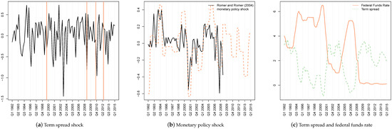
Figure 1.
Term spread and monetary policy shock. Notes: The plot in the left panel shows the identified term spread shock. Vertical bars refer to the launch of the Clinton debt buyback program and the three LSAP programs. The middle panel shows the monetary policy shock along with the narrative monetary policy shock of Romer and Romer (2004). The right panel shows the evolution of the term spread and the federal funds rate (realized data).
Looking at the term spread shock first, we have indicated three distinct time periods by red vertical bars, namely the start of the Clinton debt buyback program (Q1 2000–Q4 2001), which was in many ways similar to an LSAP, and the start of LSAPs I–III (Q4 2008, Q4 2010 and Q3 2012; see (Dunne et al. 2015)). The figure shows that negative surprises to the term spread indeed coincide with these periods. There is also a pronounced negative shock visible in the last quarter of 2003 in which the term spread started to decrease sharply (see the right panel, Figure 1).
The monetary policy shock is shown in the middle panel. For comparison, we also plot a monetary policy shock series based on the narrative approach put forward in Romer and Romer (2004), extended to cover the period up until Q4 2008.11 Both shocks identified the same monetary policy cycle, and the correlation between the series amounted to about 0.6.
3.1. How Do Term Spread and Monetary Policy Shocks Affect Output Growth and Inflation?
In this section, we examine through which channels both shocks affect aggregate demand and CPI inflation. To this end, we report impulse response functions in Figure 2 and Figure 3 and a related forecast error variance decomposition in Table 2. Since we use a time-varying framework, the reported impulse responses showed how the economy would react to a hypothetical shock at a specific point in time. This holds equally true for sample periods where actually no monetary policy/spread shock occurred.12 Both shocks were normalized to a 100 basis point (bp) reduction, either of the policy rate (monetary policy shock) or the term spread (spread shock). Results are shown for real GDP growth, inflation, wealth growth and banking sector variables.
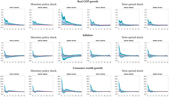
Figure 2.
Impulse response functions. Notes: Posterior median responses to an expansionary monetary policy shock (−100 bp) and shock to the term spread (−100 bp) along with 50% (dark blue) and 68% (light blue) credible bounds. Results shown as averages over three periods, pre-crisis from 1991Q1–2007Q3, global financial crisis from 2007Q4–2009Q2 and its aftermath from 2009Q3–2015Q1.
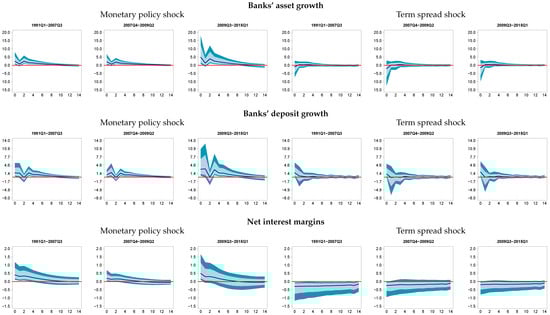
Figure 3.
Impulse response functions. Notes: Posterior median responses to an expansionary monetary policy shock (−100 bp) and shock to the term spread (−100 bp) along with 50% (dark blue) and 68% (light blue) credible bounds. Results shown as averages over three periods, pre-crisis from 1991Q1–2007Q3, global financial crisis from 2007Q4–2009Q2 and its aftermath from 2009Q3–2015Q1.
Table 2.
Forecast error variance decomposition.
The top panel of Figure 2 lists results for real output growth: on the left-hand side in response to the conventional monetary policy shock and on the right-hand side in reaction to the term spread shock. Note that we have opted for slicing the time-varying impulse responses by fixing time periods of interest to show accompanying credible sets (50% in dark blue and 68% in light blue). These periods relate to the global financial crisis, namely the pre-crisis period (Q1 1991–Q3 2007), the crisis period (Q4 2007–Q2 2009) and its aftermath (Q3 2009–Q1 2015).13
Looking at the unexpected lowering of the policy rate first, we find positive and tightly estimated responses up until eight quarters, indicating rather persistent effects on output growth. This holds true throughout the sample periods considered. The size of the effects, however, varies with the period under consideration. More specifically, the 100-bp decrease in the policy rate accelerates real GDP growth on impact by around 0.3–0.4 percentage points prior to and during the crisis. In the aftermath of the global financial crisis, this effect increases markedly to about 0.7 percentage points.14 To put our results into perspective, we compare the cumulative responses with established findings of the literature, which are mainly based on pre-crisis data. In cumulative terms, the responses prior to the crisis point to an increase in real GDP by 1.8%, whereas previous findings indicate peak level effects of about 0.3%–0.6%; see, e.g., (Bernanke et al. 1997; Leeper et al. 1996; Uhlig 2005). In a more recent paper, Gorodnichenko (2005) reported a peak effect in real GDP of approximately 0.8%. See Coibion (2012) for an excellent and more comprehensive summary of the relevant literature.
Responses of output growth to the lowering of the term spread are depicted on the right-hand side of the top panel of Figure 2. The term spread shock accelerates real GDP growth throughout the sample period. Our estimates are broadly in line with those provided in Baumeister and Benati (2013), who report an annualized impact response of about 2% for 2010. Compared to findings on the conventional monetary policy shock, however, the effects of the term spread shock are rather short-lived and peter out after one to two quarters. This finding is in contrast to Inoue and Rossi (2018), who proposed identifying conventional and unconventional monetary policy shocks in a unified manner by modeling an exogenous shift of the whole term structure. Their results imply similar effects of conventional on unconventional monetary policy on both output growth and inflation. In Table 2, we present a forecast error variance decomposition. At the 20-quarter forecast horizon, the monetary policy shock explains about 20%–30% more forecast error variance than the spread shock.
The middle panel of Figure 2 shows impulse responses of consumer price inflation. Both shocks drive up inflation by about 0.2–0.3 percentage points on impact, as we have ruled out a price puzzle by assumption. Adjustment of inflation turns negative in response to lowering the policy rate, while effects are positive and then quickly converge to zero in response to the spread shock. The spread shock accounts for a larger part of forecast error variance throughout the sample period. Summing up, we find that both shocks accelerate output growth and drive up inflation. While the effects of a conventional monetary policy shock on output growth are rather persistent and tightly estimated, the effects of the term spread shock are short-lived. Responses of CPI inflation are accompanied by wide credible sets for both shocks.
3.2. The Transmission of Monetary Policy and Term Spread Shocks
In this section, we analyze the potential transmission mechanisms starting with the wealth channel. In the bottom panel of Figure 2, we depict responses for consumer wealth growth. Looking at the conventional monetary policy shock first, we find positive responses of consumer wealth throughout most of the sample period. These effects, however, are very short-lived and peter out immediately after impact. By contrast, the reduction of the term spread spurs wealth growth throughout the sample periods, and effects tend to be slightly more persistent compared to responses to the monetary policy shock discussed before. In terms of forecast error variance and with the exception of the period of the global financial crisis, the term spread shock explains about 1.5–2-times as much variance as the monetary policy shock. Taken at face value, the results reveal the wealth channel as an important facet of the transmission mechanism through which unconventional monetary policy can affect aggregate demand. In terms of persistence, the channel seems less important when monetary policy is conducted by steering short-term interest rates. This result is in line with Ludvigson et al. (2002), who attest the wealth channel having only a minor role in the transmission of conventional monetary policy to consumption.
Next, we investigate the bank lending/credit channel. Figure 3 shows the responses of growth in assets and deposits of commercial banks, as well as net interest rate margins and Table 2 the corresponding forecast error variance decomposition.
The impact response of asset growth to a conventional monetary policy shock is shown in the top panel of the figure. A loosening of monetary policy spurs asset growth for all three time periods considered; responses are tightly estimated; and the effects tend to be very persistent. Next, we look at the growth of deposits depicted in the middle panel of Figure 3. Albeit that for both shocks, we have assumed an immediate acceleration of deposit growth, the effects of the term spread immediately peter out after one quarter, while responses to the conventional monetary policy shock are rather persistent and mostly tightly estimated. That is, the impact of the term spread shock on asset and deposit growth is negligible, while we find tightly estimated responses to the conventional monetary policy shock. This impression is broadly confirmed by a forecast error variance decomposition, shown in Table 2. At the 20-quarter forecast horizon, the spread shock accounts for 11% of both the error variance of banks’ asset and deposit growth. Shares of explained variance in banks’ deposit growth are comparable to that explained by the spread shock. Shares related to banks’ asset growth explained by the monetary policy shock are somewhat higher. Strong and persistent effects of a conventional monetary policy shock on asset and deposit growth and a large share of explained forecast error variance reveal an important role for the credit/bank lending channel for monetary policy transmission. By contrast, this channel seems less important in the case that the stimulus comes from lowering the term spread.
For completeness, we show responses of net-interest rate margins in the bottom panel of Figure 3. An unexpected decrease of the policy rate triggers an increase in net interest rate margins, probably driven by an imperfect pass through of the policy rate change to the long end of the yield curve. After four quarters, effects start hovering around zero and are accompanied by wide credible sets. Responses to the term spread shock show a different pattern: net interest rate margins decrease in response to a lowering of the term spread. These effects are very persistent for all three time periods considered. Naturally, and since net interest margins follow the term spread, the term spread shock explains considerably more forecast error variance as the conventional monetary policy shock. This holds true throughout the sample period.
Summing up, positive effects on output growth seem to be driven by an expansion of asset and deposit growth of the banking sector, lending empirical support for the importance of the credit/bank lending channel in case stimulus comes from lowering the policy rate. By contrast, the spread shock has no significant effect on asset and deposit growth. Rather, positive (and short-lived) effects on output growth are triggered by an acceleration of consumer wealth growth.
3.3. Do Effects Vary over Time?
Having established through which channels both shocks transmit to the real economy, we now investigate more closely their overall effects. The strength of both shocks might depend on the specific economic environment when the shock is carried out. For example, Jannsen et al. (2014) found strong effects of monetary policy during recessions associated with financial crises, which holds especially true for the recent global financial crisis. They attribute their finding to the particular effectiveness of the credit/bank lending channel in a recession, as advocated in Bernanke and Gertler (1995). Others find the opposite, namely that monetary policy is less effective in times of heightened uncertainty (Aastveit et al. 2017; Bech et al. 2014). Considering the term spread shock, recent empirical research hints at diminishing effectiveness of the LSAP programs; see, e.g., (Wu 2014).
So far, results reported in Figure 2 and Figure 3 have indicated changes in the strength of the shocks’ impacts on the variables considered in this study. However, these results might be driven by the normalization of the shocks to 100 basis points, which is achieved by dividing through the impact response of the short-term interest rate and the term spread (both which have diminished strongly, since the period the FFR is technically zero). To investigate this further, we report the ratio of the cumulative response after 20 quarters to the one standard deviation shock on impact, with the standard deviation varying over the sample. These “elasticities” are thus free of the normalization effect and show the responsiveness of a given variable in cumulative terms to the two shocks on impact over the sample period.
Elasticities shown in Figure 4 reveal a very systematic pattern over time. Stimulus from conventional monetary policy is less effective during the period of the global financial crisis compared to prior to the crisis. This is particularly so in terms of output growth for which the elasticity reaches its trough over the whole sample period during the crisis. Hence, we qualitatively corroborate the findings of Bech et al. (2014), Aastveit et al. (2017), Hubrich and Tetlow (2015), who attributed smaller effects of monetary policy during financial crises to balance sheet adjustments and the deleveraging of the private sector. on the one hand, and heightened uncertainty weighing on the business climate, on the other hand. Strikingly, elasticities in the aftermath of the crisis do not simply revert back to their pre-crisis values. The responsiveness of all variables except net interest rate margins evens peaks during the aftermath of the crisis. This finding is certainly less related to the episode of the crisis and its long-lasting consequences for the economy. Rather, the specific monetary environment with the policy rate bound at zero seem to drive this result. Taken at face value, our finding implies that monetary policy is particularly effective if the policy rate is altered after it has been committed to a particular value for a prolonged time.
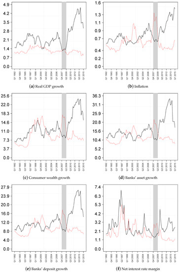
Figure 4.
Elasticity of cumulative response to the size of shock on impact. Notes: The figure shows the ratio of the cumulative response of particular variable to the impact shock of the conventional monetary policy shock (black, solid line) and the spread shock (red, dashed line). Elasticities are in absolute terms. The shaded grey area indicates the period of the recession associated with the global financial crisis.
Elasticities related to the term spread shock spike for most variables during the crisis and during the period from 2000–2001. In the latter period, the Clinton debt buyback program took place, which was in many ways similar to an LSAP. See Greenwood and Vayanos (2010) for an in-depth analysis of the buyback program and its effect on the Treasury yield curve. This time pattern holds in particular true for inflation, consumer wealth and growth in bank’s assets and deposits. The effects of lowering the term spread on output growth have also diminished after the launch of the first LSAP. Our findings thus ascribe the latter to LSAPs’ smaller effects on the macroeconomy than the first programs, corroborating the results of Wu (2014) and Engen et al. (2015). The work in Engen et al. (2015) explicitly attributed the stronger effects of the earlier programs to the fact that they have been implemented at times when market conditions were highly strained, and a signal of commitment to accommodative policy over a longer horizon—such as the launch of quantitative easing—would be most effective.
Summing up, we find that monetary policy effectiveness in boosting aggregate demand decreases significantly in the run-up of the global financial crisis. In the aftermath of the crisis, however, a hypothetical monetary policy shock would lead to strong effects on output growth and inflation. The opposite holds true for the spread shock, which is particularly stimulating during the period of the crisis when the Fed’s engagement in quantitative easing served as an important signal to longer term accommodative monetary policy. In the aftermath of the crisis, the effectiveness of the hypothetical spread shock declines.
3.4. Did Term Spread and Monetary Policy Shocks Matter Historically?
Last, we examine the contribution of both shocks in explaining deviations from trend growth in the variables under consideration. These are depicted in Figure 5. We would expect higher contributions of the monetary policy shock prior to the global financial crisis and increasing contributions of the spread shock thereafter. The historical decomposition of most time series actually corroborates this presumption. More specifically, monetary policy shocks explain larger shares of movements in real GDP growth, inflation and banks’ asset growth prior to and after the global financial crisis. However, the ratio of monetary policy to spread shock contribution declined significantly from end-2008 to the end of our sample. Even more visible are contributions related to the term spread, banks’ deposit growth, consumer wealth growth and net interest margins, for which the spread shock explains a considerably larger part of movements than the monetary policy shock in the aftermath of the crisis.
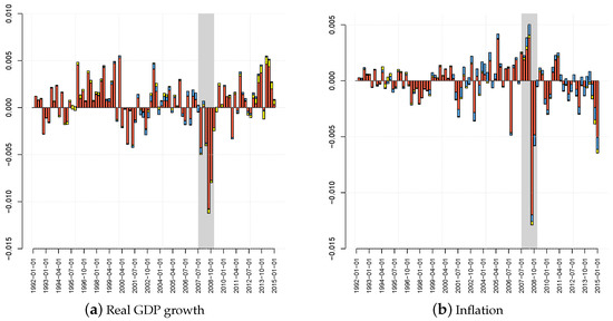
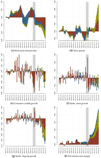
Figure 5.
Historical decomposition of time series. Notes: Historical decomposition of time series based on the posterior median. The overall contribution of all shocks except the term spread and monetary policy shock in red. Contributions of the monetary policy shock and the term spread shock in blue and yellow, respectively. The shaded grey area indicates the period of the recession associated with the global financial crisis.
Summing up, a historical decomposition analysis revealed that the monetary policy shock can explain movements in real GDP growth and inflation to a comparably larger extent than the spread shock throughout the sample period. By contrast, the spread shock explains movements in the term spread, consumer wealth growth, banks’ deposit growth and net interest margins to a comparably larger extent. For all variables considered, the importance of the spread shock has increased significantly since end-2008, the period in which the first LSAP was launched. This finding is in line with our expectations and thus leads to further confidence in the statistical framework used in this study.
3.5. Robustness and Extensions
In this section, we investigate the robustness of our results. We do this by first looking at another measure of banks’ asset growth taking a broader definition of the banking sector, by including investment growth as a further variable to the system and last by imposing different orderings of the variables to demonstrate that our estimates remain qualitatively unaffected.
First, since the shadow banking sector has expanded rapidly over the last decade in the USA, it has been argued that focusing on commercial banks’ assets might yield an incomplete assessment of monetary policy transmission; see, e.g., (Adrian et al. 2010; Nelson et al. 2018). Hence, we substitute commercial banks’ assets with assets of the shadow banking sector and re-run the analysis outlined in Section 3. Shadow banks are defined as financial intermediaries that conduct functions of banking without access to central bank liquidity and, in the definition following Nelson et al. (2018), comprise finance companies, issuers of asset-backed securities and funding corporations.15 In a nutshell, credit intermediation through the shadow banking system is comparable to credit intermediation of a traditional bank with wholesale investors at the deposit end, and at the loan origination end are finance companies and traditional banks.
Figure 6 shows impulse responses of asset growth, deposit growth and real GDP growth. Overall, results on real activity are nearly unaffected by inclusion of shadow assets, albeit the uncertainty of the estimates is slightly more elevated especially in the most recent part of our sample. While the shape of asset and deposit growth responses is very similar to our baseline estimates, including shadow assets yields stronger responses in terms of overall magnitudes. This holds true for all time periods considered, for both shocks and for both variables. However, these stronger magnitudes are estimated with much uncertainty and hence do not translate into overall stronger responses of real GDP growth. The responses of the other variables are very similar to the results of our baseline estimation. This is also evident from Table 3, top panel, which lists correlations of median impulse responses with the baseline model. The fact that we get very similar results of asset responses to both shocks contrasts the findings of Nelson et al. (2018), who reported a decrease of commercial banks’ assets and an increase of shadow assets in response to a contractionary monetary policy shock. Note that we have not restricted the responses of asset growth, and our results are hence purely data driven. They might differ from those of Nelson et al. (2018) since we use a richer framework in terms of included variables and covered transmission channels.
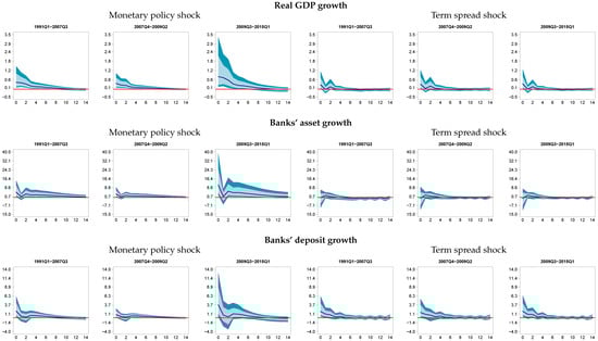
Figure 6.
Impulse responses with shadow assets. Notes: Posterior median responses to an expansionary monetary policy shock (−100 bp) and shock to the term spread (−100 bp) along with 50% (dark blue) and 68% (light blue) credible bounds. Results shown as averages over three periods, pre-crisis from 1991Q1–2007Q3, global financial crisis from 2007Q4–2009Q2 and its aftermath from 2009Q3–2015Q1. Results based on inclusion of assets of the shadow banking sector instead of commercial banks’ assets.
Table 3.
Correlation of median impulse responses.
Second, and as pointed out in Stein (2012), a reason why the effects of asset purchase programs might have diminished over time are smaller effects via investment spending. In principle, a decrease in longer term borrowing costs for firms should boost investment spending. If, however, borrowing costs are further reduced by additional asset purchase programs, firms might simply pay back short-term debt and issue more and less expensive long-term debt. In that case, there is no additional impetus to the economy via investment spending. To investigate this in more depth, we re-run our analysis with gross fixed investment growth as an additional variable. We also modify the characterization of the two shocks provided by the restrictions in Table 1. Here, we add further restrictions saying that investment growth ticks up in response to both, a conventional monetary policy expansion and a shock to the term spread. Figure 7 shows the elasticity of the cumulative response with respect to the initial size of the shock.
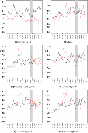
Figure 7.
Elasticity of cumulative response to size of shock on impact; investment growth included. Notes: The figure shows the ratio of the cumulative response of a particular variable to the impact shock of the conventional monetary policy shock (black, solid line) and the spread shock (red, dashed line). Elasticities are in absolute terms. The shaded grey area indicates the period of the recession associated with the global financial crisis.
Looking at investment growth points indeed to a smaller elasticity in the aftermath of the crisis compared to the crisis period itself. The pattern of the other variables is consistent with our baseline estimates, stronger effects during the crisis and smaller impacts in the aftermath regarding the term spread shock, while the opposite holds true for the monetary policy shock. In general, including investment growth has rendered elasticities more volatile in the aftermath of the crisis. This is due to the fact that with the additional restrictions imposed, it is harder to find rotation matrices fulfilling the complete set of identifying assumptions. More specifically, while impulse responses of our baseline estimate are typically based on 250–300 rotation matrices each ten quarters we sample them, the number of successfully sampled matrices decreases to about 150 per sampling point when including investment growth. Considering impulse responses (available from the authors upon request), the inclusion of investment growth leaves our results broadly unchanged.
Last and to add further confidence to our results, we change the ordering of the variables for our estimation setup. For the baseline ordering, we put real GDP growth first, followed by inflation, wealth, short-term interest rates, banks’ deposits and assets, the term spread and net interest rate margins. This ordering is motivated in Christiano et al. (1996) and states that output cannot be contemporaneously affected by inflation, consumer wealth and the policy rate. Results of the baseline ordering are compared to results under 10 randomly chosen orderings. As stressed before and since we rely on an explicit identification of the shocks via sign restrictions, the ordering of the variables should not affect our results qualitatively. This is evident in the bottom panel of Table 3, which shows average correlations of median impulse responses under the baseline and the 10 permuted orderings. In fact, correlations are in almost all cases virtually unity. These small differences can be well attributed to sampling error.
4. Conclusions
In this paper, we have analyzed the effects and transmission of conventional and unconventional monetary policy in the USA. For that purpose, we have proposed a medium- to large-scale model that allows parameters to drift and residual variances to change over time. Our main results remain qualitatively unaffected when considering an alternative measure for banking sector assets, including investment growth as a further transmission channel and using different Cholesky orderings in the estimation stage of the model. These can be summarized as follows:
First, we discuss the monetary policy shock. The rate cut has positive and rather persistent effects on output growth. These are driven by an expansion of asset and deposit growth of the banking sector and thus by a broad credit/bank lending channel. By contrast and in line with previous findings (see, e.g., (Ludvigson et al. 2002)), the wealth channel appears less important for the transmission of conventional monetary policy in the USA. A forecast error variance decomposition lends further support to these findings. More importantly though, we find a pronounced and distinct pattern of monetary policy effectiveness over time. More specifically, our results point to comparably modest effects on output growth in response to a hypothetical and unexpected lowering of the policy rate during the period of the global financial crisis. In this sense, our results corroborate the findings of a recent strand of the literature stating that monetary policy is weak in recessions associated with either high economic uncertainty or more generally financial crises; see, e.g., (Aastveit et al. 2017; Bech et al. 2014; Hubrich and Tetlow 2015; Tenreyro and Thwaites 2016). There is less empirical work on the effectiveness of monetary policy in the aftermath of the global financial crisis, a period in which the main U.S. policy rate was effectively zero. Our results show the strongest responsiveness of the economy to a hypothetical monetary policy shock during that period. From the perspective of a policymaker, this seems less relevant in practical terms, since obviously, the policy rate cannot enter negative territory. However, it is rather the fact that the policy rate has not changed for an extended time than the level at which the policy rate stood that drives this result. If changes in the policy rate are rare, volatility associated with a monetary policy shock is low, and a deviation from the commitment can provide a particularly strong boost to output growth. Note, however, that a central bank’s loss function typically consists of other additional targets such as price stabilization, and hence, our finding does not directly translate into a policy recommendation to deviate from a commitment. Still, it suggests that effects of a correction of the monetary policy stance after an extended period of unchanged monetary policy might have large macroeconomic effects.
Second, and looking at the term spread shock, we find positive, but short-lived effects on output and consumer price growth. These work mainly through the consumer wealth channel and via steering inflation, while there is less evidence of impetus via banks’ asset and deposit growth. Effects of the term spread shock show also a distinct pattern over time. More specifically, we find that the term spread shock impacts most strongly the output growth during the period of the global financial crisis and less so in its aftermath. Taken at face value, this result implies that the effectiveness of the Fed’s unconventional monetary policy measures has abated since the early programs. Smaller effects in the most recent period stem from a decrease in stimulus of consumer wealth and a smaller responsiveness of inflation. These might be attributed to an implicit signaling channel, which is particularly effective when financial markets are impaired and economic conditions are characterized by high uncertainty (Engen et al. 2015). In addition, we show that effects of quantitative easing on investment growth have diminished over time providing, thereby less stimulus for overall GDP growth.
Author Contributions
Conceptualization, M.F. and F.H.; methodology, F.H.; software, F.H.; validation, M.F., F.H.; formal analysis, M.F. and F.H.; investigation, M.F.; resources, M.F.; data curation, M.F.; writing—original draft preparation, M.F.; writing—review and editing, F.H.; visualization, M.F.; supervision, M.F. and F.H.; project administration, M.F.
Funding
This research received no external funding.
Conflicts of Interest
The authors declare no conflict of interest.
Appendix A. Structural Identification
To implement the sign restrictions technically, note that Equation (8) can be written as:
where and is a standard normal vector error term. Multiplication from the left by yields:
with and .
It can be shown that left multiplying Equation (A2) with an -dimensional orthonormal matrix with leaves the likelihood function untouched. This implies that impulse responses are set-identified. To implement the sign restrictions approach, we simply draw using the algorithm outlined in Rubio-Ramírez et al. (2010) until the impulse response functions satisfy a given set of sign restrictions to be chosen by the researcher. This has to be done for each draw from the posterior, which in our application boils down to 500 draws randomly taken from the full set of 15,000 posterior draws. To speed up computation, we do not search for each point in time a new rotation matrix. Instead, we look for new rotation matrices after 10 quarters and check whether the restrictions are fulfilled throughout the sample. These leaves us with 11 time periods for which we look for new rotation matrices. For each of these time points, we recovered 250–300 rotation matrices that fulfilled our restrictions. There was no visible time pattern over the amount of sign restrictions recovered throughout our sample period.
To impose the additional restriction that the short-term interest rate reacts sluggishly with respect to an unconventional monetary policy shock, we construct the following deterministic rotation matrix (Baumeister and Benati 2013):
with:
The rotation angle is defined as:
Here, the notation selects the -th element of the impact matrix, corresponding to the contemporaneous response of variable the short-term interest rate (variable i) to an unconventional monetary policy shock (variable j). Multiplying the impact matrix with from the right yields a new impact matrix that satisfies the set of sign restrictions specified in Section 2.4 and the zero impact restriction described above.
Since we assume that the central bank is constrained by the zero lower bound, we zero-out the structural coefficients of the monetary policy rule for the first eight quarters after the shock hit the economy. This procedure, however, is subject to the Lucas critique because economic agents are not allowed to change their behavior accordingly. However, the findings in Baumeister and Benati (2013) suggest that the differences between the results obtained by manipulating the structural coefficients or by manipulating the historical structural shocks to keep the interest rate at the zero lower bound are quite similar. Moreover, manipulating the structural shocks gives rise to additional shortcomings like the fact that this approach ignores the impact of agents expectations about future changes in the policy rate. In addition, the systematic component of monetary policy implies that the short-term interest rate reacts to different shocks. However, the unsystematic part, by construction, offsets this behavior, and the corresponding shocks would no longer originate from a white noise process.
Appendix B. A Brief Sketch of the Markov Chain Monte Carlo Algorithm
Since we impose a Cholesky structure on the model a priori and estimate the system equation-by-equation, our Markov chain Monte Carlo (MCMC) algorithm consists of the following three steps:
- Sample and using the algorithm of Carter and Kohn (1994).
- Sample and the corresponding parameters of Equation (7) through the algorithm put forth in Kastner and Frühwirth-Schnatter (2013). A brief description of this algorithm is provided in Appendix C.
Step 1 is a standard application of Gibbs sampling in state-space models. In Step 2, we draw the parameters of the corresponding state equations conditional on the states. Step 3 is described in more detail in the Appendix. Finally, note that we sample the parameters of the different equations simultaneously.
Appendix C. Sampling Log-Volatilities
To simulate the full history of log-volatilities for the i-th equation , we use the algorithm outlined in Kastner and Frühwirth-Schnatter (2013). This algorithm samples , all without a loop. This is achieved by rewriting in terms of a multivariate normal distribution. Moreover, the parameters of the state equation in Equation (7) are sampled through simple Metropolis–Hastings (MH) or Gibbs sampling steps. To achieve a higher degree of sampling efficiency, we sample the corresponding parameters from the centered parameterization in Equation (7) and a non-centered variant given by:
To simplify the exposition, we illustrate the algorithm for the case when . For , the same steps apply with only minor modifications. Let us begin by rewriting Equation (4) as:
Squaring and taking logarithms yield:
Since follows a distribution, we use a mixture of Gaussian distribution to render Equation (A8) conditionally Gaussian,
where is an indicator controlling the mixture component to use at time twith . and define the mean and the variance of the mixture components employed.
The mixture indicators allow us to rewrite Equation (A8) as a linear Gaussian state space model:
The algorithm then consists of the following steps.
- Sample or , all without a loop (AWOL). Here, is a vector of stacked coefficients and . Following Rue (2001), can be written in terms of a multivariate normal distribution:Similarly, the normal distribution corresponding to the non-centered parameterization is given by:The corresponding posterior moments are:and:Multiplying by yields the moments for the non-centered parameterization: and . Finally, the initial states of , and are obtained from their respective stationary distributions.
- Obtain the parameters of Equation (7) and Equation (A8). Since we impose a non-conjugate Gamma prior on , we employ a Metropolis-within-Gibbs algorithm to sample and for both parameterizations. For the centered variant, we simulate and with a single Gibbs step, and is sampled through an MH step. For the non-centered parameterization, we sample with MH and the other parameters with Gibbs steps.
- Sample the mixture indicators with inverse transform sampling. Note that we can rewrite Equation (A8) as:This allows us to compute the posterior probabilities that , which are given by:where are the unnormalized weights associated with the c-th mixture component.
The algorithm simply draws the parameters under both parametrizations and decides ex-post which of the parametrizations to use. This choice depends on the relationship between the variances of Equations (7) and (A8). For more information, see Kastner and Frühwirth-Schnatter (2013) and Kastner (2013).
The sampled log-volatilities are shown in Figure A1.

Figure A1.
Stochastic volatility over time. Notes: Posterior mean of residual variance over time.
Reduced form volatility of the short-term interest rate and the term spread has increased considerably in the run-up of the global financial crisis, a period during which the Fed has aggressively lowered interest rates. Volatility has spiked around mid-2008 and hence in the midst of the crisis. While the crisis peak of residual variance associated with the short-term interest rate marked also the peak over our sample period, volatility of the term spread peaked in the early 1990s.
The middle panel of Figure A1 shows the volatilities for variables related to the real side of the economy. Residual variance associated with real GDP growth was elevated in the early 2000s and peaked around the same time as the financial variables discussed above. During the early 2000s, the so-called “dot-com bubble” burst, causing the slowing down of the U.S. economy. Stochastic volatility of wealth, which is strongly anchored on movements in stock market prices, naturally was also elevated during that period. In contrast to the volatility of real GDP, residual variance of wealth was pronounced for a longer period during the global financial crisis. Residual variance of CPI inflation started to rise more considerably from the beginning of the 2000s until 2008, a period that was characterized by sound growth in price dynamics in the USA. Residual variance peaked in the aftermath of the crisis and hence a little later than that associated with real GDP growth, when CPI inflation reverted from negative to positive territory.
Last, the bottom panel of Figure A1 shows residual variance for variables related to the banking sector. Residual variance of asset growth of commercial banks was elevated during the early 2000s and the global financial crisis, where it peaked around the same time as residual variance of real GDP growth, short-term interest rates and the term spread. Since 2009, estimated volatility has declined and is considerably smaller in the most recent period in our sample compared to its peak value. Residual variance associated with bank deposits and net interest margins show a slightly different pattern. Bank deposit volatility increased gradually from the beginning of 2004 until 2009, after which it gradually started to decline until the end of our sample period. Volatility associated with net interest margins spiked around 1997 and peaked in late 2009. That is, for both variables, banking deposits and net interest margins, volatility spikes during the global financial crisis occurred slightly later than those of the other variables considered in this study.
References
- Aastveit, Knut Are, Gisle James Natvik, and Sergio Sola. 2017. Economic uncertainty and the influence of monetary policy. Journal of International Money and Finance 76: 50–67. [Google Scholar] [CrossRef]
- Adrian, Tobias, Emanuel Moench, and Hyun Song Shin. 2010. Financial Intermediation, Asset Prices, and Macroeconomic Dynamics. Staff Reports 422. New York: Federal Reserve Bank of New York. [Google Scholar]
- Adrian, Tobias, and Hyun Song Shin. 2010. Financial Intermediaries and Monetary Economics. In Handbook of Monetary Economics. Edited by Benjamin. M. Friedman and Michael Woodford. Amsterdam: Elsevier, vol. 3, chp. 12. pp. 601–50. [Google Scholar]
- Baumeister, Christiane, and Luca Benati. 2013. Unconventional Monetary Policy and the Great Recession: Estimating the Macroeconomic Effects of a Spread Compression at the Zero Lower Bound. International Journal of Central Banking 9: 165–212. [Google Scholar]
- Baumeister, Christiane, and James D. Hamilton. 2015. Sign restrictions, structural vector autoregressions, and useful prior information. Econometrica 83: 1963–99. [Google Scholar] [CrossRef]
- Bech, Morten L., Leonardo Gambacorta, and Enisse Kharroubi. 2014. Monetary Policy in a Downturn: Are Financial Crises Special? International Finance 17: 99–119. [Google Scholar] [CrossRef]
- Benati, Luca, and Charles Goodhart. 2008. Investigating time-variation in the marginal predictive power of the yield spread. Journal of Economic Dynamics and Control 32: 1236–72. [Google Scholar] [CrossRef]
- Bernanke, Ben S., and Alan S. Blinder. 1988. Credit, Money, and Aggregate Demand. American Economic Review 78: 435–9. [Google Scholar]
- Bernanke, Ben S., and Mark Gertler. 1995. Inside the Black Box: The Credit Channel of Monetary Policy Transmission. Journal of Economic Perspectives 9: 27–48. [Google Scholar] [CrossRef]
- Bernanke, Ben S., Mark Gertler, and Mark Watson. 1997. Systematic Monetary Policy and the Effects of Oil Price Shocks. Brookings Papers on Economic Activity 28: 91–157. [Google Scholar] [CrossRef]
- Black, Lamont, Diana Hancock, and Waynee Passmore. 2007. Bank Core Deposits and the Mitigation of Monetary Policy; Technical Report 65; Federal Reserve Board Finance and Economics Discussion Series; Washington: Federal Reserve Board.
- Bloom, Nicholas. 2009. The Impact of Uncertainty Shocks. Econometrica 77: 623–85. [Google Scholar]
- Boivin, Jean, and Marc P. Giannoni. 2006. Has Monetary Policy Become More Effective? The Review of Economics and Statistics 88: 445–62. [Google Scholar] [CrossRef]
- Boivin, Jean, Michael T. Kiley, and Frederic S. Mishkin. 2010. How Has the Monetary Transmission Mechanism Evolved Over Time? In Handbook of Monetary Economics. Edited by Benjamin. M. Friedman and Michael Woodford. Amsterdam: Elsevier, vol. 3, chp. 8. pp. 369–422. [Google Scholar]
- Breitfuß, Sebastian, Martin Feldkircher, and Florian Huber. 2018. Changes in U.S. monetary policy and its transmission over the last century. German Economic Review. [Google Scholar] [CrossRef]
- Butt, Nick, Rohan Churm, Michael McMahon, Arpad Morotz, and Jochen Schanz. 2014. QE and the Bank Lending Channel in the United Kingdom. Working Paper 511. London: Bank of England. [Google Scholar]
- Carriero, Andrea, Todd E Clark, and Massimiliano Marcellino. 2015. Large Vector Autoregressions With Asymmetric Priors. Working Paper Series (2015/759); London: Queen Mary University of London. [Google Scholar]
- Carter, Chris K., and Robert Kohn. 1994. On gibbs sampling for state space models. Biometrika 81: 541–53. [Google Scholar] [CrossRef]
- Christiano, Lawrence J., Martin Eichenbaum, and Charles Evans. 1996. The Effects of Monetary Policy Shocks: Evidence from the Flow of Funds. The Review of Economics and Statistics 78: 16–34. [Google Scholar] [CrossRef]
- Christiano, Lawrence J., Martin Eichenbaum, and Charles L. Evans. 2005. Nominal rigidities and the dynamic effects of a shock to monetary policy. Journal of Political Economy 113: 1–45. [Google Scholar] [CrossRef]
- Cogley, Timothy, Sergei Morozov, and Thomas J. Sargent. 2005. Bayesian fan charts for uk inflation: Forecasting and sources of uncertainty in an evolving monetary system. Journal of Economic Dynamics and Control 29: 1893–925. [Google Scholar] [CrossRef]
- Cogley, Timothy, and Thomas J. Sargent. 2002. Evolving Post-World War II U.S. Inflation Dynamics. In NBER Macroeconomics Annual 2001. Cambridge: National Bureau of Economic Research, Inc., vol. 16, NBER Chapters. pp. 331–88. [Google Scholar]
- Cogley, Timothy, and Thomas J. Sargent. 2005. Drifts and volatilities: Monetary policies and outcomes in the post wwii us. Review of Economic Dynamics 8: 262–302. [Google Scholar] [CrossRef]
- Coibion, Olivier. 2012. Are the Effects of Monetary Policy Shocks Big or Small? American Economic Journal: Macroeconomics 4: 1–32. [Google Scholar] [CrossRef]
- Doh, Taeyoung. 2010. The efficacy of large-scale asset purchases at the zero lower bound. Economic Review 95: 5–34. [Google Scholar]
- Dunne, Peter, Mary Everett, and Rebecca Stuart. 2015. The Expanded Asset Purchase Programme—What, Why and How of Euro Area QE. Quarterly Bulletin Articles. Dublin: Central Bank of Ireland, pp. 61–71. [Google Scholar]
- Engen, Eric M., Thomas T. Laubach, and David Reifschneider. 2015. The Macroeconomic Effects of the Federal Reserve’s Unconventional Monetary Policies; Finance and Economic Discussion Series 2015-005; Washington: Board of Governors of the Federal Reserve System (U.S.).
- Fawley, Brett W., and Luciana Juvenal. 2012. Quantitative easing: Lessons we’ve learned. The Regional Economist 7: 8–9. [Google Scholar]
- Fernández-Villaverde, Jesús, Pablo Guerró-Quintana, Juan F. Rubio-Ramírez, and Martin Uribe. 2011. Risk matters: The real effects of volatility shocks. American Economic Review 101: 2530–61. [Google Scholar] [CrossRef]
- Frühwirth-Schnatter, Sylvia. 1994. Data augmentation and dynamic linear models. Journal of Time Series Analysis 15: 183–202. [Google Scholar] [CrossRef]
- Fry, Renée, and Adrian Pagan. 2011. Sign restrictions in structural vector autoregressions: A critical review. Journal of Economic Literature 49: 938–60. [Google Scholar] [CrossRef]
- Gagnon, Joseph, Matthew Raskin, Julie Remache, and Brian Sack. 2011. The Financial Market Effects of the Federal Reserve’s Large-Scale Asset Purchases. International Journal of Central Banking 7: 3–43. [Google Scholar]
- Gertler, Mark, and Peter Karadi. 2015. Monetary policy surprises, credit costs, and economic activity. American Economic Journal: Macroeconomics 7: 44–76. [Google Scholar] [CrossRef]
- Gorodnichenko, Yuriy. 2005. Reduced-Rank Identification of Structural Shocks in VARs. Macroeconomics 0512011. Germany: University Library of Munich. [Google Scholar]
- Greenwood, Robin, and Dimitri Vayanos. 2010. Price Pressure in the Government Bond Market. American Economic Review 100: 585–90. [Google Scholar] [CrossRef]
- Hamilton, James D. 2018. The Efficacy of Large-Scale Asset Purchases When the Short-term Interest Rate is at its Effective Lower Bound. Brookings Papers on Economic Activity. Washington: Brookings Press. [Google Scholar]
- Hamilton, James D., and Jing Cynthia Wu. 2012. The Effectiveness of Alternative Monetary Policy Tools in a Zero Lower Bound Environment. Journal of Money, Credit and Banking 44: 3–46. [Google Scholar] [CrossRef]
- Hubrich, Kirstin, and Robert J. Tetlow. 2015. Financial stress and economic dynamics: The transmission of crises. Journal of Monetary Economics 70: 100–15. [Google Scholar] [CrossRef]
- Inoue, Atsushi, and Barbara Rossi. 2018. The Effects of Conventional and Unconventional Monetary Policy on Exchange Rates. NBER Working Papers 25021. Cambridge: National Bureau of Economic Research, Inc. [Google Scholar]
- Ireland, Peter N. 2005. The Monetary Transmission Mechanism. Working Papers 06-1. Boston: Federal Reserve Bank of Boston. [Google Scholar]
- Jannsen, Nils, Galina Potjagailo, and Maik H. Wolters. 2014. Monetary Policy during Financial Crises: Is the Transmission Mechanism Impaired? Kiel: Kiel Institute for the World Economy, mimeo. [Google Scholar]
- Joyce, Michael, David Miles, Andrew Scott, and Dimitri Vayanos. 2012. Quantitative easing and unconventional monetary policy—An introduction. The Economic Journal 122: F271–88. [Google Scholar] [CrossRef]
- Kastner, Gregor. 2013. Stochvol: Efficient Bayesian Inference for Stochastic Volatility (sv) Models. R Package Version 0.7-1. Available online: http://CRAN.R-project.org/package=stochvol (accessed on 25 October 2018).
- Kastner, Gregor, and Sylvia Frühwirth-Schnatter. 2013. Ancillarity-sufficiency interweaving strategy (asis) for boosting mcmc estimation of stochastic volatility models. Computational Statistics & Data Analysis 76: 408–23. [Google Scholar]
- Kastner, Gregor, Florian Huber, and Martin Feldkircher. 2018. Should I stay or should I go? A latent threshold approach to large-scale mixture innovation models. Journal of Applied Econometrics arXiv:1607.04532. [Google Scholar]
- Korobilis, Dimitris. 2013. Assessing the Transmission of Monetary Policy Using Time-varying Parameter Dynamic Factor Models. Oxford Bulletin of Economics and Statistics 75: 157–79. [Google Scholar] [CrossRef]
- Krishnamurthy, Arvind, and Annette Vissing-Jorgensen. 2011. The Effects of Quantitative Easing on Interest Rates: Channels and Implications for Policy. Brookings Papers on Economic Activity 43: 215–87. [Google Scholar] [CrossRef]
- Leeper, Eric M., Christopher A. Sims, and Tao Zha. 1996. What Does Monetary Policy Do? Brookings Papers on Economic Activity 27: 1–78. [Google Scholar] [CrossRef]
- Lopes, Hedibert F, Robert E. McCulloch, and Ruey S. Tsay. 2013. Cholesky Stochastic Volatility Models for High-Dimensional Time Series. Technical Report. Chicago: University of Chicago, mimeo. [Google Scholar]
- Ludvigson, Sydney, Charles Steindel, and Martin Lettau. 2002. Monetary policy transmission through the consumption-wealth channel. Economic Policy Review 8: 117–33. [Google Scholar]
- McKay, Alisdair, Emi Nakamura, and Jón Steinsson. 2016. The Power of Forward Guidance Revisited. American Economic Review 106: 3133–58. [Google Scholar] [CrossRef]
- Miranda-Agrippino, Silvia. 2016. Unsurprising Shocks: Information, Premia, and the Monetary Transmission. Technical Report 626, Bank of England Working Paper. London: Bank of England. [Google Scholar]
- Miranda-Agrippino, Silvia, and Giovanni Ricco. 2017. The Transmission of Monetary Policy Shocks. Technical Report 657, Bank of England Working Paper. London: Bank of England. [Google Scholar]
- Nakamura, Emi, and Jón Steinsson. 2018. High Frequency Identification of Monetary Non-Neutrality: The Information Effect. Quarterly Journal of Economics 133: 1283–330. [Google Scholar] [CrossRef]
- Nelson, Benjamin, Gabor Pinter, and Konstantinos Theodoridis. 2018. Do contractionary monetary policy shocks expand shadow banking? Journal of Applied Econometrics 33: 198–211. [Google Scholar] [CrossRef]
- Primiceri, Giorgio E. 2005. Time varying structural vector autoregressions and monetary policy. The Review of Economic Studies 72: 821–52. [Google Scholar] [CrossRef]
- Romer, Christina D., and David H. Romer. 2004. A New Measure of Monetary Shocks: Derivation and Implications. American Economic Review 94: 1055–84. [Google Scholar] [CrossRef]
- Rubio-Ramírez, Juan F., Daniel F. Waggoner, and Tao Zha. 2010. Structural vector autoregressions: Theory of identification and algorithms for inference. Review of Economic Studies 77: 665–96. [Google Scholar] [CrossRef]
- Rue, Håvard. 2001. Fast sampling of gaussian markov random fields. Journal of the Royal Statistical Society: Series B (Statistical Methodology) 63: 325–38. [Google Scholar] [CrossRef]
- Sims, Christopher A. 2001. Discussion of Cogley and Sargent ’Evolving Post World War II U.S. Inflation Dynamics’. NBER Macroeconomics Annual 16: 373–79. [Google Scholar]
- Sims, Christopher A., and Tao Zha. 1998. Bayesian Methods for Dynamic Multivariate Models. International Economic Review 39: 949–68. [Google Scholar] [CrossRef]
- Stein, Jeremy C. 2012. Evaluating Large-Scale Asset Purchases. Speech at the Brookings Institution. Washington, D.C.: Brookings Institution. [Google Scholar]
- Tenreyro, Silvana, and Gregory Thwaites. 2016. Pushing on a string: U.S. monetary policy is less powerful in recessions. American Economic Journal: Macroeconomics 8: 43–74. [Google Scholar] [CrossRef]
- Uhlig, Harald. 2005. What are the effects of monetary policy on output? Results from an agnostic identification procedure. Journal of Monetary Economics 52: 381–419. [Google Scholar] [CrossRef]
- Wu, Tao. 2014. Unconventional Monetary Policy and Long-Term Interest Rates. Technical Report WP/14/189, IMF Working Paper. Washington: International Monetary Fund (IMF). [Google Scholar]
| 1. | Data on real GDP growth (GDPC96), CPI inflation (CPALTT01USQ661S), the effective federal funds rate (FEDFUNDS) calculated as the quarterly average of daily rates, 10-year-government bond yields to proxy long-term interest rates (IRLTLT01USQ156N), net worth of households and nonprofit organizations resembling consumer wealth (TNWBSHNO) deflated by the personal income deflator (PCECTPI) and net interest rate margins for large U.S. banks (USG15NIM) are from the Fred database, https://research.stlouisfed.org/fred2/. Data on commercial banks’ assets (FL764090005.Q, FL474090005.Q), deposits (FL763127005.Q, FL764110005.Q FL763131005.Q, FL763135005.Q, FL762150005.Q) are from the financial accounts database of the Federal Reserve System, https://www.federalreserve.gov/releases/z1/current/. By and large, all transformed data are stationary according to an augmented Dickey–Fuller test. |
| 2. | See, for example, Cogley and Sargent (2005), who in response to the criticism raised by Sims (2001), extended their TVP framework put forward in Cogley and Sargent (2002) to allow for stochastic volatility. |
| 3. | In fact, experimenting with stationary state equations for and leaves our results qualitatively unchanged. |
| 4. | For notable exceptions, see, among others, Sims and Zha (1998) and Baumeister and Hamilton (2015). |
| 5. | Another strand of the literature proposes factor augmented VARs (FAVARs) with drifting parameters and stochastic volatility (Korobilis 2013). While FAVARs provide a flexible means of reducing the dimensionality of the estimation problem at hand, they could also lead to problems with respect to identification and structural interpretation of the underlying shocks. |
| 6. | Since we estimate the model on an equation-by-equation basis, and are block diagonal matrices. |
| 7. | There is a huge literature on the identification of conventional monetary policy shocks, but a consensus seems so far out of reach. Alternatively, one could use recursive identification, such as heavily used in the early literature; see, e.g., (Christiano et al. 2005). Recursive identification got criticized recently because of the stark underlying assumptions about the information set of the respective central bank and the unrealistic timing of the shocks, especially when also dealing with financial data. Since then, a number of authors proposed the use of external instruments, based on either the narrative approach (Romer and Romer 2004) or high frequency information (Gertler and Karadi 2015; Miranda-Agrippino and Ricco 2017). However, also, this literature came under criticism, since as pointed out by Hamilton (2018), Fed announcements provide not only information about a policy action, but about the Fed’s assessment of future economic conditions, and these effects are not easily separated. An approach to separate these effects is provided in Miranda-Agrippino (2016) and Nakamura and Steinsson (2018). |
| 8. | One aspect of monetary policy that we do not capture directly is forward guidance. There is a fast-growing literature assessing the effects of forward guidance; see, e.g., McKay et al. (2016), who present a theoretical model in which the power of forward guidance is highly sensitive to the assumption of complete markets. More recently, Nakamura and Steinsson (2018) provided an external instrument that measures also changes in the path of future interest rates in response to Fed announcements, which allows one to capture forward guidance effects empirically. |
| 9. | More specifically, an unexpected monetary expansion can be expected to drive up inflation and therefore inflation expectations. This in turn implies long-rates to decrease less strongly than short rates, causing a widening of the yield curve (Benati and Goodhart 2008). |
| 10. | In the case that the Fed purchases assets directly from the banking sector, the proceeds would be charged to the banks’ reserve balances with the Fed, leaving deposits untouched. The positive restriction on deposit growth is warranted since part of the Fed’s purchases directly concern the private non-banking sector. |
| 11. | To be precise, the narrative shock is transformed to quarterly frequency by simply averaging over the corresponding months. The monetary policy shock corresponds to the smoothed structural shocks. In general, residuals of the VAR are more volatile due to the inherent iid assumption, which is why we opted for smoothing the shocks, facilitating visual comparison to the more persistent narrative shocks. |
| 12. | All results are based on 500 draws from the full set of 15,000 posterior draws that have been collected after a burn-in phase of 15,000 draws. |
| 13. | These are based on the National Bureau of Economic Research (NBER) dating of recessions, available at http://www.nber.org/cycles.html. The full history of impulse responses over time and for all variables is available from the authors upon request. |
| 14. | Responses are to be interpreted as the reaction of a variable to a hypothetical 100-bp monetary policy/term spread shock independent of the actual value of the FFR during that period. |
| 15. | Data on shadow assets (FL504090005.Q, FL674090005.Q, FL614090005.Q) are from the financial accounts database of the Federal Reserve System, http://www.federalserver.gov/releases/z1/about.htm. |
© 2018 by the authors. Licensee MDPI, Basel, Switzerland. This article is an open access article distributed under the terms and conditions of the Creative Commons Attribution (CC BY) license (http://creativecommons.org/licenses/by/4.0/).