Connecting VIX and Stock Index ETF with VAR and Diagonal BEKK

Abstract

As stock market indexes are not tradeable, the importance and trading volume of Exchange-Traded Funds (ETFs) cannot be understated. ETFs track and attempt to replicate the performance of a specific index. Numerous studies have demonstrated a strong relationship between the S&P500 Composite Index and the Volatility Index (VIX), but few empirical studies have focused on the relationship between VIX and ETF returns. The purpose of the paper is to investigate whether VIX returns affect ETF returns by using vector autoregressive (VAR) models to determine whether daily VIX returns with different moving average processes affect ETF returns. The ARCH-LM test shows conditional heteroskedasticity in the estimation of ETF returns, so that the Diagonal BEKK (named after Baba, Engle, Kraft and Kroner) model is used to accommodate multivariate conditional heteroskedasticity in the VAR estimates of ETF returns. Daily data on ETF returns that follow different stock indexes in the USA and Europe are used in the empirical analysis, which is presented for the full data set, as well as for the three sub-periods Before, During, and After the Global Financial Crisis. The estimates show that daily VIX returns have: (1) significant negative effects on European ETF returns in the short run; (2) stronger significant effects on single-market ETF returns than on European ETF returns; and (3) lower impacts on the European ETF returns than on S&P500 returns. For the European markets, the estimates of the mean equations tend to differ between the whole sample period and the sub-periods, but the estimates of the matrices A and B in the Diagonal BEKK model are quite similar for the whole sample period and at least two of the three sub-periods. For the US Markets, the estimates of the mean equations also tend to differ between the whole sample period and the sub-periods, but the estimates of the matrices A and B in the Diagonal BEKK model are very similar for the whole sample period and the three sub-periods.

1. Introduction

One of the major reasons why great importance is attached to risk management in financial markets is that the growth in derivative financial products, including the Volatility Index (VIX) and Exchange-Traded Funds (ETFs), has increased market risk. As risk is latent, its measurement is important. Searching for the minimum amount of risk based on a specific return on assets, or pursuing maximum returns based on a given level of risk, has long concerned institutional and individual financial investors.

There are different categories of risk. The risk associated with the returns on future investments is referred to as investment risk which, together with the rise in hedging theory, indicates that market participants are increasingly aware of the information implied in markets. Regardless of whether risk management relies on two standard measures of risk, namely the Volatility Index (VIX), compiled by the Chicago Board Options Exchange (CBOE), or the autoregressive conditional heteroskedasticity (ARCH) model (see Engle 1982), such analysis is intended to provide accurate methods of estimating risk to lead to optimal risk management and dynamic hedging strategies.

When market participants are interested in analyzing and forecasting fluctuations in stocks through options and futures markets to achieve optimal hedging risk, they will consider numerous factors, such as maturity dates, and exercise prices of the option prices. However, the comprehensive analysis performed by potential investors in relation to the information on different factors is time consuming. The Volatility Index (VIX) compiled by the CBOE greatly reduces some of the difficulties facing investors in terms of expected volatility.

VIX uses all the closest at-the-money calls and put S&P500 index option premium prices in the most recent month and the second month to obtain indirectly the weighted average of the implied volatility series. Prior to 2003, the method used to calculate VIX involved selecting a total of eight series for the closest at-the-money call and put S&P100 index options for the most recent month and the second month, and obtaining the weighted average after calculating implied volatility.

Implied volatility reflects the average expectations of market investors regarding the volatility of S&P 500 over the next 30 days. VIX captures how much the investor is willing to pay to deal with investment risk. The larger is the index, the more pronounced are the expectations regarding future volatility, meaning that the investor feels unsure about market conditions. The smaller is the index, the greater is the tendency for changes in stock markets to diminish, so that the index falls within a narrower range.

VIX represents the level of fear expected by market investors, or “investor fear gauge”. When the stock market continues to exhibit a downward trend, VIX will continue to rise, and when the VIX appears to be unusually high or low, investors who become panic-stricken may not count the cost of the put option or may be excessively optimistic without engaging in hedging.

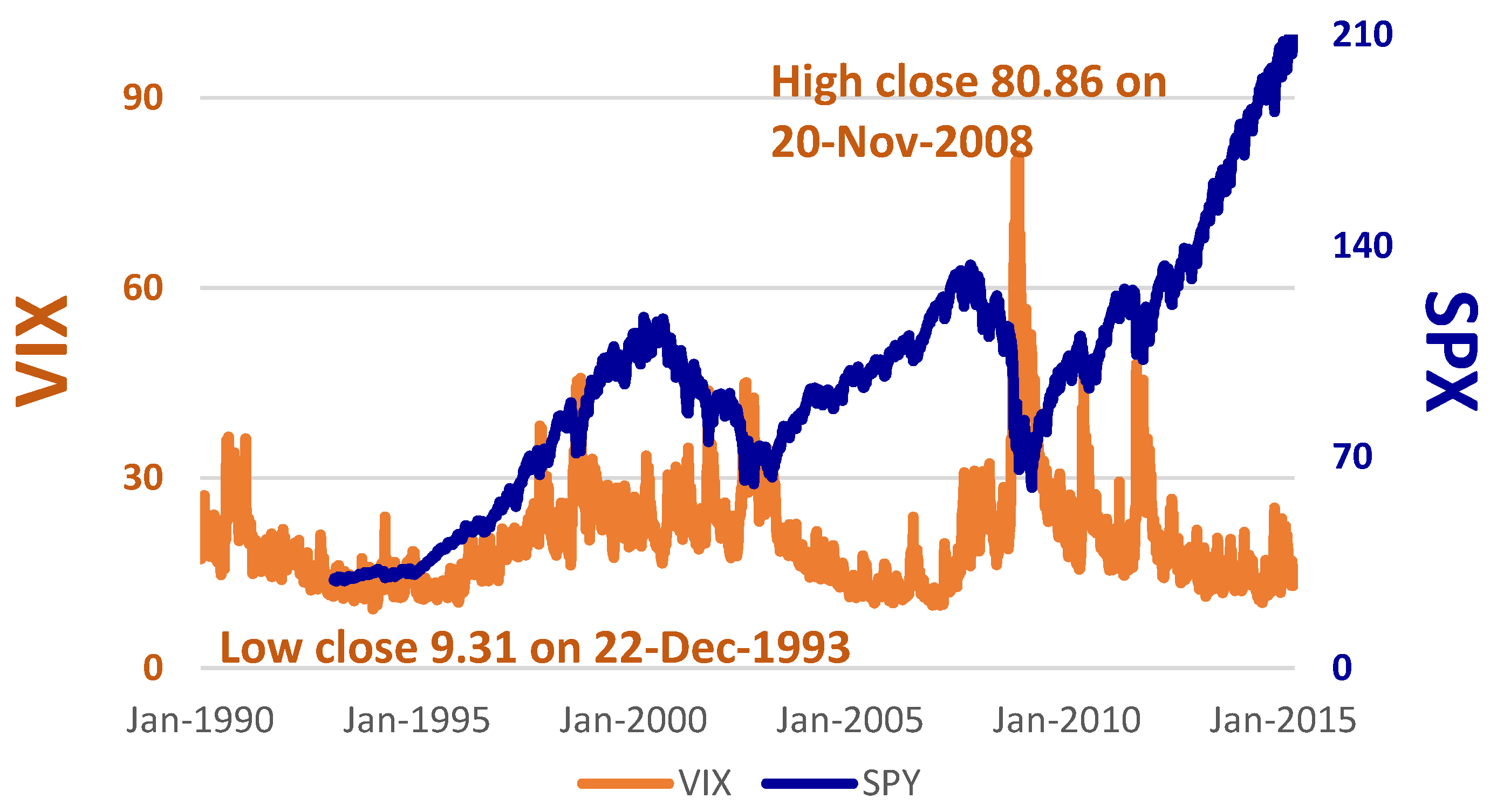
Figure 1 shows trends in S&P 500 and VIX for 1990–2014 and indicates that the highest point for VIX rises sharply from the beginning of September 2008 to its then highest historical level in November 2008, at 80.86. Asymmetric characteristics of VIX can also be observed. When the Global Financial Crisis (GFC) occurred in 2008–2009, VIX immediately reflected the panic on the part of market participants. As VIX was very high, this might have indicated that the market would rebound, and the stock price index would increase. History records that this did not happen quickly.

Previous studies have shown that the highly volatile market environment when VIX is at a peak can help predict future rises in the stock market index. When the market is highly volatile, the stock index falls along with the increase in VIX by more than the market, which is characterized by low volatility. This indicates that when the market is characterized by a highly volatile environment, the negative impact of VIX is relatively more severe (Giot 2005; Sarwar 2012).

Figure 1 shows an interesting phenomenon, namely when VIX rises rapidly, S&P 500 tends to fall simultaneously, which usually means that the index is not far from its lowest level. However, when VIX has already fallen to its lowest point and starts to rise again, and the stock market is bullish, the time for the market index to rebound is gradually approaching. Although trends in stock indexes do not always follow a certain course, and the prices and returns of financial derivatives such as futures and options are affected by current news and other technical indicators, the probability of investors predicting future trends in the index can be improved greatly by using VIX, so that risk management strategies are likely to be enhanced.

There have been numerous studies on VIX and market returns, with the focus primarily on the broader market index returns and discussing the ability of VIX to forecast option prices. VIX is an important market risk indicator that is used to predict future index volatility, especially in global markets with diversified portfolios, where investors cannot rule out the risk of changes in US stocks that might cause fluctuations in international stock markets. Using stock returns for the BRIC (Brazil, Russia, India and China) countries, Sarwar (2012) found that VIX not only influenced US stock market index returns, but also had a significant influence on BRIC market indexes.

In recent years, there has been an expansion of a wide range of financial market indexes that have provided investors with information to understand the indexes of crude oil and other energy issues, gold, bonds, index strategies, social enterprises, high dividend yields, and low volatility, as well as a wide range of sub-indexes for various industries. However, while the indexes measure the performance of the markets, in the absence of trading on spot indexes, this has resulted in the generation of exchange-traded funds and many other financial derivatives (for a critical econometric analysis of financial derivatives, see (Chang and McAleer 2015)).

ETFs use the “index” as a benchmark, selecting the constituent parts as investment targets, to replicate the market index performance. Although ETF is referred to as a fund, it is different from the typical definition of a fund. The term “fund” usually refers to an open-end mutual fund and is different in nature from an ETF. A mutual fund is part of an actively managed investment portfolio, but an ETF is a passively managed fund.

Furthermore, if the investor wants to buy or sell a mutual fund, it can only be redeemed with the asset management company that issued the mutual fund, according to the net worth of the fund at the close of the day on which it was traded. The ETF is traded at the listed price and can be traded directly with other investors using market prices.

As ETF replicates the performance of the broader market index, unless there is a change in the constituent parts of the index that is tracked, fund managers will not access the market frequently, so there will typically be few changes made to ETF portfolios. The securities brokerage fees that need to be paid for funds will be reduced significantly compared with actively managed funds and will become another feature of passively managed funds that attracts investors.

It has been found in practice that returns on mutual funds are frequently lower than the average returns for the market. It is seldom the case that mutual funds can continue to beat the market and remain sufficiently stable to earn excess profits. In other words, when compared with market funds for which the stocks are selected based on active strategies, ETFs that track the market index are more profitable. If their low management fees are also taken into consideration, the greater will be the gap between the two in terms of profitability.

Europe is an important economic and financial region, and a single country’s market index reflects that region’s economic performance, such as the Financial Times Stock Exchange index (FTSE100), which consists of 100 stocks that are traded on the London Stock Exchange. The 100 stocks are primarily those of major British companies, but also include a small number of companies from nine other European countries.

Since 1988, CAC40 has comprised the 40 largest listed companies’ stocks traded on the Paris Bourse. DAX comprises 30 selected blue-chip companies whose shares are traded on the Frankfurt Stock Exchange. Besides being calculated based on market value, DAX is also determined by attaching weights to the 30 stocks based on expected dividends. FTSE100, CAC40 and DAX are the indexes of economic performance that reflect the three major European capital markets, UK, France, and Germany, respectively, and have important roles to play in enabling investors to understand the dynamics of the European economies.

Unlike single-country stock indexes that consist of the stocks listed on specific stock exchanges, regional indexes to which relatively large numbers of market participants currently pay attention are MSCI Europe Index, EURO STOXX50, and MSCI Europe Union. The compilation of regional indexes is arbitrary, so that it is necessary to examine the approach used by the index issuing companies. For example, EURO STOXX50 selects only 50 weighted stocks from among all European industries, whereas MSCI Europe consists of 500 stocks.

Although selecting a larger number of stocks means that the respective index will embody the characteristics of regional industries, this dilutes the impact of the industry shares on the overall index. Therefore, the kind of index that best represents the economic performance in Europe will be decided by market participants. Moreover, the MSCI series of European regional indexes consists of almost ten different indexes, the differences between them being relatively small. Thus, when investors refer to European stock markets, they will usually first observe EURO STOXX50, and thereby examine the overall performance of European stock markets.

EURO STOXX50 comprises 50 blue-chip stocks from various industries within Europe, with 12 European countries being covered by the stocks. Derivative financial products related to EURO STOXX50 include futures, options and ETFs that track EURO STOXX50 which, together with ETF, can depict the overall trend of European markets.

The expectation of ETF is to earn the same return as the market index, but investors must still decide when to buy and sell ETF to realize a gain or loss. When implementing a trading strategy, if institutional or individual investors can fully understand the market index being tracked by ETF, it may then be possible to reduce investment risk.

Although ETF is a derivative financial commodity that has become widely available within the last decade, previous research does not seem to have performed any serious statistical analysis of ETF returns in comparison with VIX. A primary purpose of the paper is to investigate the extent to which US stock market risk indicators affect European markets, and to compare the similarities and differences between ETFs issued by a single country and market indexes, as well as ETFs for Europe that are influenced by VIX.

To reduce any possible biases in the calculation of standard errors, the paper uses the Diagonal BEKK multivariate conditional volatility model to adjust for conditional heteroskedasticity so that a robust comparison of the empirical results can be drawn.

The remainder of the paper proceeds as follows. The VIX literature is reviewed briefly in Section 2. Descriptions of the sample and variables are in Section 3, followed by the empirical results in Section 4, and concluding remarks in Section 5. The VAR(p) and Diagonal BEKK models are discussed in the Appendix A and Appendix B.

2. VIX Literature Review

Sarwar (2012) uses US stock data for 1993–2007 and finds that VIX and US stock market returns are negatively correlated. Moreover, the negative relationship is especially significant when the US stock market is characterized by high volatility. Sarwar (2012) also examines the impact of VIX on market returns of four BRIC countries and finds that a significant negative relationship exists between VIX and the Chinese and Brazilian stock markets, with the negative relationship being particularly strong when the Brazilian stock market is experiencing high volatility. However, there was apparently no negative relationship between VIX and the Russian and Indian stock markets.

These empirical results suggest that the relationship between stock market returns and VIX is asymmetric (also Giot 2005). This paper confirms that VIX is not only applicable to the US stock market, but that it can also be used to explain movements in stock markets in other countries. Previous studies have used VIX to capture the impact of investor sentiment on stock returns. By separating market participants into institutional investors and individual investors, several studies have found that institutional investors tend to be more easily impacted by macroeconomic variables, financial ratios, and other related variables, and that VIX has a smaller impact on stock returns than macroeconomic variables and financial ratios (see Arik 2011; Fernandes et al. 2014).

In addition to the relationship between VIX and US stock market returns, Cochran et al. (2015) use fuel oil, gasoline and natural gas futures prices returns data for 1999–2013, and find that natural gas futures returns and changes in VIX are positively correlated. However, changes in VIX are negatively correlated for heating oil and gasoline, suggesting that the returns on natural gas, contrary to the returns on the other two commodities, are more able to withstand volatility in stock markets.

This phenomenon is particularly significant during the GFC of 2008–2009. The paper shows empirically that the impact of VIX returns is not limited to stock market returns, but that the index exerts considerable influence on the spot and futures price returns for heating oil, gasoline and natural gas.

There are currently many methods that are used to measure volatility, such as historical variance or standard deviation of observed returns. Such methods are exceedingly simple and static, meaning the risk measure does not incorporate any shocks that might change over time, so it is natural that they have inherent shortcomings. For example, the volatility of the returns on risky assets may be characterized by fat-tailed distributions, asymmetry, leverage, clustering, persistence, or mean reversion (see Poon and Granger 2003).

There are many methods used to measure risk in empirical research, such as historical volatility, implied volatility, expected volatility, VIX, conditional volatility, stochastic volatility, and realized volatility. The volatility measure that is the easiest to understand is historical volatility, which uses data on events that have already taken place to calculate volatility and is therefore regarded as a backward-looking index.

The other two indexes based on conditional and implied volatility may be explained simply, as follows:

2.1. Conditional Volatility

This approach reflects the fact that the conditional variance can change dramatically over time when high frequency data are used. Engle (1982) proposed an ARCH model which incorporated the heterogeneity of the conditional variance and volatility clustering of time series data to bring the model closer to reality. Bollerslev (1986) extended the ARCH model by proposing a generalized autoregressive conditional heteroskedasticity (GARCH) model to improve explanatory power.

GARCH includes two effects, namely the ARCH effect that captures the short-term persistence of returns shocks on conditional volatility, and the GARCH effect that contributes to the long-term persistence of returns shocks on conditional volatility. Tsay (1987) showed that the ARCH model could be derived from a random coefficient autoregressive process.

As the GARCH model is unable to capture the asymmetric effects of positive and negative shocks of equal magnitude on the subsequent conditional volatility, Glosten et al. (1993) modified (G)ARCH by including an indicator variable to distinguish between positive and negative shocks of equal magnitude. Numerous studies have found that the resulting GJR model has useful explanatory power in distinguishing between positive and negative shocks on the conditional volatility of daily stock returns (see, among others, Ling and McAleer 2003).

Nelson (1991) proposed the exponential GARCH (EGARCH) model. Besides capturing the asymmetric effect of the unexpected impact on the conditional variance, this model purports to capture the important leverage effect of shocks on the volatility of financial assets, based on the debt-equity ratio. Leverage refers to the outcome in which the effects of negative returns shocks on volatility are greater than those of positive shocks of equal magnitude.

McAleer (2005, 2014) analyzed GARCH and alternative conditional volatility models that incorporate asymmetry (see Black 1976), but not leverage, which was shown to be excluded from derivations that are based on the random coefficient autoregressive approach. For a detailed derivation and the statistical properties of the EGARCH model, see McAleer and Hafner (2014).

From a practical perspective, Kanas (2013) used the GARCH model to engage in out-of-sample forecasting in relation to the excess returns data for S&P500 index for 1990–20061. The empirical results indicated that the explanatory power of GARCH with VIX was better than GARCH without VIX, or just VIX.

Following the establishment of financial asset diversification and investment portfolios, several different multivariate conditional volatility models have been derived, such as the constant conditional correlation (CCC) model (Bollerslev 1990), dynamic conditional correlation model (Engle 2002), varying conditional correlation model (Tse and Tsui 2001), VARMA-GARCH model (Ling and McAleer 2003), and VARMA-AGARCH model (McAleer et al. 2009). For details on the asymptotic properties of the QMLE of GARCH models, see Boussama (2000).

2.2. Implied Volatility

As volatility is latent, the concept of implied volatility involves incorporating the specific strike price and the option price on the maturity date into an option pricing formula to infer indirectly or imply the volatility of the option. To derive implied volatility, it is necessary to use an appropriate option pricing model.

While the Black-Scholes option pricing model is widely used, a shortcoming is that it assumes the variance of the stock price returns is fixed, which does not accord with what is actually observed in markets, namely: (1) different levels of implied volatility are inherent in the strike price; and (2) implied volatility in-the-money and out-of-the-money is greater than the implied volatility at-the-money (also known as the implied volatility smile). Given this drawback, different evaluation models have been proposed, such as a binomial tree model to evaluate the proposed option price (see Cox et al. 1979; Dumas et al. 1998; Rosenberg 2000; Borovkova and Permana 2009).

Another implied or expected volatility measure is VIX, which was used by the CBOE in 1993 to serve as a market volatility thermometer. Prior to 2003, VIX was calculated by selecting S&P 100 index options based on the call and put options closest to the price level for the most recent month and the second month for a total of eight series. This involved reweighting the average of the indexes obtained after calculating their implied volatility.

As the trading volume of S&P 500 index options gradually increased, in 2003 the CBOE started to calculate VIX based on S&P 500 index option prices. The CBOE has retained, and continued to calculate and announce, the original VIX based on the S&P 100 index option prices, but changed the acronym to VXO.

VIX is calculated using all the closest at-the-money calls and put S&P500 index option premium prices in the most recent month and the second month to obtain indirectly the weighted average of the volatility series. VIX is an expected volatility series, with the integration process being model free. In early 2001, the COBE announced VXN, which uses the same method to calculate VIX, but is based on NASDAQ100 index options prices.

Previous studies have suggested that, although VIX is not necessarily able to predict accurately the returns variability, the information it provides serves as a valuable reference to investors, so that cannot be ignored when examining the risk-return relationship. Cochran et al. (2015) noted that the impact of VIX can be felt not only in the stock market, but also in returns in spot commodity and futures markets.

Furthermore, in previous empirical research on the correlation between VIX and market weighted returns, the focus of attention has primarily been on the market weighted returns and on investigating the ability of VIX as a proxy variable for volatility to forecast option prices. There seems to have been little or no research on the relationship between VIX and ETF returns for non-US market indexes. This is an omission that should be remedied as VIX not only influences the US stock market, but also affects international stock market returns.

ETF is a derivative financial product that has come to prominence during the last decade, and the volatility of returns on risk-based assets has increasingly drawn the attention of institutional and individual investors. How to use the information provided by the volatility of ETF to enable investors to achieve optimal risk management is of serious practical concern. This paper will examine the impact of US financial markets on European financial markets, and assess the extent to which ETF returns based on European market indexes have been influenced by VIX.

A discussion of the VAR(p) and Diagonal BEKK models for the empirical analysis is given in the Appendix A and Appendix B.

3. Data and Variables

This paper selects ETFs that track three major US stock indexes, SPY, DIA and ONEQ, as well as ETFs for three major European stock market indexes, FEZ, DBXD and XUKX. Daily closing prices for each ETF variable are sourced from Yahoo Finance, while VIX data are sourced from the CBOE website.

Table 1. Sample Periods.

	Endogenous Variables
Market	ETFs	Benchmark Index	Sample Time
US	SPY	S&P 500	29 January 1993~30 March 2015
	DIA	DJIA	20 January 1998~30 March 2015
	ONEQ	NASDAQ	1 October 2003~30 March 2015
Europe	FEZ	EURO STOXX50	21 October 2002~30 March 2015
	DBXD	German DAX	17 January 2007~30 March 2015
	XUKX	FTSE100	6 September~30 March 2015
	Exogenous variables
	VIX		2 January 1990~30 March 2015
	S&P 500		29 January 1993~30 March 2015

Data source: ETF Database, https://beta.finance.yahoo.com/ accessed 1 October 2015.

illustrates the indexes tracked by each ETF and sample periods. The endogenous variables include ETF daily returns, R, which are obtained as the logarithmic differences of daily closing prices, multiplied by 100.

We briefly introduce each ETF and the underlying tracked index. The method used to compile each index is based on the discretion of the issuing company, with the information conveyed by, and the meaning of each index being based on, the judgement of the user.

SPY refers to SPDR S&P 500 ETF, the world’s first ETF, listed on the New York Stock Exchange in 1993. As SPY was listed before any other ETF, the ETF’s accumulated net worth is the largest. SPY tracks S&P 500 composite index and is most able to represent US stock market performance. The stocks that comprise the index are selected from the largest 500 companies in terms of market value traded on the New York Stock Exchange and Nasdaq, and include Microsoft, Apple, P&G, Johnson & Johnson, Morgan Chase, IBM, Coca-Cola, AT&T and other leading companies.

DIA is SPDR Dow Jones Industrial Average ETF, which tracks the Dow Jones Industrial Average (DJIA). The index comprises 30 blue-chip stocks. Although it is referred to as an industrial index, the proportion allocated to the industrial sector falls far short of that at the end of 19th century, when the index was established, and reflects core transformations of the US economy. The DIA index is characterized by the compilation of an average weighted by prices, which differs from the typical indexes that are weighted by market capitalized values.

The highly priced stocks comprising the index which fluctuate less than the low-priced stocks have more of an impact on the DIA index, which is limited to 30 stocks. According to data at the close of trading on 22 May 2015, the top three industrial sectors in the DIA portfolio, ranked by weights, were industry 19.78%, IT industry 17.71%, and financial sector 16.76%. The DIA portfolio differed only slightly from the DJIA Average index that it tracked.

ONEQ is Fidelity Nasdaq Composite Index Tracking Stock Fund, which tracks the Nasdaq Composite Index. This comprises more than 5000 enterprises traded on Nasdaq and is calculated using the weighted market value. As the ONEQ stock portfolio is primarily comprised of large listed stocks that replicate market value, with the remaining part being selected using a sampling method, it can involve the selection of more than 5000 companies. As ONEQ is much larger than the other ETFs that track S&P 500 or DJIA ETFs, its portfolio does not replicate the Nasdaq index.

Data compiled after the close of trade on 22 May 2015 show that the fund is comprised of stocks for IT industry, at 46.17%, non-essential consumer goods accounting, 17.57 percent, and the health care industry, 16.92%. As for the Nasdaq Composite Index, the focus is in the performance of high-tech related industries.

This paper selects ETFs that track three major US stock market indexes, the intention being to examine their performance in terms of tracking each index. There are some differences between the three major market indexes in terms of the economic conditions in the US market. Investors generally believe that S&P 500 is most able to represent the overall economic performance of US capital markets because, when compared with the industries that comprise DJIA, S&P 500 is relatively broad. Although NASDAQ100 Composite Index is comprised of more stocks than the other two, as emphasis is placed on high-tech industry stocks. Investors see Nasdaq Composite as reflecting the performance of innovative technology and high-tech industries.

This paper selects ETFs that track the three major European stock market indexes, FEZ, DBXD and XUKX, of which FEZ tracks EURO STOXX50, which is an index that measure the performance of European industries. This is unlike DBXD and XUKX, which track indexes for single countries.

FEZ is SPDR EURO STOXX 50 ETF, which is the same as EURO STOXX50 in terms of portfolio selection. The underlying index consists of a total of 50 blue-chip stocks spread over 12 European countries. Data after the close of trade on 27 May 2015 showed the three leading industrial sectors comprising FEZ were the financial sector at 26.53%, non-essential consumer goods at 11.33%, and industry at 11.03%. There was only a slight difference between FEZ and the underlying tracked EURO STOXX50.

DBXD ETF is db x-trackers DAX^® UCITS ETF, which tracks DAX, which is used to measure the performance of the German stock market and comprises 30 blue-chip stocks traded on the Frankfurt Stock Exchange. In addition to using the weighted market value, consideration is given to the stock index’s constituent parts to determine expected dividends. The DBXD portfolio consists of 30 blue-chip stocks and is traded in Euro. From the listing of DBXD in 2007 to the first quarter of 2015, the rate of return has been 71.68%. Differences between the rates of return for DBXD and DAX over the same period are quite small.

XUKX is the db x-trackers FTSE 100 UCITS ETF, which tracks FTSE 100, comprising 100 leading large stocks in terms of market value traded on the London Stock Exchange. Although FTSE 100 is used to measure the performance of the UK stock market, as the London Stock Exchange is Europe’s financial center, there is no shortage of companies from other European countries whose stocks are listed and traded. XUKX has similar characteristics to FTSE 100 for stocks that comprise its portfolio, with Royal Dutch Shell of The Netherlands, for example, accounting for a 4.62% share.

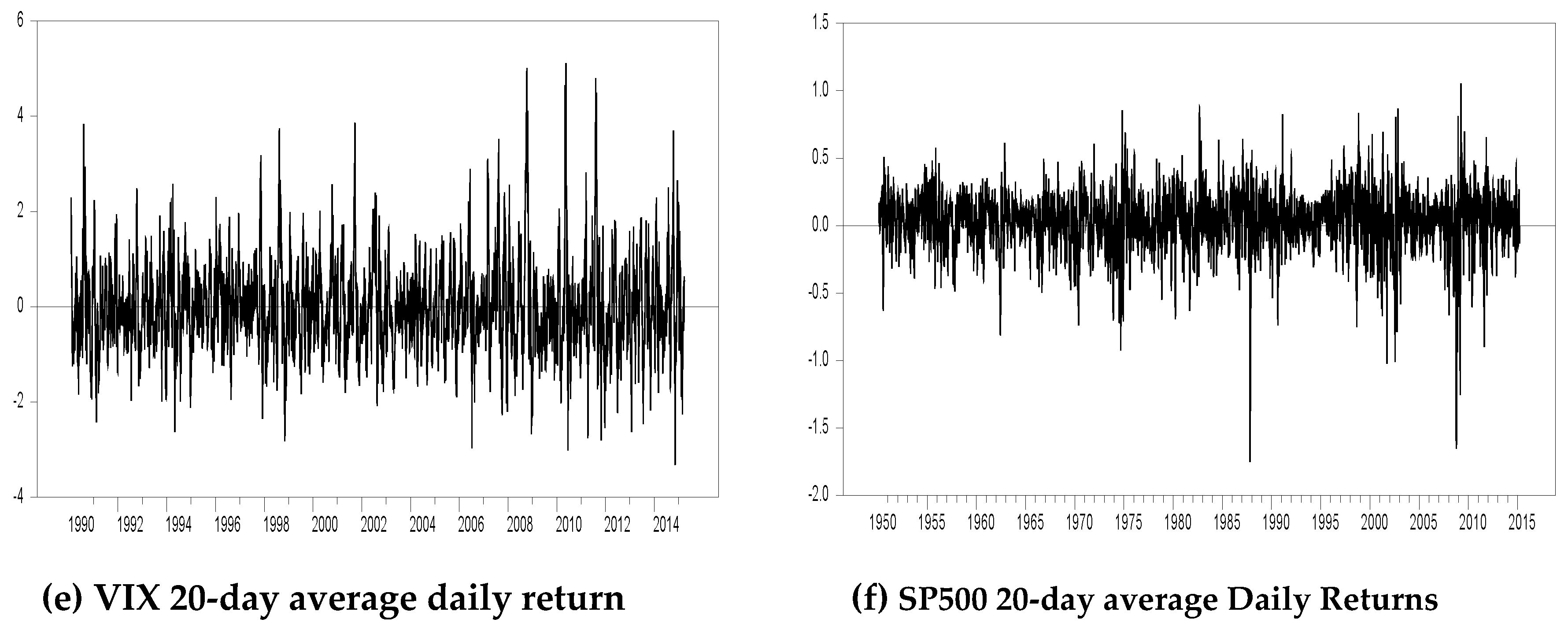
VIX data are sourced from CBOE. According to Fernandes et al. (2014), VIX is characterized by long-term dependency, so this paper uses 10-day and 20-day moving averages for VIX returns, R_VIX, denoted as R10_VIX and R20_VIX, respectively, to analyze whether average VIX for different time periods, such as during the previous 10 and 20 days, affects ETF returns.

For European investors, S&P 500 best represents the performance of the US stock market. The return on S&P 500, given as R_SP500, is another exogenous variable. For this reason, the 10- and 20-day moving averages, R10_SP500 and R20_SP500, respectively, are used to examine whether S&P 500 returns for different periods have an impact on ETF returns. 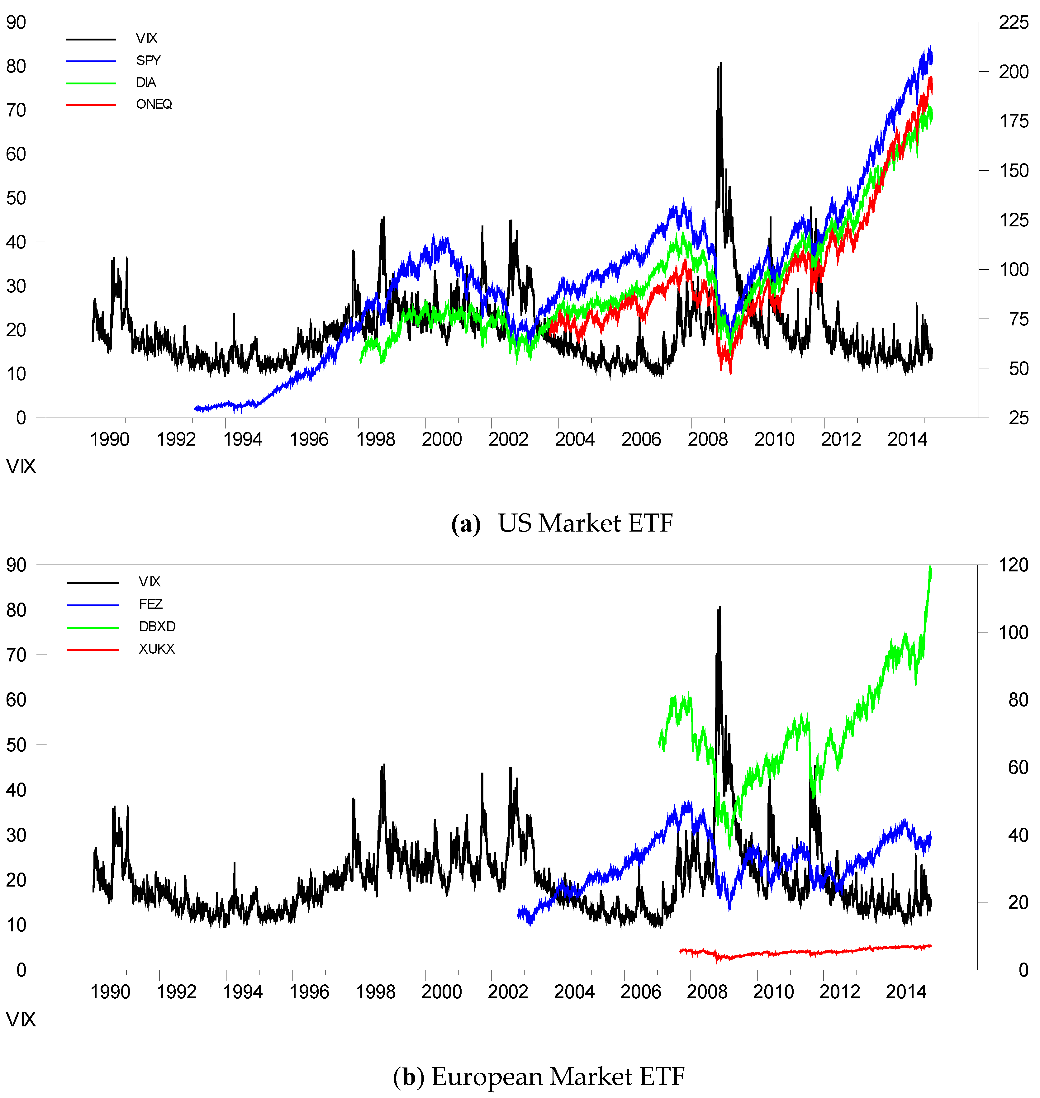From the range of the coordinates on the vertical axes in Figure 2, we can see that using moving averages reduce variations in the series. From Figure 3, VIX exhibits a negative relationship with both ETF for the USA and ETFs for European markets.

Table 2. Sample Statistics.

Endogenous Variables
	USA			Europe
ETF	R_SPY	R_DIA	R_ONEQ	R_FEZ	R_DBXD	R_XUKX
Mean	0.034	0.025	0.036	−0.005	0.023	0.013
Median	0.038	0.033	0.082	0.000	0.036	0.000
Maximum	13.558	12.710	10.022	16.169	11.148	13.840
Minimum	−10.364	−9.874	−8.181	−12.142	−8.038	−21.575
Std. Dev.	1.175	1.294	1.409	2.052	1.473	1.521
Skewness	−0.107	0.386	−0.200	−0.008	−0.098	−2.221
Kurtosis	13.585	17.709	8.336	9.355	8.603	47.260
Exogenous variables
	R_VIX	R_S&P500
Mean	−0.025	0.017
Median	−0.323	0.036
Maximum	40.547	10.957
Minimum	−35.059	−9.470
Std. Dev.	7.028	1.403
Skewness	0.595	−0.305
Kurtosis	6.198	12.635

presents descriptive statistics for the variables. ETF, which tracks the index, has many values that are close to, but not identical, to those of the index. This arises because a certain percentage of the financial products of the asset management company that issues ETFs to track underlying indexes are similar to those of the market. It is standard for 80% of such stocks to be the same, though the actual proportion depends on what is disclosed in the ETF prospectus. The asset management company issuing ETFs retains the right, based on the principle of passively managing ETFs, to manage independently any excess amounts.

If the skewness coefficient is positive, most of the observations in the sample are lower than the average of the sample values. On the contrary, if the skewness coefficient is negative, most of the observations in the sample are greater than average. If kurtosis exceeds 3, this indicates a distribution that has a higher peak and wider tails as compared with a normal distribution.

Unit root tests of the endogenous and exogenous variables are summarized in

Table 3. Unit Root Tests.

ADF Test
Market	Variables	Trend and Intercept	Intercept Only	No Trend or Intercept
US	R_SPY	−58.106 ***	−58.106 ***	−58.029 ***
	R_DIA	−72.456 ***	−72.462 ***	−72.430 ***
	R_ONEQ	−57.239 ***	−57.233 ***	−57.195 ***
Europe	R_FEZ	−63.167 ***	−63.168 ***	−63.161 ***
	R_DBXD	−45.995 ***	−45.968 ***	−45.963 ***
	R_XUKX	−54.310 ***	−54.302 ***	−54.311 ***
	R_VIX	−7.659 ***	−7.636 ***	−2.847 ***
	R_SP500	−127.464 ***	−127.467 ***	−127.362 ***
PP Test
Market	Variables	Trend and Intercept	Intercept Only	No Trend or Intercept
US	R_SPY	−82.507 **	−82.505 **	−82.211 **
	R_DIA	−73.122 **	−73.124 **	−73.002 **
	R_ONEQ	−57.418 **	−57.403 **	−57.355 **
Europe	R_FEZ	−63.660 **	−63.655 **	−63.576 **
	R_DBXD	−46.041 **	−46.008 **	−46.000 **
	R_XUKX	−55.659 **	−55.528 **	−55.526 **
	R_VIX	−6.001 **	−5.984 **	−2.005 *
	R_SP500	−127.477 ***	−127.480 ***	−127.353 ***

Note: ***, ** and * denote significance at 1%, 5%, and 10%, respectively.

. The Augmented Dickey-Fuller (ADF) and Phillips-Perron (PP) tests are used to test for unit roots in returns. ADF accommodates serial correlation by specifying explicitly the structure of serial correlation in the error, but the non-parametric PP test allows mild assumptions that do not assume a specific type of serial correlation and heteroskedasticity, and can have higher power than ADF under a wide range of circumstances.

The null hypothesis of the ADF and PP tests is that the series have a unit root (Dickey and Fuller 1979; Phillips and Perron 1988). In Table 3, based on the ADF and PP tests, the large negative values in all cases indicate rejection of the null hypothesis at 1%, which suggests that the ETF returns are stationary.

4. Empirical Results

Table 4. Europe Market ETF and VIX VAR.

Variables	R_FEZ	R_DBXD	R_XUKX
R_FEZ(−1)	−0.083 *	0.117 **	0.173 **
	(0.039)	(0.027)	(0.027)
R_DBXD(−1)	0.097	−0.068	0.018
	(0.056)	(0.040)	(0.039)
R_XUKX(−1)	−0.035	−0.132 **	−0.392 **
	(0.045)	(0.032)	(0.031)
C	−0.006	0.025	0.017
	(0.046)	(0.032)	(0.032)
R_VIX(−1)	0.020	−0.021 **	−0.026 **
	(0.009)	(0.007)	(0.006)
R10_VIX(−1)	0.049	−0.016	−0.054 *
	(0.037)	(0.026)	(0.026)
R20_VIX(−1)	−0.038	−0.049	−0.006
	(0.055)	(0.039)	(0.039)

Note: ** and * denote significance at 1% and 5%, respectively. Standard errors are in parentheses.

and

Table 5. Europe Market ETF and S&P 500 VAR.

Variables	R_FEZ	R_DBXD	R_XUKX
R_FEZ(−1)	−0.047	−0.038	−0.064
	(0.052)	(0.037)	(0.035)
R_DBXD(−1)	0.104	−0.050	0.042
	(0.056)	(0.039)	(0.038)
R_XUKX(−1)	−0.031	−0.145 **	−0.415 **
	(0.045)	(0.032)	(0.031)
C	−0.001	0.020	0.007
	(0.046)	(0.032)	(0.031)
R_SP500(−1)	−0.137 **	0.346 **	0.502 **
	(0.069)	(0.049)	(0.047)
R10_SP500(−1)	−0.332	−0.006	0.228
	(0.176)	(0.124)	(0.120)
R20_SP500(−1)	0.135	0.071	−0.145
	(0.246)	(0.172)	(0.167)

Note: ** denote significance at 1%. Standard errors are in parentheses.

report the dynamic relationships among three ETFs, as well as the effects of exogenous variables, VIX on ETF returns, for the European market. To examine short- and long-terms effects of VIX on ETF returns, we incorporate the single day VIX rate of change (followed by S&P 500), 10-day average VIX rate of change (followed by the S&P 500 index), and 20-day average VIX rate of change (followed by S&P 500 index) in alternative models. In

Table 6. US Market ETF and VIX VAR.

Variables	R_DIA	R_ONEQ
R_DIA(−1)	−0.139 **	0.035
	(0.039)	(0.044)
R_ONEQ(−1)	0.052	−0.087 *
	(0.034)	(0.039)
C	0.033	0.038
	(0.020)	(0.023)
R_VIX(−1)	0.002	−0.004
	(0.005)	(0.005)
R10_VIX(−1)	0.027	0.019
	(0.018)	(0.020)
R20_VIX(−1)	−0.019	−0.027
	(0.026)	(0.030)

Note: ** and * denote significance at 1% and 5%, respectively. Standard errors are in parentheses.

, we replace VIX returns with S&P 500 returns as an exogenous variable and compare their respective effects.

4.1. ETFs in the European Market

Table 4 reports the results of estimating VAR on returns of the European market ETFs, FEX, DBXD, and XUKX, that track the underlying indexes for EURO STOXX50 INDEX, DAX, and FTSE 100, respectively.

The returns for the three European ETFs in the previous period are significantly negatively correlated with the returns in the current period, where the negative impact of returns of XUKX in the previous period on those in the current period is the greatest, at −0.392. ETF returns which tracked different indicators were characterized by mutual dynamics: for VAR, FEZ returns lagged one period were significant in explaining returns of the other two ETFs.

FEZ returns lagged one period had a significant positive influence on DBXD returns in the current period, at 0.117, and had a significant positive influence on XUKX returns in the current period, at 0.173. However, XUKX returns lagged one period only significantly explained DBXD returns in the current period, at −0.132.

Thus, FEZ returns had significant explanatory power for returns in the current period of the other two ETFs that tracked a single country index, as the source of the stocks comprising FEZ was EURO STOXX50 INDEX, an index of European markets. It is relatively easy to select large-valued stocks from the same industries as those for DBXD and XUKX, which were correlated through respective ETF returns.

The negative impact of VIX rates of change on returns to XUKX ETF are both significant and persistent, while the returns of FEZ are the least affected by VIX rates of change. The single day rate of change in VIX in the previous period has a significant negative impact on returns of XUKX in the current period, at −0.026. The 10-day average rate of change in VIX also had a significant negative impact on the return of XUKX in the current period, at −0.054.

However, when the moving average increases from 10 to 20 days, the 20-day moving average VIX rates of return do not have a significant impact on the return of XUKX in the current period. The rate of change in VIX in the previous period has a significant negative impact on the return of DBXD in the current period, at −0.021, but it is not impacted by the 10-day or 20-day average VIX rate of change. Moreover, the coefficients of VIX are negative, indicating that when the rate of change in VIX is large, this will result in a reduction in the returns on DBXD and XUKX in the following period.

The returns of ETFs that track a single country stock index tend to be influenced relatively more by the rate of change in VIX than the Euro stock market, but the impact of the VIX rate of change ETF returns remains temporary.

Table 5 reports the counterpart results with the daily, 10-day and 20-day average rate of change in the returns of S&P500 on returns of the three European ETFs. The empirical results show that the rates of change in S&P500 have negative and significant impacts on FEZ returns, while there is a positive and significant impact on the returns of both DBXD and XUKX.

The single day rate of change in S&P500 in the previous period has a significant positive impact on XUKX returns in the current period, at 0.502. The 10-day average VIX rate of change shows a less significant positive impact on XUKX returns, at 0.228. However, when the period of the moving average is extended from 10 to 20 days, the 20-day average rate of change in S&P 500 does not have a significant impact on the XUKX return in the current period.

The rate of change in S&P500 in the previous period has a significant positive impact on the DBXD return in the current period, at 0.346, but DBXD is not impacted by the 10-day or 20-day average rate of change in S&P500. Moreover, the coefficients of S&P500 are positive, indicating that larger positive returns in S&P500 in the current period will cause an increase in subsequent returns on DBXD and XUKX.

4.2. ETFs in the US Market

Table 6 reports the results of VAR on the returns of the two US market ETFs, DIA and ONEQ, that track the underlying indexes for DJIA and Nasdaq Composite. However, as VIX is based on call and put S&P500 index option premium prices to obtain indirectly the weighted average of the implied volatility series, we exclude SPY that tracks the underlying indexes for S&P500 from the VAR system for the US market to reduce the problem of possible measurement error.

The returns for the two US ETFs in the previous period are significantly negatively correlated with returns in the current period, where the negative impact of the returns of DIA in the previous period on those in the current period is the greatest, at −0.145. However, there are no significant mutual dynamics in VAR, with DIA returns lagged one period having no impact on the returns of ONEQ ETFs, and vice versa.

The single day rate of change in VIX in the previous period has no impact on the return of DIA in the current period. Similarly, there is no impact from either the 10-day or 20-day average VIX rate of change on DIA returns in the current period. Moreover, the single day VIX rate of change in the previous period, and both the 10-day and 20-day average VIX rates of change have no significant impact on ONEQ in the current period.

4.3. Testing and Correcting for Conditional Heteroskedasticity

The results of multivariate ARCH-LM tests are given in

Table 7. ARCH-LM Tests for European and US Market ETF Returns.

Europe	${\widehat{\mathsf{\epsilon }}}_{R\_\mathrm{FEZt}}$	${\widehat{\mathsf{\epsilon }}}_{R\_DBXDt}$	${\widehat{\mathsf{\epsilon }}}_{R\_XUKXt}$
LM statistic	38.819 *	28.254 *	321.64 *
	(0)	(0)	(0)
US	${\widehat{\mathsf{\epsilon }}}_{R\_DIAt}$	${\widehat{\mathsf{\epsilon }}}_{R\_ONEQt}$
LM statistic	97.495 *	129.692 *
	(0)	(0)

Note: * denotes significance at the 1% level. p-values are in parentheses.

, which show the shocks of returns of ETFs significantly reject the null hypothesis that $B_1$ is equal to zero at 1%.

Table 8. Mean Equation for European Market ETF and VIX (whole period) (10 September 2007 to 30 March 2015).

Variables	R_FEZ	R_DBXD	R_XUKX
R_FEZ(−1)	−0.218 ***	−0.005	−0.038 **
	(0.031)	(0.023)	(0.019)
R_DBXD(−1)	0.183 ***	0.010	−0.045 *
	(0.038)	(0.026)	(0.021)
R_XUKX(−1)	0.019	−0.085 **	−0.080 **
	(0.037)	(0.021)	(0.020)
CONSTANT	0.063 ***	0.087 ***	0.083 ***
	(0.024)	(0.024)	(0.019)
R_VIX(−1)	0.000	−0.028 ***	−0.037 ***
	(0.006)	(0.004)	(0.004)
R10_VIX(−1)	−0.003	−0.017	−0.032 **
	(0.024)	(0.019)	(0.015)
R20_VIX(−1)	0.057	−0.039	0.046 *
	(0.037)	(0.031)	(0.025)

Note: ***, ** and * denote significance at 1%, 5% and 10%, respectively. Standard errors are in parentheses.

and

Table 9. Diagonal BEKK for Europe Market ETF returns (whole period) (10 September 2007 to 30 March 2015).

Variables	C			A	B
R_FEZ	0.263 ***			0.275 ***	0.951 ***
	(0.023)			(0.013)	(0.004)
R_DBXD	0.173 ***	0.176 ***		0.292 ***	0.940 ***
	(0.017)	(0.010)		(0.014)	(0.004)
R_XUKX	0.246 ***	0.139 ***	0.000	0.499 ***	0.859 ***
	(0.021)	(0.023)	(0.059)	(0.017)	(0.008)

Note: *** denote significance at 1%. Standard errors are in parentheses.

report the results of the estimation of VAR on three returns of the European ETFs by using the Diagonal BEKK model to correct for the conditional heteroscedasticity, with Table 8 and Table 9 presenting the results for VAR and Diagonal BEKK for the full sample period, 10 September 2007 to 30 March 2015.

The single day VIX rate of change in the previous period has a significant negative impact on the return of XUKX in the current period, at −0.037. The 10-day average VIX rate of change also has a significant negative impact on the return of XUKX in the current period, at −0.032. The rate of change in VIX in the previous period has a significant negative impact on the return of DBXD in the current period, at −0.028, but it is not impacted by the 10-day or 20-day average VIX rates of change. However, the VIX rates of change have no significant impact on FEZ returns in the current period. Overall, R_XUKX seems to have the best fit in terms of statistical significance of the estimated coefficients.

The results in Table 8 and Table 9 are presented for the full sample period for the European market (10 September 2007 to 30 March 2015). It is worth examining whether the quantitative and qualitative results were similar or drastically different for the sub-sample periods before, during and after the GFC, namely Before GFC (10 September 2007 to 30 March 2015), During GFC (1 November 2007 to 31 March 2009), and After GFC (1 April 2009 to 30 March 2015). There are few observations Before GFC, so the estimates should be treated with caution.

Table 10. Mean Equation for European Market ETF and VIX (Before GFC) (10 September 2007 to 30 October 2007).

Variables	R_FEZ	R_DBXD	R_XUKX
R_FEZ(−1)	−0.034 ***	0.201 ***	−0.198 ***
	(0.008)	(0.010)	(0.001)
R_DBXD(−1)	0.179 ***	−0.085 ***	0.454 ***
	(0.032)	(0.008)	(0.003)
R_XUKX(−1)	0.072 ***	−0.106 ***	−0.365 ***
	(0.019)	(0.003)	(0.002)
CONSTANT	0.784 ***	0.353 ***	0.804 ***
	(0.018)	(0.009)	(0.002)
R_VIX(−1)	0.028 ***	−0.010 ***	−0.033 ***
	(0.003)	(0.001)	(0.000)
R10_VIX(−1)	−0.018	−0.022 **	−0.012 ***
	(0.021)	(0.007)	(0.003)
R20_VIX(−1)	0.523 ***	0.236 ***	0.502 ***
	(0.021)	(0.010)	(0.008)

Note: *** and ** denote significance at 1% and 5%, respectively. Standard errors are in parentheses.

and

Table 11. Diagonal BEKK for Europe Market ETF returns (Before GFC) (10 September 2007 to 30 October 2007).

Variables	C			A	B
R_FEZ	1.022 ***			−0.311 ***	−0.000
	(0.024)			(0.013)	(0.000)
R_DBXD	0.418 ***	0.383 ***		−0.308 ***	−0.000
	(0.024)	(0.019)		(0.022)	(0.000)
R_XUKX	0.964 ***	0.491 ***	−0.000	0.511 ***	0.000
	(0.033)	(0.025)	(0.00)	(0.023)	(0.000)

Note: *** denotes significance at 1%. Standard errors are in parentheses.

report the estimates of the Mean Equation and Diagonal BEKK for the European Market ETF returns Before GFC,

Table 12. Mean Equation for European Market ETF and VIX (During GFC) (1 November 2007 to 31 March 2009).

Variables	R_FEZ	R_DBXD	R_XUKX
R_FEZ(−1)	−0.266 **	−0.078	0.030
	(0.083)	(0.058)	(0.059)
R_DBXD(−1)	0.280 **	0.053	0.081
	(0.106)	(0.080)	(0.072)
R_XUKX(−1)	−0.058	−0.152 *	−0.254 **
	(0.085)	(0.063)	(0.070)
CONSTANT	−0.193 *	–0.133 *	−0.110 *
	(0.078)	(0.058)	(0.060)
R_VIX(−1)	0.011	−0.021	−0.047 **
	(0.020)	(0.016)	(0.017)
R10_VIX(−1)	−0.090	−0.088	−0.092
	(0.083)	(0.074)	(0.071)
R20_VIX(−1)	0.065	−0.035	0.003
	(0.111)	(0.100)	(0.094)

Note: ** and * denote significance at 5% and 10%, respectively. Standard errors are in parentheses.

and

Table 13. Diagonal BEKK for Europe Market ETF returns (During GFC) (1 November 2007 to 31 March 2009).

Variables	C			A	B
R_FEZ	0.427 **			0.383 **	0.918 **
	(0.024)			(0.013)	(0.000)
R_DBXD	0.402 **	0.295 **		0.278 **	0.928 **
	(0.024)	(0.019)		(0.022)	(0.000)
R_XUKX	0.576 **	0.371 **	−0.000	0.485 **	0.837 **
	(0.033)	(0.025)	(0.00)	(0.023)	(0.000)

Note: ** denote significance at 5%. Standard errors are in parentheses.

report the estimates of the Mean Equation and Diagonal BEKK for the European Market ETF returns During GFC, and

Table 14. Mean Equation for European Market ETF and VIX (After GFC) (1 April 2009 to 30 March 2015).

Variables	R_FEZ	R_DBXD	R_XUKX
R_FEZ(−1)	−0.184 ***	−0.004	−0.037 *
	(0.035)	(0.026)	(0.020)
R_DBXD(−1)	0.153 ***	–0.001	–0.057 **
	(0.047)	(0.035)	(0.030)
R_XUKX(–1)	0.049	–0.073 **	–0.054 *
	(0.045)	(0.031)	(0.028)
CONSTANT	0.089 **	0.102 ***	0.087 ***
	(0.032)	(0.023)	(0.018)
R_VIX(−1)	−0.000	−0.030 ***	−0.038 ***
	(0.006)	(0.005)	(0.004)
R10_VIX(−1)	0.009	−0.010	−0.026 **
	(0.020)	(0.015)	(0.012)
R20_VIX(−1)	0.057	−0.036	0.050 **
	(0.033)	(0.024)	(0.020)

Note: ***, ** and * denote significance at 1%, 5% and 10%, respectively. Standard errors are in parentheses.

and

Table 15. Diagonal BEKK for Europe Market ETF returns (After GFC) (1 April 2009 to 30 March 2015).

Variables	C			A	B
R_FEZ	0.271 ***			0.243 ***	0.954 ***
	(0.023)			(0.013)	(0.004)
R_DBXD	0.215 ***	0.186 ***		0.287 ***	0.928 ***
	(0.023)	(0.012)		(0.020)	(0.007)
R_XUKX	0.287 ***	0.090 ***	0.000	0.504 ***	0.834 ***
	(0.022)	(0.031)	(0.048)	(0.020)	(0.013)

Note: *** denote significance at 1%. Standard errors are in parentheses.

report the estimates of the Mean Equation and Diagonal BEKK for the European Market ETF returns After GFC.

The estimates of the diagonal elements of the weight matrix A in Table 9 are all statistically significant, with the estimates of $a_{11}$, $a_{22}$ and $a_{33}$ being 0.275, 0.292 and 0.499, respectively. The estimates of the dynamic contributions to long run volatility, namely $b_{11}$, $b_{22} \mathrm{and} b_{33}$ are highly significant at 0.951, 0.94 and 0.859, respectively.

The estimated mean equations Before GFC, During GFC and After GFC are given in Table 10, Table 12 and Table 14, respectively. Most of the lagged effect are statistically significant for all three variables Before GFC, the lagged effects are sporadically significant for all three variables During GFC, and several lagged effects are statistically significant After GFC, especially for R_XUKX.

Table 10, Table 12 and Table 14 show the estimated Diagonal BEKK effects Before GFC, During GFC and After GFC, respectively. The estimates of $a_{11}$ and $a_{22}$ are negative for Before GFC, but the estimates should be viewed cautiously as the numbers of observations are too small for the short sample size. Nevertheless, the estimate of $a_{33}$ is very close to that in Table 9 at 0.511. The estimates of $b_{11}$, $b_{22} \mathrm{and} b_{33}$ are shown as 0, but this is because lagged effects cannot be estimated accurately with such few observations.

The estimate of $a_{11}$ in Table 13 During GFC differs from that in Table 9, but the estimates of $a_{22}$ and $a_{33}$ are very similar to their counterparts in Table 9 at 0.278 and 0.485, respectively. The estimates of $b_{11}$, $b_{22} \mathrm{and} b_{33}$ are very similar to their counterparts in Table 9 at 0.918, 0.928 and 0.837, respectively.

The estimates of $a_{11}$, $a_{22}$ and $a_{33}$ in Table 15 After GFC are very close to their counterparts in Table 9 at 0.243, 0.287 and 0.504, respectively, while the estimates of $b_{11}$, $b_{22} \mathrm{and} b_{33}$ are also very similar to their counterparts in Table 9 (as well as in Table 13) at 0.954, 0.928 and 0.834, respectively.

In summary, the estimates of the mean equations for the European markets tend to differ between the whole sample period and the sub-periods Before GFC, During GFC and After GFC. Except for the Before GFC, where the numbers of observations are insufficient for the asymptotic properties to be shown as adequate, the estimates of the matrices A and B in the Diagonal BEKK model are very similar for the whole sample period and the sub-periods During GFC and After GFC.

The empirical results show that the VIX rate of change in the previous period has no impact on the returns of ETFs in the US market, as VIX and the lagged market index ETFs are highly correlated due to overlapping information sets. There are only two significant lagged effects for R_DIA, whereas there are three significant lagged effects for R_ONEQ.

The estimates of the diagonal elements of the weight matrix A in Table 17 are both statistically significant, with the estimates of $a_{11}$ and $a_{22}$ being 0.2769 and 0.229, respectively. The estimates of the dynamic contributions to long run volatility, namely $b_{11}$ and $b_{22}$ are highly significant at 0.949 and 0.964, respectively.

Table 16. Mean Equation for US Market ETF and VIX (whole period) (3 October 2003 to 30 March 2015).

Variables	R_DIA	R_ONEQ
R_DIA(−1)	0.041	0.128 **
	(0.035)	(0.043)
R_ONEQ(−1)	−0.044 *	−0.117 ***
	(0.024)	(0.031)
CONSTANT	0.064 ***	0.076 ***
	(0.013)	(0.016)
R_VIX(−1)	0.001	−0.006
	(0.003)	(0.004)
R10_VIX(−1)	0.010	0.006
	(0.011)	(0.014)
R20_VIX(−1)	0.009	0.010
	(0.018)	(0.022)

Note: ***, ** and * denote significance at 1%, 5% and 10%, respectively. Standard errors are in parentheses.

and

Table 17. Diagonal BEKK for US Market ETF returns (whole period) (3 October 2003 to 30 March 2015).

Variables	C		A	B
R_DIA	0.138 ***		0.269 ***	0.949 ***
	(0.010)		(0.012)	(0.005)
R_ONEQ	0.126 ***	0.071 ***	0.229 ***	0.964 ***
	(0.010)	(0.008)	(0.011)	(0.003)

Note: *** denote significance at 1%. Standard errors are in parentheses.

report the results of estimating VAR on the three returns of ETFs in the US market by using Diagonal BEKK, with Table 16 and Table 17 presenting the results of VAR and Diagonal BEKK, respectively, for the full sample period (3 October 2003 to 30 March 2015). As in the case of the European market, it is worth examining whether the quantitative and qualitative results were similar or drastically different for the sub-sample periods before, during and after the GFC, namely Before GFC (3 October 2003 to 30 October 2007), During GFC (1 November 2007 to 31 March 2009), and After GFC (1 April 2009 to 30 March 2015).

As in the case of the European Market, the results in Table 16 and Table 17 are presented for the full sample period for the US market. To examine whether the quantitative and qualitative results are similar or drastically different for the sub-sample periods before, during and after the GFC, the models were also estimated for sub-samples of the data, namely Before GFC, During GFC, and After GFC.

Table 18. Mean Equation for US Market ETF and VIX (Before GFC) (3 October 2003 to 30 October 2007).

Variables	R_DIA	R_ONEQ
R_DIA(−1)	0.033	0.060 *
	(0.029)	(0.034)
R_ONEQ(−1)	−0.024	−0.039
	(0.029)	(0.041)
CONSTANT	0.055 ***	0.053 **
	(0.017)	(0.022)
R_VIX(−1)	−0.002	−0.006
	(0.004)	(0.006)
R10_VIX(−1)	0.022	0.008
	(0.018)	(0.024)
R20_VIX(−1)	0.024	0.038
	(0.029)	(0.039)

Note: ***, ** and * denote significance at 1%, 5% and 10%, respectively. Standard errors are in parentheses.

and

Table 19. Diagonal BEKK for US Market ETF returns (Before GFC) (3 October 2003 to 30 October 2007).

Variables	C		A	B
R_DIA	0.146 ***		0.190 ***	0.956 ***
	(0.016)		(0.018)	(0.007)
R_ONEQ	0.106 ***	−0.000	0.158 ***	0.979 ***
	(0.012)	(0.055)	(0.014)	(0.002)

Note: *** denote significance at 1%. Standard errors are in parentheses.

report the estimates of the Mean Equation and Diagonal BEKK for the US market ETF returns Before GFC,

Table 20. Mean Equation for US Market ETF and VIX (During GFC) (1 November 2007 to 31 March 2009).

Variables	R_DIA	R_ONEQ
R_DIA(−1)	0.074 *	0.256 ***
	(0.044)	(0.038)
R_ONEQ(−1)	−0.130 **	−0.299 ***
	(0.052)	(0.065)
CONSTANT	–0.086	0.089
	(0.070)	(0.084)
R_VIX(–1)	0.016	0.014
	(0.017)	(0.020)
R10_VIX(–1)	0.023	0.032
	(0.072)	(0.084)
R20_VIX(−1)	0.009	−0.089
	(0.094)	(0.110)

Note: ***, ** and * denote significance at 1%, 5% and 10%, respectively. Standard errors are in parentheses.

and

Table 21. Diagonal BEKK for US Market ETF returns (During GFC) (1 November 2007 to 31 March 2009).

Variables	C		A	B
R_DIA	0.325 ***		0.331 ***	0.926 ***
	(0.059)		(0.027)	(0.012)
R_ONEQ	0.305 ***	−0.138 ***	0.285 ***	0.945 ***
	(0.063)	(0.035)	(0.032)	(0.009)

Note: *** denote significance at 1%. Standard errors are in parentheses.

report the estimates of the Mean Equation and Diagonal BEKK for the US market ETF returns During GFC, and

Table 22. Mean Equation for US Market ETF and VIX (After GFC) (1 April 2009 to 30 March 2015).

Variables	R_DIA	R_ONEQ
R_DIA(−1)	0.070	0.171 ***
	(0.048)	(0.058)
R_ONEQ(−1)	−0.043	−0.130 ***
	(0.035)	(0.043)
CONSTANT	0.079 ***	0.100 ***
	(0.017)	(0.021)
R_VIX(−1)	0.004	−0.004
	(0.004)	(0.005)
R10_VIX(−1)	0.004	0.003
	(0.013)	(0.016)
R20_VIX(−1)	0.001	0.010
	(0.022)	(0.027)

Note: *** denote significance at 1%. Standard errors are in parentheses.

and

Table 23. Diagonal BEKK for US Market ETF returns (After GFC) (1 April 2009 to 30 March 2015).

Variables	C		A	B
R_DIA	0.169 ***		0.282 ***	0.936 ***
	(0.016)		(0.017)	(0.008)
R_ONEQ	0.166 ***	0.102 ***	0.241 ***	0.950 ***
	(0.018)	(0.011)	(0.015)	(0.006)

Note: *** denote significance at 1%. Standard errors are in parentheses.

report the estimates of the Mean Equation and Diagonal BEKK for the US Market ETF returns After GFC.

The estimated mean equations Before GFC, During GFC and After GFC are given in Table 18, Table 20 and Table 22, respectively. Most of the lagged effect are not statistically significant for both variables Before GFC, with only one significant lagged effect; there are two significant lagged effects for both variables During GFC; and several lagged effects are statistically significant After GFC, especially for R_ONEQ.

The estimates of $a_{11}$ and $a_{22}$ are both statistically significant in Table 19 Before GFC, but lower than their counterparts in Table 17 at 0.19 and 0.158, respectively. The estimates of $b_{11}$ and $b_{22}$ are statistically significant and very close to their counterparts in Table 17 at 0.956 and 0.979, respectively.

The estimates of $a_{11}$ and $a_{22}$ are both statistically significant in Table 21 During GFC, but higher than their counterparts in Table 17 at 0.331 and 0.285, respectively. In addition, the estimates of $b_{11}$ and $b_{22}$ are statistically significant and very close to their counterparts in Table 17 at 0.926 and 0.945, respectively.

The estimates of $a_{11}$ and $a_{22}$ are both statistically significant in Table 23 After GFC, and very close to their counterparts in Table 17 at 0.282 and 0.241, respectively. Moreover, the estimates of $b_{11}$ and $b_{22}$ are statistically significant and very close to their counterparts in Table 17 at 0.936 and 0.95, respectively.

In summary, the estimates of the mean equations for the US Markets tend to differ between the whole sample period and the sub-periods Before GFC, During GFC and After GFC. However, the estimates of the matrices A and B in the Diagonal BEKK model are very similar for the whole sample period and the sub-periods Before GFC, During GFC and After GFC.

5. Conclusions

The purpose of this paper was to analyze the linkages of VIX and ETF returns, where the relationships in volatility returns do not yet seem to have been investigated in the literature. Vector autoregressive (VAR) models were used to determine whether daily VIX returns with different moving average processes affect ETF returns. Moreover, the ARCH-LM test shows that there is conditional heteroskedasticity in the ETF returns, so the Diagonal BEKK model was estimated to accommodate the conditional heteroskedasticity in the VAR estimates of ETF returns.

The daily ETFs were investigated to track three major US stock market indexes, SPY, DIA and ONEQ, as well as ETFs for three major European stock market indexes, FEZ, DBXD and XUKX. Daily closing prices for each ETF were sourced from Yahoo Finance, while the VIX data were sourced from the CBOE website.

The empirical results show that VIX has a stronger significant effect on single-market ETF returns than on European market ETF returns. VIX daily returns have a stronger significant impact on European market ETF returns in the short run and has lower impact on ETF returns than S&P500 returns. However, in the US market, VIX and lagged market index ETFs are highly correlated due to overlapping information sets.

To examine whether the quantitative and qualitative results were similar or drastically different for the sub-sample periods before, during and after the GFC, the models were also estimated for sub-samples of the data, namely Before GFC, During GFC, and After GFC.

For the European markets, the estimates of the mean equations tended to differ between the whole sample period and the sub-periods Before GFC, During GFC and After GFC, but the estimates of the matrices A and B in the Diagonal BEKK model were very similar for the whole sample period and for at least two of the three sub-periods.

For the US Markets, the estimates of the mean equations tended to differ between the whole sample period and the sub-periods Before GFC, During GFC and After GFC. However, the estimates of the matrices A and B in the Diagonal BEKK model were very similar for the whole sample period and the three sub-periods.