Can Bitcoin Replace Gold in an Investment Portfolio?


Abstract
1. Introduction
2. What Is Bitcoin—Currency or Asset?
3. Empirical Model
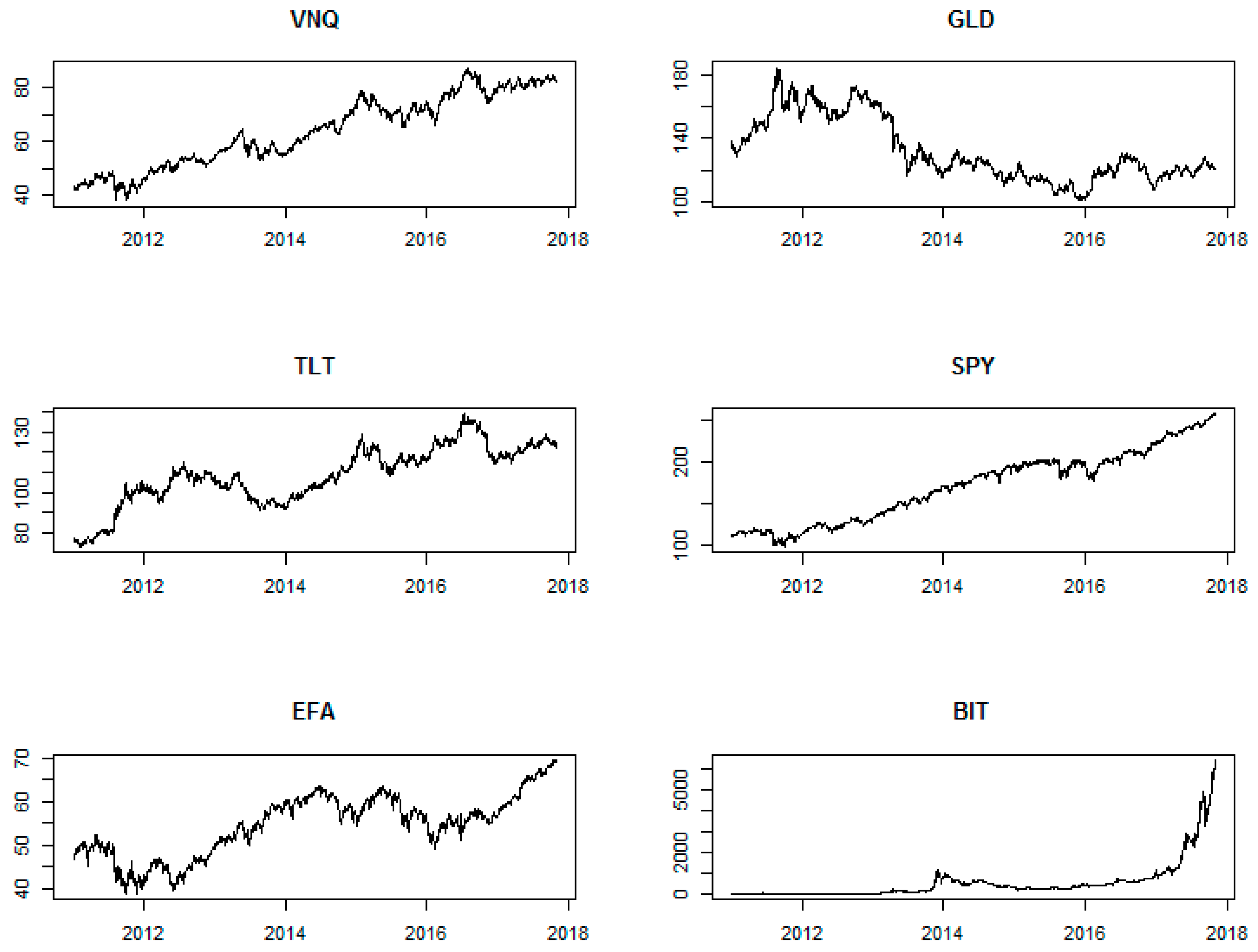
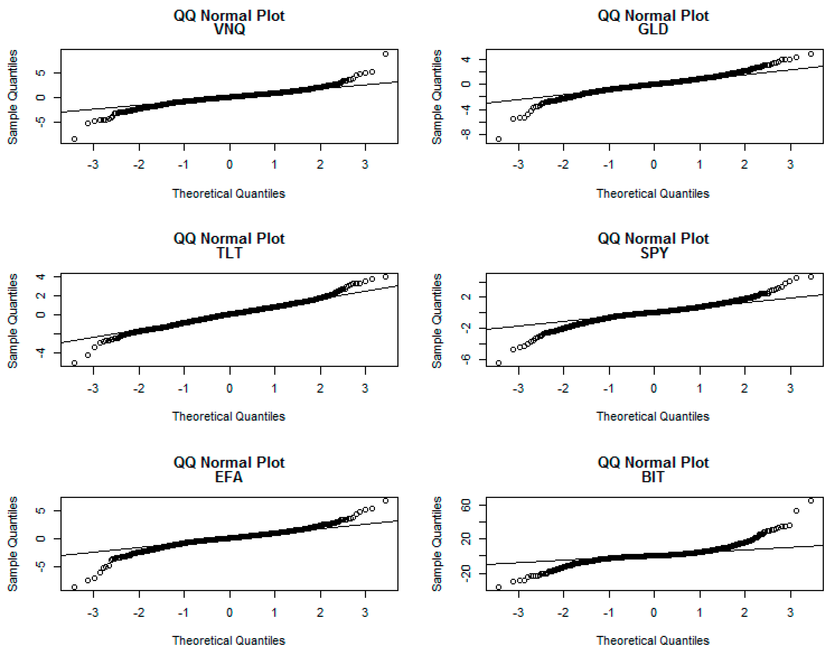
4. Data
5. Results
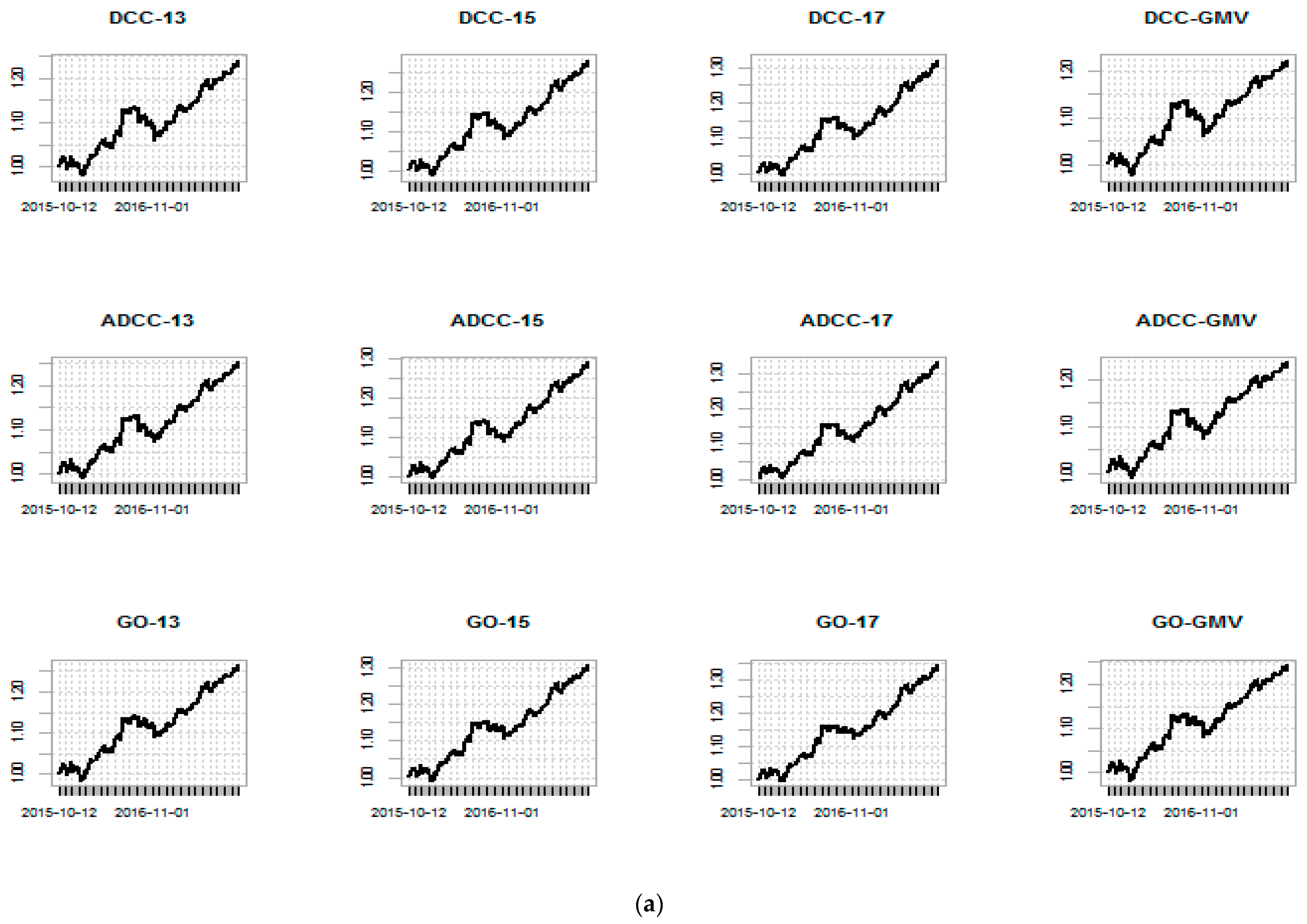
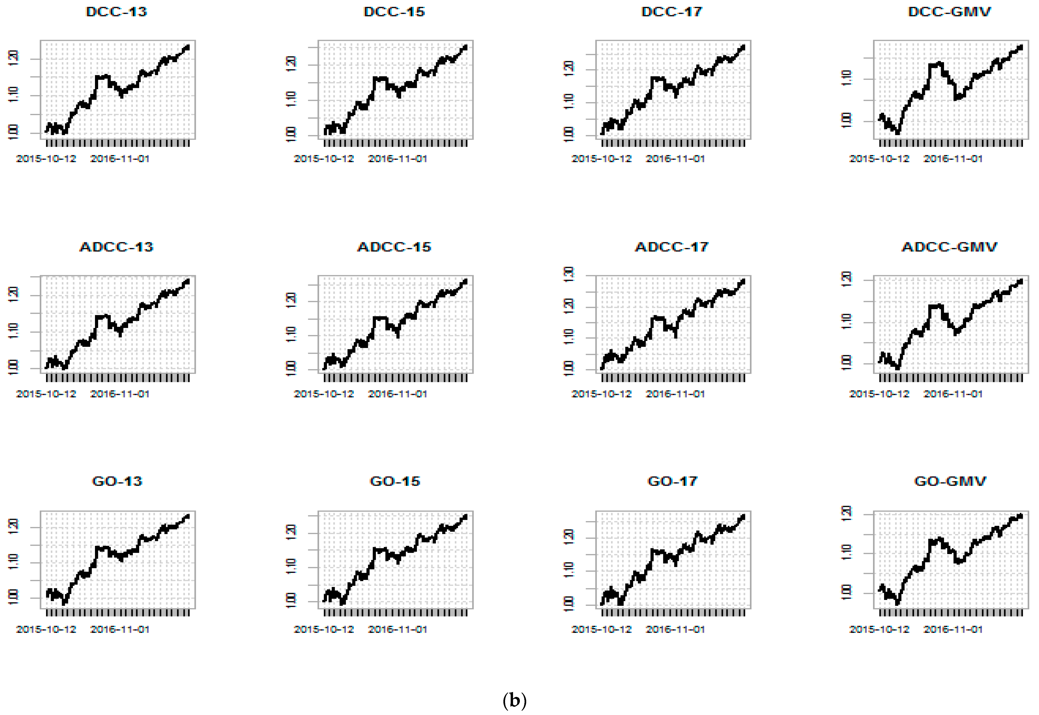
6. Robust Analysis: Long Only Portfolios
7. Conclusions and Implications
Author Contributions
Funding
Acknowledgments
Conflicts of Interest
References
- Aielli, Gian Piero. 2013. Dynamic Conditional Correlation: On Properties and Estimation. Journal of Business & Economic Statistics 31: 282–99. [Google Scholar] [CrossRef]
- Alexander, Carol. 2001. Market Models: A Guide to Financial Data Analysis. Chichester: John Wiley & Sons. [Google Scholar]
- Baur, Dirk G., and Brian M. Lucey. 2010. Is Gold a Hedge or a Safe Haven? An Analysis of Stocks, Bonds and Gold. Financial Review 45: 217–29. [Google Scholar] [CrossRef]
- Baur, Dirk G., and Thomas K. McDermott. 2010. Is Gold a Safe Haven? International Evidence. Journal of Banking & Finance 34: 1886–98. [Google Scholar] [CrossRef]
- Beckmann, Joscha, Theo Berger, and Robert Czudaj. 2015. Does Gold Act as a Hedge or a Safe Haven for Stocks? A Smooth Transition Approach. Economic Modelling 48: 16–24. [Google Scholar] [CrossRef]
- Böhme, Rainer, Nicolas Christin, Benjamin Edelman, and Tyler Moore. 2015. Bitcoin: Economics, Technology, and Governance. Journal of Economic Perspectives 29: 213–38. [Google Scholar] [CrossRef]
- Boswijk, H. Peter, and Roy van der Weide. 2006. Wake Me up before You GO-GARCH. 2006/3. Amsterdam School of Economics. Available online: http://dare.uva.nl/record/390623%5Cnpapers2://publication/uuid/A8691D04-AD04-42B6-8F98-34FD4CA86521 (accessed on 15 March 2018).
- Boswijk, H. Peter, and Roy van der Weide. 2011. Method of Moments Estimation of GO-GARCH Models. Journal of Econometrics 163: 118–26. [Google Scholar] [CrossRef]
- Bouri, Elie, Peter Molnár, Georges Azzi, David Roubaud, and Lars Ivar Hagfors. 2017. On the Hedge and Safe Haven Properties of Bitcoin: Is It Really More than a Diversifier? Finance Research Letters 20: 192–98. [Google Scholar] [CrossRef]
- Broda, Simon A., and Marc S. Paolella. 2009. CHICAGO: A Fast and Accurate Method for Portfolio Risk Calculation. Journal of Financial Econometrics 7: 412–36. [Google Scholar] [CrossRef]
- Canadian Federation of Independent Business. 2018. Regular vs. Premium Credit Card Rate Chart for Small Business. Toronto: CFIB. [Google Scholar]
- Caporin, Massimiliano, and Michael McAleer. 2013. Ten Things You Should Know about the Dynamic Conditional Correlation Representation. Econometrics 1: 115–26. [Google Scholar] [CrossRef]
- Cappiello, Lorenzo, Robert F. Engle, and Kevin Sheppard. 2006. Asymmetric Dynamics in the Correlations of Global Equity and Bond Returns. Journal of Financial Econometrics 4: 537–72. [Google Scholar] [CrossRef]
- Ciaian, Pavel, Miroslava Rajcaniova, and D’Artis Kancs. 2016. The Economics of BitCoin Price Formation. Applied Economics 48: 1799–815. [Google Scholar] [CrossRef]
- Ciner, Cetin, Constantin Gurdgiev, and Brian M. Lucey. 2013. Hedges and Safe Havens: An Examination of Stocks, Bonds, Gold, Oil and Exchange Rates. International Review of Financial Analysis 29: 202–11. [Google Scholar] [CrossRef]
- DeMiguel, Victor, Lorenzo Garlappi, Francisco J. Nogales, and Raman Uppal. 2009. A Generalized Approach to Portfolio Optimization: Improving Performance by Constraining Portfolio Norms. Management Science 55: 798–812. [Google Scholar] [CrossRef]
- Dyhrberg, Anne Haubo. 2016a. Bitcoin, Gold and the Dollar—A GARCH Volatility Analysis. Finance Research Letters 16: 85–92. [Google Scholar] [CrossRef]
- Dyhrberg, Anne Haubo. 2016b. Hedging Capabilities of Bitcoin. Is It the Virtual Gold? Finance Research Letters 16: 139–44. [Google Scholar] [CrossRef]
- Eichengreen, Barry. 1992. Golden Fetters: The Gold Standard and the Great Depression, 1919–1939. New York: Oxford University Press. [Google Scholar]
- Elton, Edwin J., and Martin J. Gruber. 1997. Modern Portfolio Theory, 1950 to Date. Journal of Banking and Finance 21: 1743–59. [Google Scholar] [CrossRef]
- Engle, Robert F. 2002. Dynamic Conditional Correlation: A simple class of multivariate generalized autoregressive conditional heteroskedasticity models. Journal of Business & Economic Statistics 20: 339–50. [Google Scholar] [CrossRef]
- Feibel, Bruce J. 2003. Investment Performance Measurement. Hoboken: John Wiley & Sons. [Google Scholar]
- Fleming, Jeff, Chris Kirby, and Barbara Ostdiek. 2001. The Economic Value of Volatility Timing. The Journal of Finance 56: 329–52. [Google Scholar] [CrossRef]
- Fry, John, and Eng-Tuck Cheah. 2016. Negative Bubbles and Shocks in Cryptocurrency Markets. International Review of Financial Analysis 47: 343–52. [Google Scholar] [CrossRef]
- Ghalanos, Alexios. 2015. Rmgarch: Multivariate GARCH Models. R Package Version 1.2-8. Available online: https://cran.r-project.org/web/packages/rmgarch/index.html (accessed on 15 March 2018).
- Glaser, Florian, Kai Zimmerman, Martin Haferkorn, Moritz Christian Weber, and Michael Siering. 2014. Bitcoin—Asset or Currency? Revealing Users’ Hidden Intentions. Paper presented at Twenty Second European Conference on Information Systems, Tel Aviv, Israel, June 9–14; pp. 1–14. [Google Scholar] [CrossRef]
- Glosten, Lawrence R., Ravi Jagannathan, and David E. Runkle. 1993. On the Relation between the Expected Value and the Volatility of the Nominal Excess Return on Stocks. The Journal of Finance 48: 1779–801. [Google Scholar] [CrossRef]
- Guesmi, Khaled, Samir Saadi, Ilyes Abid, and Zied Ftiti. 2018. Portfolio Diversification with Virtual Currency: Evidence from Bitcoin. International Review of Financial Analysis. [Google Scholar] [CrossRef]
- Hendrickson, Joshua R., Thomas L. Hogan, and William J. Luther. 2016. The Political Economy of Bitcoin. Economic Inquiry 54: 925–39. [Google Scholar] [CrossRef]
- Hillier, David, Paul Draper, and Robert Faff. 2006. Do Precious Metals Shine? An Investment Perspective. Financial Analysts Journal 62: 98–106. [Google Scholar] [CrossRef]
- Hopkins, Jamie. 2017. Bitcoin Might Be A ‘Bubble’ But Digital Currencies Are Not. Forbes, November 29. [Google Scholar]
- Jaffe, Jeffrey F. 1989. Gold and Gold Stocks as Investments for Institutional Portfolios. Financial Analysts Journal 45: 53–59. [Google Scholar] [CrossRef]
- Kim, Thomas. 2017. On the Transaction Cost of Bitcoin. Finance Research Letters 23: 300–5. [Google Scholar] [CrossRef]
- Kiviat, Trevor I. 2015. Beyond Bitcoin: Issues in Regulating Blockchain Transactions. Duke Law Journal 65: 569–608. [Google Scholar] [CrossRef]
- Ledoit, Oliver, and Michael Wolf. 2008. Robust Performance Hypothesis Testing with the Sharpe Ratio. Journal of Empirical Finance 15: 850–59. [Google Scholar] [CrossRef]
- Lo, Stephanie, and J. Christina Wang. 2014. Bitcoin as Money? Federal Reserve Bank of Boston 14: 1–28. [Google Scholar]
- McNutt, Patrick. 2002. The Economics of Public Choice II. Cheltenham: Edward Elgar Publishing. [Google Scholar]
- Michaud, By Richard, Robert Michaud, and Katharine Pulvermacher. 2006. Gold as a Strategic Asset. London: World Gold Council. [Google Scholar]
- Nakamoto, Satoshi. 2008. Bitcoin: A Peer-to-Peer Electronic Cash System. Available online: https://bitcoin.org/en/bitcoin-paper (accessed on 15 March 2018).
- Popper, Nathaniel. 2015a. Can Bitcoin Conquer Argentina? The New York Times, April 29. [Google Scholar]
- Popper, Nathaniel. 2015b. Digital Gold: Bitcoin and the Inside Story of Misfits and Millionaires Trying to Reinvent Money. New York: HarperCollins. [Google Scholar]
- R Core Team. 2015. R: A Language and Environment for Statistical Computing. R Foundation for Statistical Computing, Vienna, Austria. Available online: http://www.r-project.org/ (accessed on 15 March 2018).
- Reboredo, Juan C. 2013a. Is Gold a Hedge or Safe Haven against Oil Price Movements? Resources Policy 38: 130–37. [Google Scholar] [CrossRef]
- Reboredo, Juan C. 2013b. Is Gold a Safe Haven or a Hedge for the US Dollar? Implications for Risk Management. Journal of Banking & Finance 37: 2665–76. [Google Scholar] [CrossRef]
- Van Der Weide, Roy. 2002. GO-GARCH: A Multivariate Generalized Orthogonal GARCH Model. Journal of Applied Econometrics 17: 549–64. [Google Scholar] [CrossRef]
- Zhang, Kun, and Laiwan Chan. 2009. Efficient Factor GARCH Models and Factor-DCC Models. Quantitative Finance 9: 71–91. [Google Scholar] [CrossRef]
- Zhu, Yechen, David Dickinson, and Jianjun Li. 2017. Analysis on the Influence Factors of Bitcoin’s Price Based on VEC Model. Financial Innovation 3: 3. [Google Scholar] [CrossRef]
- Zohar, Aviv. 2015. Bitcoin. Communications of the ACM 58: 104–13. [Google Scholar] [CrossRef]
| 1 | Daily data are available at https://blockchain.info/charts. By convention, we use Bitcoin with a capital “B” to denote the Bitcoin network and “bitcoin” with a small “b” to denote the unit of account. |
| 2 | |
| 3 | The rotation matrix U needs to be estimated. For all but a few factors, maximum likelihood is not feasible. For a larger number of factors, alternative estimation methods must be used. ICA is a fast statistical technique for estimating hidden factors in relation to observable data. |
| 4 | Bitcoin price data was from 18 July 2010, but there was not much price variability over the first few months. |
| 5 | Summary statistics are computed using continuously compounded daily returns. Portfolio weights are estimated using discrete returns because discrete returns are additive across assets. The resulting portfolio returns are then converted to continuous returns for the calculation of portfolio summary statistics. |
| 6 | GARCH models are estimated using 1200 observations, and 519 one step forecasts are generated using rolling window estimation. The estimation window of 1200 observations is chosen based on a Monte Carlo comparison of RMSE. GARCH models are refitted every 60 observations. The portfolio results are robust to refits between 40 and 120 observations. |


| VNQ | GLD | TLT | SPY | EFA | BIT | |
|---|---|---|---|---|---|---|
| median | 0.083 | 0.024 | 0.076 | 0.061 | 0.052 | 0.247 |
| mean | 0.037 | −0.008 | 0.028 | 0.049 | 0.022 | 0.582 |
| SE.mean | 0.026 | 0.025 | 0.022 | 0.022 | 0.028 | 0.154 |
| CI.mean.0.95 | 0.052 | 0.050 | 0.042 | 0.042 | 0.054 | 0.301 |
| var | 1.193 | 1.100 | 0.799 | 0.805 | 1.316 | 40.537 |
| std.dev | 1.092 | 1.049 | 0.894 | 0.897 | 1.147 | 6.367 |
| coef.var | 29.151 | −134.32 | 32.012 | 18.296 | 53.190 | 10.934 |
| skewness | −0.364 | −0.610 | −0.121 | −0.572 | −0.778 | 0.148 |
| skew.2SE | −3.080 | −5.165 | −1.023 | −4.843 | −6.591 | 1.251 |
| kurtosis | 7.349 | 5.915 | 1.696 | 5.182 | 6.711 | 9.633 |
| kurt.2SE | 31.142 | 25.066 | 7.188 | 21.961 | 28.439 | 40.822 |
| normtest.W | 0.934 | 0.948 | 0.986 | 0.938 | 0.930 | 0.843 |
| normtest.p | 0.000 | 0.000 | 0.000 | 0.000 | 0.000 | 0.000 |
| VNQ | GLD | TLT | SPY | EFA | BIT | |
|---|---|---|---|---|---|---|
| VNQ | 1 | 0.07 * | −0.19 * | 0.73 * | 0.66 * | 0.07 * |
| GLD | 0.07 * | 1 | 0.2 * | −0.03 | 0.06 * | 0.02 |
| TLT | −0.19 * | 0.2 * | 1 | −0.5 * | −0.47 * | −0.02 |
| SPY | 0.73 * | −0.03 | −0.5 * | 1 | 0.88 * | 0.04 |
| EFA | 0.66 * | 0.06 * | −0.47 * | 0.88 * | 1 | 0.03 |
| BIT | 0.07 * | 0.02 | −0.02 | 0.04 | 0.03 | 1 |
| BIT | Mean | Sd | ||||||||
| VNQ | TLT | SPY | EFA | BIT | VNQ | TLT | SPY | EFA | BIT | |
| DCC-13 | −0.073 | 0.457 | 0.602 | −0.003 | 0.017 | 0.067 | 0.074 | 0.204 | 0.119 | 0.009 |
| DCC-15 | −0.073 | 0.441 | 0.653 | −0.050 | 0.028 | 0.068 | 0.079 | 0.224 | 0.133 | 0.010 |
| DCC-17 | −0.072 | 0.425 | 0.704 | −0.096 | 0.039 | 0.069 | 0.084 | 0.248 | 0.152 | 0.011 |
| DCC-GMV | −0.071 | 0.464 | 0.570 | 0.022 | 0.015 | 0.066 | 0.071 | 0.192 | 0.114 | 0.012 |
| ADCC-13 | −0.061 | 0.439 | 0.629 | −0.022 | 0.015 | 0.084 | 0.081 | 0.238 | 0.132 | 0.010 |
| ADCC-15 | −0.061 | 0.423 | 0.680 | −0.068 | 0.026 | 0.086 | 0.085 | 0.255 | 0.145 | 0.011 |
| ADCC-17 | −0.060 | 0.407 | 0.731 | −0.115 | 0.037 | 0.088 | 0.090 | 0.277 | 0.162 | 0.012 |
| ADCC-GMV | −0.059 | 0.446 | 0.595 | 0.006 | 0.012 | 0.084 | 0.081 | 0.235 | 0.134 | 0.012 |
| GO-13 | −0.126 | 0.483 | 0.654 | −0.028 | 0.017 | 0.087 | 0.055 | 0.122 | 0.064 | 0.007 |
| GO-15 | −0.127 | 0.468 | 0.702 | −0.072 | 0.028 | 0.086 | 0.063 | 0.141 | 0.087 | 0.008 |
| GO-17 | −0.128 | 0.453 | 0.751 | −0.116 | 0.040 | 0.087 | 0.072 | 0.167 | 0.113 | 0.010 |
| GO-GMV | −0.124 | 0.495 | 0.606 | 0.011 | 0.012 | 0.087 | 0.048 | 0.120 | 0.048 | 0.013 |
| GOLD | Mean | Sd | ||||||||
| VNQ | GLD | TLT | SPY | EFA | VNQ | GLD | TLT | SPY | EFA | |
| DCC−13 | −0.058 | −0.021 | 0.432 | 0.890 | −0.244 | 0.089 | 0.066 | 0.100 | 0.187 | 0.078 |
| DCC−15 | −0.047 | −0.089 | 0.447 | 1.049 | −0.360 | 0.103 | 0.081 | 0.116 | 0.208 | 0.088 |
| DCC−17 | −0.036 | −0.157 | 0.461 | 1.208 | −0.476 | 0.119 | 0.097 | 0.132 | 0.231 | 0.105 |
| DCC−GMV | −0.074 | 0.123 | 0.393 | 0.580 | −0.021 | 0.065 | 0.044 | 0.063 | 0.192 | 0.105 |
| ADCC−13 | −0.045 | −0.024 | 0.422 | 0.875 | −0.228 | 0.107 | 0.082 | 0.120 | 0.214 | 0.091 |
| ADCC−15 | −0.033 | −0.093 | 0.435 | 1.033 | −0.343 | 0.123 | 0.099 | 0.139 | 0.245 | 0.107 |
| ADCC−17 | −0.020 | −0.161 | 0.449 | 1.190 | −0.458 | 0.141 | 0.116 | 0.158 | 0.277 | 0.129 |
| ADCC−GMV | −0.064 | 0.115 | 0.381 | 0.597 | −0.030 | 0.073 | 0.047 | 0.068 | 0.228 | 0.120 |
| GO−13 | −0.087 | −0.004 | 0.436 | 0.948 | −0.293 | 0.075 | 0.044 | 0.058 | 0.177 | 0.066 |
| GO−15 | −0.076 | −0.076 | 0.456 | 1.104 | −0.408 | 0.082 | 0.055 | 0.063 | 0.191 | 0.072 |
| GO−17 | −0.065 | −0.149 | 0.476 | 1.260 | −0.523 | 0.092 | 0.067 | 0.071 | 0.207 | 0.081 |
| GO−GMV | −0.103 | 0.168 | 0.383 | 0.591 | −0.038 | 0.078 | 0.052 | 0.070 | 0.118 | 0.049 |
| Bitcoin Portfolio | ||||||||||||
| DCC-13 | DCC-15 | DCC-17 | DCC-GMV | ADCC-13 | ADCC-15 | ADCC-17 | ADCC-GMV | GO-13 | GO-15 | GO-17 | GO-GMV | |
| Mean | 11.737 | 13.684 | 15.623 | 10.899 | 12.277 | 14.244 | 16.204 | 11.483 | 12.954 | 14.934 | 16.906 | 11.881 |
| Sd | 6.340 | 6.462 | 6.694 | 6.325 | 6.139 | 6.261 | 6.497 | 6.115 | 6.463 | 6.589 | 6.830 | 6.427 |
| Sharp | 1.823 | 2.089 | 2.307 | 1.694 | 1.970 | 2.246 | 2.466 | 1.848 | 1.976 | 2.239 | 2.449 | 1.820 |
| Sharpe VaR | 1.194 | 1.384 | 1.542 | 1.104 | 1.298 | 1.497 | 1.659 | 1.212 | 1.303 | 1.492 | 1.646 | 1.192 |
| Sharpe ES | 0.937 | 1.084 | 1.205 | 0.868 | 1.018 | 1.171 | 1.295 | 0.951 | 1.021 | 1.167 | 1.285 | 0.936 |
| Sortino | 0.170 | 0.198 | 0.222 | 0.156 | 0.189 | 0.218 | 0.243 | 0.175 | 0.190 | 0.218 | 0.241 | 0.173 |
| Omega | 0.365 | 0.427 | 0.475 | 0.338 | 0.400 | 0.464 | 0.514 | 0.372 | 0.393 | 0.452 | 0.499 | 0.359 |
| Information | 1.849 | 2.153 | 2.411 | 1.705 | 2.010 | 2.328 | 2.591 | 1.872 | 2.024 | 2.329 | 2.582 | 1.847 |
| Drawdown | 0.074 | 0.069 | 0.064 | 0.077 | 0.062 | 0.057 | 0.051 | 0.065 | 0.055 | 0.050 | 0.044 | 0.054 |
| Gold Portfolio | ||||||||||||
| DCC-13 | DCC-15 | DCC-17 | DCC-GMV | ADCC-13 | ADCC-15 | ADCC-17 | ADCC-GMV | GO-13 | GO-15 | GO-17 | GO-GMV | |
| Mean | 11.589 | 12.594 | 13.578 | 8.774 | 11.827 | 12.941 | 14.035 | 9.888 | 11.565 | 12.368 | 13.151 | 9.644 |
| Sd | 6.843 | 7.610 | 8.554 | 6.098 | 6.613 | 7.377 | 8.324 | 5.907 | 6.813 | 7.561 | 8.478 | 6.112 |
| Sharp | 1.667 | 1.631 | 1.566 | 1.409 | 1.761 | 1.729 | 1.664 | 1.643 | 1.671 | 1.612 | 1.530 | 1.548 |
| Sharpe VaR | 1.085 | 1.060 | 1.015 | 0.907 | 1.150 | 1.128 | 1.083 | 1.068 | 1.087 | 1.046 | 0.990 | 1.003 |
| Sharpe ES | 0.853 | 0.834 | 0.799 | 0.715 | 0.904 | 0.887 | 0.851 | 0.840 | 0.855 | 0.823 | 0.779 | 0.789 |
| Sortino | 0.156 | 0.152 | 0.146 | 0.130 | 0.166 | 0.162 | 0.156 | 0.156 | 0.158 | 0.151 | 0.142 | 0.149 |
| Omega | 0.346 | 0.338 | 0.318 | 0.274 | 0.362 | 0.356 | 0.337 | 0.323 | 0.339 | 0.324 | 0.303 | 0.297 |
| Information | 1.683 | 1.653 | 1.592 | 1.387 | 1.784 | 1.762 | 1.701 | 1.641 | 1.686 | 1.631 | 1.549 | 1.540 |
| Drawdown | 0.063 | 0.058 | 0.063 | 0.086 | 0.059 | 0.062 | 0.069 | 0.073 | 0.046 | 0.050 | 0.054 | 0.065 |
| DCC-13 | DCC-15 | DCC-17 | DCC-GMV | ADCC-13 | ADCC-15 | ADCC-17 | ADCC-GMV | GO-13 | GO-15 | GO-17 | GO-GMV | |
|---|---|---|---|---|---|---|---|---|---|---|---|---|
| Diff | 0.010 | 0.028 | 0.046 | 0.018 | 0.013 | 0.032 | 0.050 | 0.013 | 0.019 | 0.039 | 0.057 | 0.017 |
| p value | 0.611 | 0.257 | 0.146 | 0.230 | 0.476 | 0.192 | 0.115 | 0.389 | 0.351 | 0.142 | 0.070 | 0.345 |
| DCC-13 | DCC-15 | DCC-17 | DCC-GMV | ADCC-13 | ADCC-15 | ADCC-17 | ADCC-GMV | GO-13 | GO-15 | GO-17 | GO-GMV | |
|---|---|---|---|---|---|---|---|---|---|---|---|---|
| γ = 1 | 14.873 | 109.067 | 204.591 | 212.566 | 45.007 | 130.366 | 217.066 | 159.585 | 139.024 | 256.772 | 375.691 | 223.790 |
| γ = 5 | 28.161 | 141.374 | 261.263 | 206.981 | 57.096 | 160.762 | 271.158 | 154.603 | 148.323 | 284.251 | 426.049 | 215.929 |
| γ = 10 | 44.840 | 181.937 | 332.429 | 199.976 | 72.271 | 198.929 | 339.095 | 148.353 | 159.995 | 318.748 | 489.280 | 206.067 |
| DCC-13 | DCC-15 | DCC-17 | DCC-GMV | ADCC-13 | ADCC-15 | ADCC-17 | ADCC-GMV | GO-13 | GO-15 | GO-17 | GO-GMV | |
|---|---|---|---|---|---|---|---|---|---|---|---|---|
| BIT | 0.125 | 0.136 | 0.148 | 0.129 | 0.129 | 0.140 | 0.153 | 0.133 | 0.078 | 0.093 | 0.109 | 0.074 |
| Gold | 0.128 | 0.148 | 0.172 | 0.129 | 0.136 | 0.157 | 0.182 | 0.133 | 0.063 | 0.073 | 0.085 | 0.065 |
| TC = $5 | ||||||||||||
| BIT | 1.576 | 1.708 | 1.870 | 1.623 | 1.620 | 1.759 | 1.931 | 1.673 | 0.979 | 1.169 | 1.378 | 0.927 |
| Gold | 1.618 | 1.870 | 2.163 | 1.624 | 1.716 | 1.977 | 2.288 | 1.678 | 0.788 | 0.916 | 1.069 | 0.821 |
| TC = $10 | ||||||||||||
| BIT | 3.151 | 3.417 | 3.741 | 3.247 | 3.239 | 3.518 | 3.862 | 3.347 | 1.959 | 2.338 | 2.756 | 1.854 |
| Gold | 3.236 | 3.741 | 4.326 | 3.247 | 3.432 | 3.954 | 4.576 | 3.355 | 1.576 | 1.832 | 2.138 | 1.641 |
| TC = $20 | ||||||||||||
| BIT | 6.303 | 6.833 | 7.481 | 6.493 | 6.479 | 7.035 | 7.725 | 6.693 | 3.917 | 4.676 | 5.511 | 3.707 |
| Gold | 6.472 | 7.481 | 8.652 | 6.495 | 6.864 | 7.908 | 9.151 | 6.710 | 3.152 | 3.663 | 4.276 | 3.282 |
| BIT | GLD | |||||
|---|---|---|---|---|---|---|
| DCC-GMV | ADCC-GMV | GO-GMV | DCC-GMV | ADCC-GMV | GO-GMV | |
| Mean | 10.557 | 10.475 | 11.088 | 8.316 | 8.778 | 8.785 |
| Sd | 6.405 | 6.231 | 6.440 | 6.191 | 6.056 | 6.146 |
| Sharp | 1.620 | 1.652 | 1.693 | 1.314 | 1.419 | 1.400 |
| SharpeVaR | 1.052 | 1.074 | 1.103 | 0.843 | 0.914 | 0.901 |
| SharpeES | 0.828 | 0.845 | 0.867 | 0.665 | 0.721 | 0.710 |
| Sortino | 0.146 | 0.152 | 0.156 | 0.119 | 0.131 | 0.131 |
| Omega | 0.324 | 0.329 | 0.337 | 0.257 | 0.277 | 0.269 |
| Information | 1.623 | 1.656 | 1.706 | 1.285 | 1.398 | 1.378 |
| Drawdown | 0.081 | 0.071 | 0.065 | 0.093 | 0.082 | 0.077 |
| DCC-GMV | ADCC-GMV | GO-GMV | |
|---|---|---|---|
| γ = 1 | 224.177 | 169.771 | 230.425 |
| γ = 5 | 218.885 | 165.505 | 223.109 |
| γ = 10 | 212.250 | 160.155 | 213.935 |
| DCC-GMV | ADCC-GMV | GO-GMV | |
|---|---|---|---|
| BIT | 0.088 | 0.086 | 0.037 |
| Gold | 0.081 | 0.084 | 0.033 |
| TC = $5 | |||
| BIT | 1.104 | 1.088 | 0.465 |
| Gold | 1.019 | 1.055 | 0.410 |
| TC = $10 | |||
| BIT | 2.208 | 2.177 | 0.930 |
| Gold | 2.037 | 2.111 | 0.819 |
| TC = $20 | |||
| BIT | 4.415 | 4.353 | 1.860 |
| Gold | 4.075 | 4.221 | 1.638 |
© 2018 by the authors. Licensee MDPI, Basel, Switzerland. This article is an open access article distributed under the terms and conditions of the Creative Commons Attribution (CC BY) license (http://creativecommons.org/licenses/by/4.0/).
Share and Cite
Henriques, I.; Sadorsky, P. Can Bitcoin Replace Gold in an Investment Portfolio? J. Risk Financial Manag. 2018, 11, 48. https://doi.org/10.3390/jrfm11030048
Henriques I, Sadorsky P. Can Bitcoin Replace Gold in an Investment Portfolio? Journal of Risk and Financial Management. 2018; 11(3):48. https://doi.org/10.3390/jrfm11030048
Chicago/Turabian StyleHenriques, Irene, and Perry Sadorsky. 2018. "Can Bitcoin Replace Gold in an Investment Portfolio?" Journal of Risk and Financial Management 11, no. 3: 48. https://doi.org/10.3390/jrfm11030048
APA StyleHenriques, I., & Sadorsky, P. (2018). Can Bitcoin Replace Gold in an Investment Portfolio? Journal of Risk and Financial Management, 11(3), 48. https://doi.org/10.3390/jrfm11030048