An Empirical Study on the Impact of Basel III Standards on Banks’ Default Risk: The Case of Luxembourg

Abstract

We study how the Basel III regulations, namely the Capital-to-Assets Ratio (CAR), the Net Stable Funding Ratio (NSFR) and the Liquidity Coverage Ratio (LCR), are likely to impact banks’ profitability (i.e., ROA), capital levels and default. We estimate historical series of the new Basel III regulations for a panel of Luxembourgish banks for a period covering 2003q2–2011q3. We econometrically investigate whether historical LCR and NSFR components, as well as CAR positions are able to explain the variation in a measure of a bank’s default risk (approximated by Z-score) and how these effects make their way through banks’ ROA and CAR. We find that the liquidity regulations induce a decrease in average probabilities of default. We find that the liquidity regulation focusing on maturity mismatches (i.e., NSFR) induces a decrease in average probabilities of default. Conversely, the impact on banks’ profitability is less clear-cut; what seems to matter is banks’ funding structure rather than the characteristics of the portfolio of assets. Additionally, we use a model of bank behavior to simulate the banks’ optimal adjustments of their balance sheets as if they had to adhere to the regulations starting in 2003q2. Then, we predict, using our preferred econometric model and based on the simulated data, the banks’ Z-score and ROA. The simulation exercise suggests that basically all banks would have seen a decrease in their default risk during a crisis episode if they had previously adhered to Basel III.

1. Introduction

In response to the global financial crisis of 2007–2009, the Basel Committee on Banking Supervision1 (BCBS) decided to strengthen bank soundness by introducing new regulations, collectively called Basel III (BCBS 2014; BCBS 2013; BCBS 2010a; BCBS 2010b; Angelini et al. 2011). Our contribution in this article is to analyze whether or not these new regulations are likely to lead to a banking sector that will be in a better position to absorb shocks and thereby be more resilient in future crises. We focus on the three standards that are currently under evaluation, namely the leverage ratio (defined as the Capital-to-Asset Ratio, CAR), the Liquidity Coverage Ratio (LCR) and the Net Stable Funding Ratio (NSFR). These regulations target different sources of risk and are likely to have sizeable impacts on banks’ balance sheets and profits. The CAR measures how far banks are able to absorb losses. The CAR constrains banks in their ability to leverage up their balance sheets and may be viewed as countercyclical in nature (BCBS 2010b), especially due to the procyclicality of leverage (see Adrian and Shin 2010, Giordana and Schumacher 2012). The LCR is essentially a measure of a bank’s exposure to short-run liquidity risk (BCBS 2013, p. 1), while the NSFR is a measure of maturity mismatch aimed at promoting more medium and long-term funding (BCBS 2010a, p. 25).

Our main objective is to analyze whether and how the Basel III regulations will impact banks’ default risk. With this aim, we rely on a measure of distance-to-default commonly known as the Z-score index (see DeNicolo 2001, DeNicolo et al. 2004), which assesses to what extent banks’ equity can cover losses. In order to provide a more precise picture, we also study how these regulations impact the components of the Z-score.2 We proceed in three steps.

Our first step is to calculate the LCR and the NSFR based on bank level data for a sample that covers the 50 largest banks in Luxembourg for the period 2003q2–2011q3. Due to the level of detail required to construct the LCR and NSFR, banks’ statistical reporting to the central bank is used for this purpose.3 The sample time span stops before the implementation of the Basel III regulations; therefore, the standards have not been targeted by banks. This allows for a better identification as we can consider the historical positions of estimated LCR, NSFR and capital-to-assets ratio as bank balance-sheet characteristics (or business model) unaffected by policy.

As a second step, we empirically investigate the impact of the LCR, the NSFR and the capital-to-asset ratio on banks’ profitability (measured by the Return-Over-Assets ratio, ROA), leverage ratio and Z-score. The econometric specification we propose allows identifying how the impacts of the new regulations on default risk are likely to be channeled through banks’ profits and leverage decisions. Through this, we intend to obtain a precise picture of the potential effects of the Basel III regulations and of how the Z-score will potentially evolve once banks adhere to the new standards.

In the final step, we aim at measuring the effect of compliance with Basel III on banks’ default risk. One problem is that banks would need to optimally trade off several regulations, and thereby, the final impact on default probabilities depends on how banks achieve the balance sheet adjustments needed for compliance. To account for these trade-offs and substitution effects among the different balance sheet components, we simulate a model of bank behavior where banks maximize their profits subject to their balance sheet constraint, as well as to the new Basel III regulations. Thus, for each bank and each period, we obtain simulated balance sheet data (e.g., simulated CAR, high-quality-liquid assets) from 2003q2 onwards. We then use our regression results to predict the Z-score and ROA based on our simulated data. Finally, we compare the observed and the simulated Z-score and ROA, which provides us with an understanding of whether or not we should expect lower probabilities of default and a less profitable banking sector due to Basel III.

The kind of exercise we implement suffers from the caveats related to potential instability of the statistical relationships identified using historical data. In particular, Goodhart’s law asserts “that any observed statistical regularity will tend to collapse once pressure is placed upon it for control purposes”.4 However, the level of granularity of the banks’ balance sheet data we use tends to restrain the validity of the critique for our case.

Our main results are as follows. In our econometric analysis, we find that the new regulations induce a statistically-significant decrease in banks’ probabilities of default. The disaggregated analysis on the components of the measure of distance-to-default allowed us to identify channels through which Basel III would mainly impact. We show that the impact on default risk would essentially be driven by the regulatory limits to the leverage ratio (i.e., inverse of CAR) and the components of the NSFR. Indeed, our findings point out that a higher NSFR relates to a higher level of bank capitalization for those banks that have a sufficient amount of stable funding, and it also relates to a higher return-on-assets. Finally, the econometric results indicate that the effect of the LCR on banks’ profitability goes through the level of net outflows (i.e., the denominator of LCR) and that a higher capital-to-asset ratio is associated with a lower return on assets. This suggests that better capitalized banks tend to have a more cautious investment profile and a lower return on equity given the level of total assets. As expected, we also find a positive relationship between CAR and ROA, suggesting that banks tend to increase their capital through retained earnings.

Based on the simulation outcome and on our preferred econometric models, we predict that, at the median, banks would have seen their probabilities of default decrease during a crisis episode if they had previously adhered to the regulations. This result is due to improvements in both banks’ profitability and capitalization. Thus, we conclude that the Basel III regulation will diminish bank default risk and thereby improve the resilience of the financial sector. As the new Basel III ratios will also be applied globally and given the soundness of the empirical strategy implemented, we would expect the results presented here to equally apply to other banking sectors.

While Basel III regulations have an explicit macro-prudential perspective, our approach is micro-oriented, as we focus on the impact on individual institutions. Nevertheless, our results have also implications on the mitigation of systemic risk beyond the time-related transmission channels targeted by the ratios analyzed in this study. As regards the structural dimension of systemic risk, the financial soundness of systemically-important banks plays a fundamental role. While there are alternative measures that can be used to identify systemically-important banks,5 it is also well-known that the size of bank’s balance sheet correlates strongly with these (Drehmann and Tarashev 2011; Moore and Zhou 2013).6 Our results imply that the Basel III ratios would mitigate systemic risk during a crisis episode. However, it should be clear that this result is not necessarily valid externally, and thus, it should be viewed as a first conclusion that warrants further analysis in other banking sectors.

There exist now several articles that study the impact of the Basel III regulations (see BCBS 2010; Slovik and Cournède 2011; Giordana and Schumacher 2013). Most large-scale studies have been undertaken by the BCBS itself. However, the main focus is on the shortfalls associated with the regulations, as well as on some potential impacts through dynamic general equilibrium models. We view our econometric approach as complementary to their analysis and our estimation of the predicted Z-score and banks’ profitability and capitalization, under compliance with Basel III (based on the simulated data), as the actual novelty. Our article is also related to the large literature on capital regulation and risk-taking (e.g., Lam and Chen 1985; Gennotte and Pyle 1991; Besanko and Kanatas 1996; Wagner 2007). These articles study, theoretically or empirically, the relationship between capital regulation, banks’ liquidity and their risk-taking. We contribute to this literature by our empirical assessment of the latest Basel III regulation. In addition, we complement existing results on the positive impact of bank soundness and information provision (e.g., Demirgüç-Kunt et al. 2008; Barth et al. 2004; Podpiera 2006). Finally, we contribute to the large literature on banks’ profitability (see Berger 1995; Goddard et al. 2004; Athanasoglou et al. 2008; Berger and Bouwman 2010, among others) by providing additional empirical evidence based on a comprehensive assessment of liquidity risk and on robust econometric estimations.

The article is organized as follows. Section 2 discusses the chosen measure of distance-to-default and, based on the empirical literature on banks’ profitability, the endogenous relationship between banks’ leverage and profits. Additionally, the Basel III standards are described. Section 3 presents the econometric specification and Section 4 the data used in the study. In Section 5, the results of the econometric study and of the simulation exercise are presented and analyzed. Finally, Section 6 concludes.

2. Basel III Regulations and the Probability of Default

2.1. Probability of Default, Leverage and Profitability of Banks

The economic and finance literature provides several measures of probability of default linked to credit risk (see, e.g., Merton 1974; Duffie and Singleton 2003; Campbell et al. 2008; Basurto and Espinoza 2011; Chan-Lau and Sy 2007, and for applications to Luxembourg, see Jin and Nadal de Simone 2011). In this study, we resort to the Z-score index as the measure of bank distance-to-default7, which has increasingly been used in the academic literature (see, e.g., DeNicolo 2001; DeNicolo et al. 2004; Berger et al. 2009; Wolff and Papanikolaou 2015; Maechler et al. 2007). The Z-score is a measure of distance-to-default that can be derived from balance sheet and profit and loss data without relying on market valuations.8 It is calculated as:

$${\mathrm{Z}-\mathrm{score}}_{it}=\frac{{\mathrm{E}}_{it}/{\mathrm{A}}_{it}+{\mathrm{ROA}}_{it}}{\mathrm{sd}\left({\mathrm{ROA}}_{it}\right)}.$$

(1)

where ${\mathrm{E}}_{it}$ is bank i’s Tier 1 capital at time t, ${\mathrm{A}}_{it}$ are its total assets, then ${\mathrm{E}}_{it}/{\mathrm{A}}_{it}$ is the Capital-Assets Ratio (CAR), ${\mathrm{ROA}}_{it}$ is the return on assets calculated as after tax profits divided by total assets and $\mathrm{sd}({\mathrm{ROA}}_{it})$ is the standard deviation of ${\mathrm{ROA}}_{it}$. It is a measure of insolvency risk insofar as the square of its inverse is the probability that losses exceed equity for normally-distributed returns.

The appeal of this indicator as a proxy for banks’ distance-to-default relies on the few assumptions that underlie this measure and on its transparency and conclusive link to banks’ fundamentals. However, some issues arise when coming to understand the impact of changes in its components. Looking at Equation (1), one would be inclined to conclude that banks with higher leverage (i.e., CAR${}^{-1}$) would be penalized by this index, since these banks have a smaller share of equity that could compensate for their losses. Similarly, one may expect that higher ${\mathrm{ROA}}_{it}$ leads to lower default risk and that the standard deviation on the return on assets, $\mathrm{sd}({\mathrm{ROA}}_{it})$, reduces the Z-score since it increases the probability that equity falls short of losses. However, opposite conclusions might be reached once the simultaneity of CAR and ROA is taken into account. In other words, the level of leverage affects the ROA and vice versa, modifying the relationship between the Z-score and its components. For example, if a bank improves its ROA by increasing its leverage, it is entirely possible that the increase in ROA brings this bank closer to default.

One would expect that a higher level of capital reduces the return on assets as it might signal that the bank is implementing a cautious investment strategy. Thus, other things equal, it reduces the risk on equity. However, a number of studies have found a positive relationship between capital and profits (Berger 1995; Goddard et al. 2004; Athanasoglou et al. 2008; Berger and Bouwman 2010), while others found a negative one (Goddard et al. 2004). This suggests a bi-directional causal relationship between capital (or leverage) and profitability. Indeed, using a Granger-causality test, Berger (1995) finds a positive association between CAR and Return-On-Equity (ROE) in both senses of the causal relationship. The arguments backing the negative relationship are consistent with the standard one period model of perfect capital markets with symmetric information between a bank and its investors. Though, as Berger (1995) suggests, relaxing the assumptions of this model may yield the opposite results. For example, an asset expansion that is fueled by attracting additional deposits (i.e., reduction in CAR) would reduce a bank’s profits if the deposit supply curve faced by the bank is upward slopping.

The empirical evidence on banks’ profitability suggests that a bank’s leverage and profits might be related or simultaneously determined. As a consequence, the endogeneity issue should be reflected in the choice of the econometric methodology in order to deal with the potential bias of the estimations. In particular, Instrumental Variable (IV) estimators should be employed. The empirical studies within this literature examine bank-specific, industry and macroeconomic determinants of profitability defined as ROA or Return-On-Equity (ROE). Among the macroeconomic factors considered are the inflation rate and the long-term interest rate (Molyneux and Thornton 1992; Bourke 1989), as well as GDP growth (Demirgüç-Kunt and Huizinga 1999), the unemployment rate and interest rate differentials (Bikker and Hu 2002). The industry-level determinants studied relate to measures of market concentration and industry size (Berger 1995; Smirlock 1985). Finally, among the subset of bank-specific determinants employed, one can find variables such as capital, size, efficiency, credit and liquidity risk indicators (Athanasoglou et al. 2008; Goddard et al. 2004; Goddard et al. 2004; Berger 1995; Demirgüç-Kunt and Huizinga 1999; Berger and Bouwman 2010). Besides the assessment of the potential impact of the new regulations on profitability, we contribute to this literature by considering more sophisticated indicators of liquidity risk. Indeed, liquidity risk measures the ability of generating enough inflows to meet the net cumulative cash outflow within a certain time period. We propose to take into account all of the dimensions of liquidity risk, namely the encumbrance and marketability of assets, the cash-flows and the maturity structure of a bank’s balance sheet. Thus, we include as regressors the components of the Basel III liquidity regulations, which we describe in the next section.

2.2. The Basel III Regulations

On the background of the global financial crisis of 2007–2009, the BCBS introduced several new regulations and supervisory tools for banks in order to improve their resilience to shocks. The new regulatory framework enhances the risk coverage and the consistency of the capital base, reduces the procyclicality, banks’ liquidity risk and their maturity mismatches (BCBS 2013; BCBS 2010a; BCBS 2010b). Among the set of regulations, we focus on three new standards, namely the Capital-to-Assets Ratio (CAR), the Liquidity Coverage Ratio (LCR) and the Net Stable Funding Ratio (NSFR).

The CAR is defined as Tier 1 capital divided by total assets. The current Basel III proposal demands banks to hold a CAR of 3% (see p. 64 in BCBS (2010b) and p. 1 in BCBS (2014)). It ensures that banks are able to cover a sufficient percentage of total assets with their own funds and constrains procyclicality by limiting the build up of leverage. In addition, given that it is a non-risk-based capital requirement, it will also contribute to the dampening of the procyclical behavior of banks by de-linking the level of total regulatory capital required from the evolution of risk perceptions.

The LCR is introduced to improve banks’ ability to cope with short-run liquidity needs and market liquidity risk.9 It is calculated as the ratio of the stock of High Quality Liquid Assets (HQLA) over the net cash outflows that are expected to arise during one month under an acute stress scenario. Once implemented, banks will be required to adjust their balance sheets such that this ratio is at least equal to one, meaning that the stock of HQLA covers the expected net outflows for one month. High quality liquid assets comprise those unencumbered assets that may be easily converted into cash without significant haircuts, for example highly rated government securities. Outflows comprise deposits and other funding sources that a bank might lose during a period of stress. These liabilities receive different haircuts depending on how stable they are expected to be during financial distress. Net Outflows (NO) then are calculated as outflows minus inflows, where only those inflows are included that are expected to be fully performing. Furthermore, inflows are restricted to 75% of outflows in order to assure that banks hold a certain minimum of liquid assets.

The Net Stable Funding Ratio (NSFR) is a measure of maturity mismatch risk aimed at promoting more medium-term and long-term funding of the assets of a bank. Thus, the NSFR tends to reduce the exposure to funding liquidity risk.10 It demands the amount of Available Stable Funding (ASF) to be greater than or equal to the amount of Required Stable Funding (RSF). The ASF consists of capital, liabilities with maturity greater than a year or those that are expected to be stable during a stress period. The RSF places more weight on those assets that are less liquid during stress periods and therefore require a more stable source of funding. Banks that fall short of the NSFR requirement will need to either increase their capital, or those liabilities that are not likely to be withdrawn during stressed periods, or to reduce their investments in less liquid assets.

3. Econometric Specification

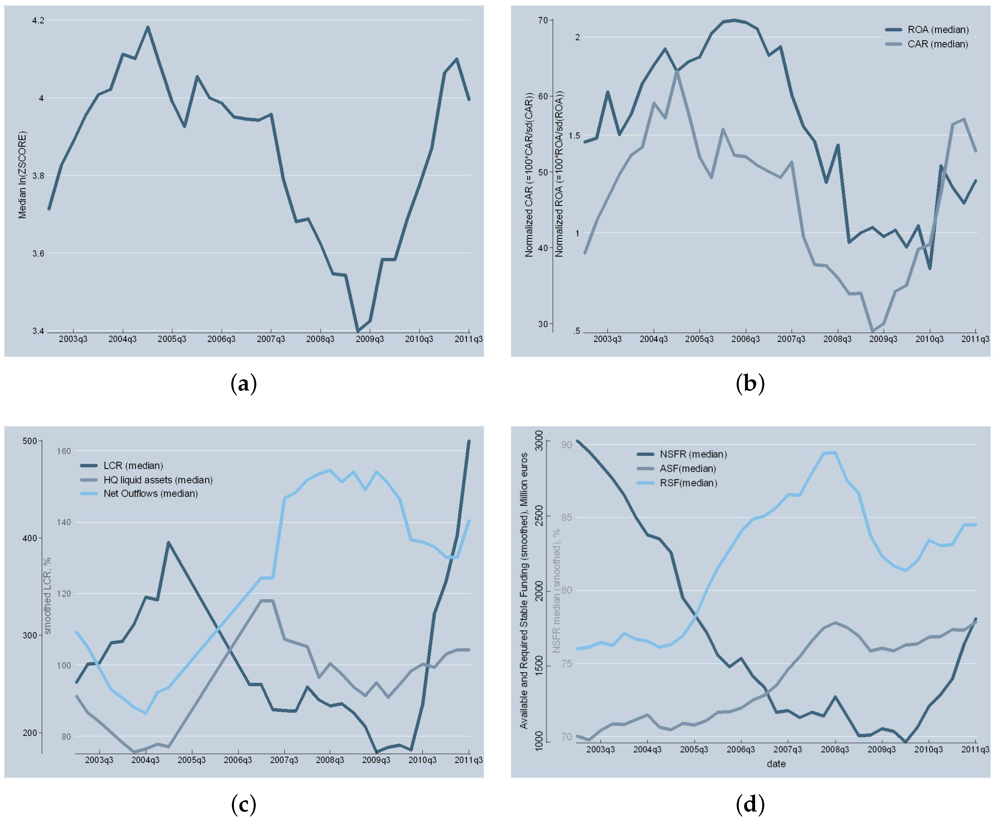
In this subsection, we describe the econometric model specification and explain the choice of the estimators. We start with the model specification for the main components of the Z-score, namely the capital-to-assets and return-on-assets ratios. Then, we describe the econometric specification for the Z-score. We normalize ROA and CAR by the standard deviation of ROA (i.e., ${\sigma }_{ROA}$) because this allows us to derive straightforwardly the Z-score model (Equation (4)) by substituting Equations (2) and (3) in definition (1). The interpretation of the econometric results should be done taking into account this transformation.

In terms of bank behavior, we are assuming that banks choose their level of leverage in order to improve future profitability. This means that leverage affects future profits. In addition, higher profits today would allow increasing the equity share through retained earnings. Thus, leverage is contemporaneously related to the return-on-assets. Therefore, we consider CAR as a predetermined regressor in the ROA model11 and the ROA series as endogenous in the CAR model.12

The return-on-assets is a commonly-used indicator of banks’ profitability, which measures the ability of the bank’s management to generate profits given the asset size. However, this variable might be a biased measure of profitability if the off-balance sheet activities represent an important share of a bank’s return. Hence, we include the ratio between the off-balance sheet commitments and total assets as a control variable. We specify a dynamic model for ROA by including one lag of the dependent variable as a regressor. This allows us to evaluate the degree of profit persistence. Similar to previous empirical studies, we consider, as determinants of banks’ profitability, several bank-specific variables, as well as macroeconomic indicators. Hence, we include a comprehensive set of bank-specific characteristics, such as the capital-to-assets ratio (i.e., the inverse of leverage), the balance sheet size (measured by total assets) and indicators of liquidity risk and efficiency. Most importantly, we introduce our calculations of the new liquidity regulations (i.e., the components of the LCR and NSFR) as liquidity risk proxies. Furthermore, we look at the efficiency of banks by means of the ratio of gross income over administrative and labor expenses. Finally, we account for the impact of macroeconomic and funding conditions on bank profits by considering the GDP growth rate, the GDP gap and the change in the short-term interest rate (i.e., Euribor three months) as regressors, though only the later variable is retained in the final specification.13

The capital-to-assets ratio, the second component of the Z-score that we study, is an indicator of the bank risk profile. As is the case for the ROA model, we include one lag of the dependent variable as a regressor, and we consider bank-specific and macroeconomic indicators as determinants of CAR. As previously discussed, we include the contemporaneous level of ROA. As indicators of liquidity risk, we also consider the components of the Basel III liquidity ratios (over total assets), namely the ratio of high-quality liquid assets, the net-outflows ratio, as well as the amounts of available and required stable funding. Finally, we include the change in the short-term interest rate, as well as crises and seasonal dummies.

The ROA and CAR specifications are given in Equations (2) and (3).

$$\begin{array}{ccc}\hfill {\left(\frac{\mathrm{ROA}}{{\sigma }_{\mathrm{ROA}}}\right)}_{it}& =& {\alpha }_{1,0}+{\alpha }_{1,1}{\left(\frac{\mathrm{ROA}}{{\sigma }_{\mathrm{ROA}}}\right)}_{it-1}+{\alpha }_{1,2}{\left(\frac{\mathrm{CAR}}{{\sigma }_{\mathrm{ROA}}}\right)}_{it-1}\hfill \\ \mathrm{(2)}& & & +{\alpha }_{1,3}{\mathrm{HQLAR}}_{it-1}+{\alpha }_{1,4}{\mathrm{NOR}}_{it-1}+{\alpha }_{1,5}{\mathrm{ASFR}}_{it-1}+{\alpha }_{1,6}{\mathrm{RSFR}}_{it-1}\hfill & & +{\alpha }_{1,7}ln({\mathrm{TA}}_{it-1})+{\alpha }_{1,8}{\mathrm{OBSR}}_{it-1}+{\alpha }_{1,9}{\mathrm{EFF}}_{it-1}+{\alpha }_{1,10}\Delta {\mathrm{IR}}_t\hfill \\ & & +{\alpha }_{1,11}{C}_{lt}+{\alpha }_{1,12}{C}_{st}+\sum _{q=Q2}^{Q4}{\alpha }_{1,q}{d}_q+{ϵ}_{1,it},\hfill \end{array}$$

$$\begin{array}{ccc}\hfill {\left(\frac{\mathrm{CAR}}{{\sigma }_{\mathrm{ROA}}}\right)}_{it}& =& {\alpha }_{2,0}+{\alpha }_{2,1}{\left(\frac{\mathrm{CAR}}{{\sigma }_{\mathrm{ROA}}}\right)}_{it-1}+{\alpha }_{2,2}{\left(\frac{\mathrm{ROA}}{{\sigma }_{\mathrm{ROA}}}\right)}_{it}\hfill \\ \mathrm{(3)}& & & +{\alpha }_{2,3}{\mathrm{HQLAR}}_{it-1}+{\alpha }_{2,4}{\mathrm{NOR}}_{it-1}+{\alpha }_{2,5}{\mathrm{ASFR}}_{it-1}+{\alpha }_{2,6}{\mathrm{RSFR}}_{it-1}\hfill & & +{\alpha }_{2,7}ln({\mathrm{TA}}_{it-1})+{\alpha }_{2,9}{\mathrm{EFF}}_{it-1}+{\alpha }_{2,10}\Delta {\mathrm{IR}}_t\hfill \\ & & +{\alpha }_{2,11}{C}_{lt}+{\alpha }_{2,12}{C}_{st}+\sum _{q=Q2}^{Q4}{\alpha }_{2,q}{d}_q+{ϵ}_{2,it},\hfill \end{array}$$

$$\begin{array}{ccc}\hfill {\mathrm{Z}-\mathrm{score}}_{it}& =& {\beta }_0+{\beta }_1{\left(\frac{\mathrm{ROA}}{{\sigma }_{\mathrm{ROA}}}\right)}_{it-1}+{\beta }_2{\left(\frac{\mathrm{CAR}}{{\sigma }_{\mathrm{ROA}}}\right)}_{it-1}\hfill \\ \mathrm{(4)}& & & +{\beta }_3{\mathrm{HQLAR}}_{it-1}+{\beta }_4{\mathrm{NOR}}_{it-1}+{\beta }_5{\mathrm{ASFR}}_{it-1}+{\beta }_6{\mathrm{RSFR}}_{it-1}\hfill & & +{\beta }_{7}ln({\mathrm{TA}}_{it-1})+{\beta }_8{\mathrm{OBSR}}_{it-1}+{\beta }_9{\mathrm{EFF}}_{it-1}+{\beta }_{10}\Delta {\mathrm{IR}}_t\hfill \\ & & +{\beta }_{11}{C}_{lt}+{\beta }_{12}{C}_{st}+\sum _{q=Q2}^{Q4}{\beta }_q{d}_q+{ϵ}_{zs,it}.\hfill \end{array}$$

where, as defined in Section 2.2, the HQLAR, NOR, ASFR and RSFR are, respectively, the stock of high-quality liquid assets to total assets ratio, the amount of net-outflows total assets ratio and the level of available and required stable funding over total assets; OBSR is the off-balance sheet commitments to total assets ratio; EFF is an indicator of a bank’s efficiency; $\Delta$IR${}_t$ is the change in the short-term interest rate; C${}_{lt}$ and C${}_{st}$ are binary variables indicating, respectively, the 2007–2009 liquidity crisis and the European sovereign debt crisis; $d_q$ are seasonal dummies (i.e., one per quarter); and ${ϵ}_{j,it}={\mu }_{j,i}+{\nu }_{j,it},j=1,2,zs$ represents the error term, which encompasses individual fixed effects (i.e., ${\mu }_{j,i}$). The abbreviations section below provides a precise definition of each variable.

Given definition (1), the coefficients ${\beta }_j$ in Equation (4) are non-linear combinations of the coefficients $\alpha$’s in Equations (2) and (3).14 The estimation of the $\alpha$ and $\beta$ parameters can be either done by running estimations for each equation separately or for the system of equations formed by the triplet. In order to deal with the bias introduced through the dynamic specification15 in Equations (2)–(4),16, and through the assumed pre-determined relationship between ROA and CAR, we adopt an equation-by-equation estimation strategy and resort to a type of Generalized Method of Moments (GMM) instrument variables estimator known as system-GMM (Arellano and Bond 1991; Arellano and Bover 1995; Blundell and Bond 1998). In addition to the traditional specification tests (i.e., non-autocorrelation of the errors, exogeneity of the matrix of instruments), we verify that the coefficient of the lagged dependent variable estimated by the system-GMM estimator falls in the interval given by the coefficient estimated by the ordinary least squares and within estimators. Moreover, in order to keep the instrument exogeneity tests reliable, we systematically check that the number of instruments does not exceed the number of groups. Finally, aiming at dealing with potential heteroscedasticity and inter-group multicollinearity and to perform sound inferences, we recur to two-step robust standard errors with Windmeijer’s (Windmeijer 2005) finite sample correction.

However, a system-wide estimation strategy might increase the efficiency of estimates as it adds information from the potential relationship between equations of the system, though it does not deal with the dynamic panel bias and the potential simultaneity bias. In fact, given that the $\beta$ coefficients are non-linear combinations of coefficients $\alpha$ (Equations (2) and (3)), the efficiency improvement might be sizeable. Moreover, considering that we have a panel dataset with 35 periods, the dynamic-panel bias may be low (Judson and Owen 1999). In such a case, a seemingly unrelated regression estimator on the transformed equations (i.e., first difference or Helmert orthogonal transformation) would produce unbiased estimates. Thus, as a robustness check-up and in order to take into account the information conveyed by the non-linear constraints on the $\beta$ coefficients in the system of equations, we resort to a two-step feasible generalized non-linear least squares estimator17.

4. Data Description

In this section, we describe the data that we use. The analysis in this article is based on bank level data from a sample of banks in Luxembourg representing between 67 and 78 percent of the banking sector total assets (depending on the period). In regular intervals, banks have to report their precise balance sheet positions to the Banque centrale du Luxembourg, as well as detailed positions on security holdings and transactions. This precise information allows us to produce an accurate estimation of the LCR and NSFR for each individual bank. Since the Basel III regulations explicitly ask for an assessment of both the LCR and the NSFR based on consolidated data, we exclude less significant branches from our analysis. Larger branches that themselves could be a source of financial instability are, nevertheless, kept in the sample. If banks report consolidated data, then we take their consolidated reports in order to calculate the LCR and the NSFR. For all other banks, we rely on unconsolidated data. Finally, we constrain the sample of banks to only those that are still active in 2011q3 (i.e., in the last period of our sample).

Table 1. Summary statistics.

Variable	Mean	Median	SD	Min	Max
Z-score *	3.77417	3.83406	0.79909	1.24833	5.59206
ROA **	1.85686	1.55647	1.64330	−0.47547	12.35660
CAR **	56.17572	44.58117	43.66162	3.05125	265.62676
sd(ROA)	0.13846	0.08951	0.16184	0.00908	2.26599
TA ***	11.340	5.876	14.049	0.231	91.185
OBSR	0.10523	0.04374	0.16833	0.00000	1.17131
LCR	203.92335	115.61707	223.44017	0.20291	998.25783
NSFR	97.44891	75.33648	75.59589	8.29574	513.70575
HQLAR	0.08339	0.04643	0.09303	0.00014	0.69192
NOR	0.07776	0.04650	0.10020	0.00104	0.67377
ASFR	0.29564	0.27947	0.15621	0.01187	0.78054
RSFR	0.38983	0.37706	0.19871	0.01550	0.86704
EFF	2.43740	2.40807	0.33262	1.60588	3.09685
IR	2.28481	2.11150	1.30486	0.42080	4.53940

* In natural logarithm; ** in percentage; *** billion of euros.

shows summary statistics of the variables used in the present study, and Figure 1a–d plots the evolution of, respectively, Z-score, ROA and CAR, LCR and NSFR (and their components). Figure 1a depicts the evolution of the the median values of the natural logarithm of Z-score for our sample of banks in Luxembourg for 2003q2–2011q3. We see that this variable has been increasing after the period marked by the “dotcom” crisis. Then, it decreases during 2005 reflecting potential effects of the implementation of Basel II. After a period of relative stability (2006–2007), the Z-score starts decreasing during the global financial crisis. Indeed, we observe a significant drop in the median Z-score in 2007q4, which can be associated with an increase in the probabilities of default, during the global financial crisis. Since the third quarter in 2009, we see improvements in the Z-score, which reaches pre-crisis levels by mid-2011. In the second half of 2011, the Z-score starts deteriorating potentially as a consequence of the European sovereign debt crisis.

Figure 1b depicts the median values of the normalized CAR and ROA (such that the Z-score can be obtained by summing up them). Basically, the median of the normalized CAR is the main driver of the Z-score and thus shows a similar evolution. In particular, Figure 1b shows that the continuous improvement of the Z-score from 2009q2 onwards is mainly explained by the development of the capital-to-assets ratio. Finally, it is worth noting that at the median, banks in Luxembourg comply with the new leverage requirement (i.e., minimum of 3% on CAR) whose implementation is expected by the end of 2013. The median of the normalized ROA shows a cyclical pattern. It has been increasing until 2006q3 and then decreasing until mid-2009. A recovery phase has started in 2010 and continued in 2011, though it seems to be starting to decrease again in 2011q3. The later evolution of ROA fits the one of the Z-score just described.

The calculation of the LCR and NSFR requires detailed information on the banks’ balance sheet components. Most of these are available in the quarterly reporting of banks to the Banque centrale du Luxembourg (BCL) on the individual balance sheet components and profit and loss accounts, with levels of detail that are broken down according to country, currency, sector of counter party and maturity. In addition, the BCL’s security-by-security reporting allows one to derive a virtual one-to-one mapping of the items required for high quality liquid assets. We merge the security-by-security data with the historical list of ECB eligible assets, and in order to calculate their risk-weights according to the Basel II Standardized Approach, we obtain the securities’ ratings from Bloomberg. Some of the categories required by the LCR demand information in excess of that available in the banks’ reports (e.g., some definitions of the operational relationship). In these few cases, we impose assumptions relying on bank-specific background information.

The evolution of the median LCR and its components (i.e., high quality liquid assets and net outflows) for Luxembourg is depicted in Figure 1c for the period 2003q2–2011q3. We see that this measure has followed a cyclical pattern with a downward trend since 2005 until the end of 2009. Banks’ liquidity risk increases throughout the crisis because of reductions in the stock of HQLA and increases in NO levels. Subsequently, since 2010, banks moved back to high quality liquid assets, while modifying their funding strategy in order to take control of the net-outflows. It is worth noting that the median level of the LCR only breaches the regulatory limit of 100 in 2006q3 and remains below that level until 2011.18

Looking at Figure 1d, we observe that the NSFR has been decreasing since 2003q2 and has stabilized during 2007–2008. Then, after a further reduction, it has started to increase during the second half of 2010. In particular, banks have drastically reduced their medium and long-term lending, which implies strong reductions in the amount of RSF since 2008q3. Similarly, the amount of ASF has been draw down due to losses during the crisis, and during 2009, it started to improve, driving the recovery of the NSFR.

5. Results

We now present our results from the econometric analysis based on the data described above. We start off by analyzing the results from the equation-by-equation estimation of the profitability, capitalization and Z-score models. After that, as a robustness exercise, we compare our results with those obtained by estimating simultaneously the parameters of the system of equations defined by Equations (2)–(4).

5.1. Profitability

Table 2. Estimation results: normalized ROA.

	(1)		(2)		(3)
	OLS		FE		SYS-GMM
ROA${}_{t-1}$	0.911 ***	(0.0580)	0.836 ***	(0.0501)	0.902 ***	(0.0764)
CAR${}_{t-1}$	−0.00313 ***	(0.000720)	−0.00261 **	(0.00108)	−0.00389 *	(0.00232)
ln(LAR${}_{t-1}$)	0.0270 *	(0.0155)	−0.000621	(0.0180)	0.00790	(0.0202)
ln(NOR${}_{t-1}$)	0.00333	(0.0160)	−0.0385	(0.0421)	0.163 *	(0.0924)
ln(ASF${}_{t-1}$)	0.0958 ***	(0.0307)	0.0386	(0.0520)	0.201 *	(0.107)
ln(RSF${}_{t-1}$)	−0.0954 *	(0.0501)	0.0344	(0.0650)	−0.108	(0.106)
Size${}_{t-1}$	−0.0123	(0.0157)	0.0134	(0.0628)	0.437 ***	(0.161)
OBSR${}_{t-1}$	−0.0181	(0.0480)	−0.0503	(0.0420)	−0.0129	(0.100)
EFF${}_{hp,t}$	0.0774	(0.0555)	0.110 *	(0.0611)	0.177 ***	(0.0427)
$\Delta$ IR	0.0708 *	(0.0420)	0.0947 **	(0.0433)	0.137 ***	(0.0474)
Cl${}_t$	−0.175 ***	(0.0515)	−0.187 ***	(0.0542)	−0.299 ***	(0.0700)
C${}_{st}$	0.0580	(0.0676)	0.0346	(0.0866)	−0.193 **	(0.0891)
Obs.	1421		1421		1421
Hansen test, p.v.					0.991
AR(1) p.v.					0.000
AR(2) p.v.					0.301
Groups (Instr.) Nr.			55		55(38)
Wald, p.v.					0.000

Standard errors in parentheses. * p < 0.1; ** p < 0.05; *** p < 0.01.

provides the results of the estimation of the ROA model (Equation (2)) using three alternative estimators, Ordinary Least Squares (OLS), Fixed Effects (FE) and the Generalized Method of Moments (GMM).

We focus on the results from the GMM estimator (Regression (3)). The coefficient estimated on the lagged dependent variable falls between the interval given by the OLS and FE estimator indicating that the dynamic-panel bias is properly taken into account. It is high (0.901) and statistically significant, suggesting considerable persistence of profits in the Luxembourg banking sector.

The CAR coefficient in Regression (3) is negative and statistically significant19. This relationship is likely signaling that a higher capital-to-asset ratio is associated with a more cautious investment profile. However, the coefficient is rather small; an increase in CAR of one percentage point reduces normalized ROA by 0.0039.

Regression (3) shows a limited impact of Basel III liquidity regulations on ROA. While the coefficient of the LCR numerator, i.e., the HQLA ratio, is statistically insignificant, the coefficient of the NO ratio (denominator of LCR) is positive and significant. A one percent increase in the net outflows ratio increases the profitability of a bank by 0.163. Similarly, the coefficient of the denominator of the NSFR, i.e., the RSF ratio, is statistically insignificant, while the numerator (i.e., the ASF ratio) has a positive and significant coefficient. A one percent increase in the available stable funding ratio increases the profitability of a bank by 0.201. These results indicate that what seems to matter for the relationship between profitability and liquidity risk is the banks’ funding structure rather than the characteristics of the portfolio of assets. Both stable and less stable sources of funds constitute a larger funding base, which would allow banks to better tune their investment strategy. Some empirical studies introduce the liquid-assets ratio in the econometric model in order to account for liquidity risk. Molyneux and Thornton (1992) find a negative and significant relationship between the level of liquidity and profitability. Similarly, Goddard et al. (2004) find a predominantly negative relationship when studying various European countries. In contrast, our approach allows us to disentangle the impact of liquidity risk on profitability and shows that funding liquidity risk would be a more relevant concern for banks in Luxembourg than market liquidity risk.

As was found in previous studies on European banks, the share of off-balance sheet activities does not have a significant impact. However, the size of banks’ assets and the efficiency indicator both have a positive effect on profitability20. The estimated coefficient of the change in the interest rate equals 0.137 and is statistically significant. A positive coefficient can be related to Luxembourg’s banks’ activity as liquidity providers to other financial institutions (essentially intra-group activities) if their lending rates increase faster than their funding costs. Finally, the crises dummies are significant and have negative signs.

5.2. Leverage

Now, we turn to the analysis of the estimation results of the CAR model.

Table 3. Estimation results: normalized CAR.

	(4)		(5)		(6)
	OLS		FE		SYS-GMM
CAR${}_{t-1}$	0.660 ***	(0.0592)	0.456 ***	(0.0697)	0.647 ***	(0.121)
ROA	6.263 ***	(0.976)	12.27 ***	(1.994)	6.161 *	(3.678)
ln(LAR${}_{t-1}$)	1.403 ***	(0.413)	1.595 **	(0.715)	1.013	(0.646)
ln(NOR${}_{t-1}$)	−1.394 **	(0.625)	0.0864	(1.541)	1.930	(1.593)
ln(ASF${}_{t-1}$)	2.963 ***	(1.019)	1.785	(2.610)	8.334 ***	(2.878)
ln(RSF${}_{t-1}$)	0.0857	(1.006)	−0.227	(2.305)	−0.421	(2.386)
Size${}_{t-1}$	−0.742	(0.494)	−5.023	(3.233)	5.989	(3.915)
EFF${}_t$	−3.829 **	(1.607)	−4.339 ***	(1.401)	−11.11 *	(5.727)
$\Delta$ IR	1.956	(1.205)	1.307	(1.167)	1.241	(1.296)
Cl${}_t$	−2.682 **	(1.211)	−3.467 *	(1.750)	−3.339 *	(1.814)
Cs${}_t$	7.362 ***	(2.284)	8.793 ***	(3.289)	6.828 **	(2.843)
Obs.	1421		1421		1421
Hansen test, p.v.					0.350
AR(1) p.v.					0.001
AR(2) p.v.					0.544
Groups (Instr.) Nr.			55		55(49)
Wald, p.v.					0.000

Standard errors in parentheses. * $p<0.1$; ** $p<0.05$; *** $p<0.01$.

presents the estimated coefficients of Equation (3) using OLS (Regression (4)), FE (Regression (5)) and GMM (Regression *6)) estimators. We focus our analysis on Regression (6).

The ROA coefficient is positive and statistically significant; a one-point increase in normalized ROA enhances CAR by 6.161 ROA standard deviations. Then, banks with higher profits are also better capitalized. Prodigally speaking, this also fits the fact that a good performance allows banks to improve their capitalization through retained earnings.

Regarding the relationship with the Basel III liquidity regulations, we can deduce from the estimated coefficients of the components of the ratios that the impacts on CAR are restrained. In particular, the ASF ratio (numerator of NSFR) coefficient is the unique statistically-significant component; a one percent increase in the ASF ratio raises normalized CAR by 8.3 points. We expected these results since their own funds are considered as one source of stable funding in the Basel III framework.

Regression (6) shows that asset size has no statistically-significant relationship with CAR. We introduce this variable to control for potential scale effects and expected it to have a negative sign. However, the lack of statistical significance is likely to result from the fact that the banks in our sample are of similar size. Changes in the short-term interest rates do not significantly affect CAR. Finally, the liquidity crisis dummy has a statistically-significant coefficient and shows up with the expected negative sign. Indeed, during the recent liquidity crisis, the CAR decreased mainly due to losses. During the ongoing European sovereign debt crisis, banks have been engaged, on average, in a process of increasing their level of capitalization; the sovereign debt crisis dummy reflects on this and shows a positive and statistically-significant coefficient.

5.3. Z-Score

Table 4. Estimation results: Z-score.

	(7)		(8)		(9)
	OLS		FE		SYS-GMM
ROA${}_{t-1}$	1.022	(1.431)	2.384	(2.185)	2.236 *	(1.344)
CAR${}_{t-1}$	0.759 ***	(0.0723)	0.642 ***	(0.114)	0.704 ***	(0.0773)
ln(HQLAR${}_{t-1}$)	1.564 ***	(0.489)	1.047 **	(0.408)	1.090 ***	(0.392)
ln(NOR$\_t-1$)	−0.304	(0.642)	−1.269	(1.313)	2.193	(1.402)
ln(ASFR${}_{t-1}$)	4.088 ***	(1.221)	0.455	(2.082)	8.384 **	(3.322)
ln(RSFR${}_{t-1}$)	−2.723 **	(1.270)	1.447	(2.138)	−3.015	(1.882)
Size${}_{t-1}$	−0.291	(0.521)	−3.012	(2.464)	3.928	(2.566)
OBSR${}_{t-1}$	−0.534	(1.426)	−2.346	(1.979)	−1.807	(1.209)
EFF${}_t$	−2.059	(1.940)	−1.258	(1.998)	−1.966	(4.608)
$\Delta$ IR	2.932 **	(1.432)	3.454 **	(1.545)	6.714 **	(3.371)
C${}_{lt}$	−4.560 ***	(1.428)	−5.451 ***	(1.824)	−5.500 **	(2.681)
C${}_{st}$	4.992 *	(2.742)	5.913 *	(3.287)	2.355	(3.672)
Obs.	1421		1421		1421
Hansen test, p.v.					0.741
AR(1) p.v.					0.000
AR(2) p.v.					0.938
Groups (Instr.) Nr.			55		55(58)
Wald, p.v.					0.000

Standard errors in parentheses. * $p<0.1$; ** $p<0.05$; *** $p<0.01$.

presents the estimations of Equation (4) using the OLS (Regression (7)), the FE (Regression (8)) and the GMM estimator (Regression (9)). This model results from the sum of Equations (2) and (3) (after substitution of Equation (2) into Equation (3)). As such, we expect the results stated previously to directly extend to this case. We focus our analysis on Regression (9) in Table 4.

As expected, the coefficients of lagged ROA and CAR are positive and significant. However, the estimated coefficient of lagged results is higher than two, suggesting an explosive dynamics of the Z-score channeled through ROA. Nevertheless, the statistical significance of the coefficient is not strong. Moreover, Figure 1a,b tends to suggest that the dynamics of the Z-score are mainly determined by the capital-to-asset ratio.

We focus the analysis on the effects of the Basel III liquidity regulations on the Z-score (Table 4, Regression (9)). The numerators of both ratios, the LCR and NSFR, have a significant impact on the Z-score, though the denominators have a statistically insignificant effect. In particular, a one percent increase in the Ratio of Available Stable Funding (ASFR) to total assets and in the High Quality Liquid Assets Ratio (HQLAR) boost the Z-score by, respectively, 8.38 and 1.09 percent. These results can be traced back to the previously discussed estimations of ROA and CAR. Thus, the Z-scores of Luxembourg banks seem to be strongly driven by measures related to the time structure and stability of funding.

The estimated coefficients of the other bank’s characteristics that we consider are all statistically insignificant. Finally, Regression (9) shows that the liquidity crisis dummy is statistically significant, while the sovereign debt crisis dummy is insignificant.

Thus, we conclude that the Basel III regulations are likely to improve the Z-score of banks and thereby induce lower rates of bank default. This historical econometric analysis suggests that the Basel III regulations would likely contribute to a more stable banking sector in the future.

5.4. Robustness: Estimation of the System of Equations

The estimates in Table 4 provide us a valid benchmark for comparison with the results of the simultaneous estimation of the system composed by Equations (2)–(4). The outcome is presented in

Table 5. Robustness: Non-linear SUREGestimation.

	ROA		CAR		Z-score
	(1)	(2)	(3)	(4)	(5)	(6)	(7)
ROA${}_t$			1.366	(0.632)
ROA${}_{t-1}$	0.811	(0.02)			${\alpha }_{11}·(1+{\alpha }_{22})$	2.177 ***	(0.647)
CAR${}_{t-1}$	−0.002 ***	(0.001)	0.664 ***	(0.019)	${\alpha }_{21}+{\alpha }_{12}·(1+{\alpha }_{22})$	0.659 ***	(0.021)
ln(HQLAR${}_t$)	0.007	(0.018)	0.959 *	(0.54)	${\alpha }_{23}+{\alpha }_{13}·(1+{\alpha }_{22})$	0.977 *	(0.577)
ln(NOR${}_{t-1}$)	−0.038	(0.03)	−1.786 **	(0.905)	${\alpha }_{24}+{\alpha }_{14}·(1+{\alpha }_{22})$	−1.889 **	(0.964)
ln(ASFR${}_{t-1}$)	0.016	(0.061)	0.436	(1.832)	${\alpha }_{25}+{\alpha }_{15}·(1+{\alpha }_{22})$	0.478	(1.957)
ln(RSFR${}_{t-1}$)	0.035	(0.053)	1.039	(1.587)	${\alpha }_{26}+{\alpha }_{16}·(1+{\alpha }_{22})$	1.134	(1.693)
Size${}_{t-1}$	0.02	(0.049)	−3.85 ***	(1.46)	${\alpha }_{27}+{\alpha }_{17}·(1+{\alpha }_{22})$	−3.797 **	(1.556)
OBSR${}_{t-1}$	0.014	(0.031)			${\alpha }_{18}·(1+{\alpha }_{22})$	0.036	(0.082)
EFF${}_t$	0.113 ***	(0.037)	0.000	(0.014)	${\alpha }_{29}+{\alpha }_{19}·(1+{\alpha }_{22})$	0.303 **	(0.134)
$\Delta$ IR	0.118 ***	(0.04)	3.998 ***	(1.192)	${\alpha }_{210}+{\alpha }_{110}·(1+{\alpha }_{22})$	4.315 ***	(1.269)
C${}_{lt}$	−0.118 ***	(0.039)	−3.249 ***	(1.157)	${\alpha }_{211}+{\alpha }_{111}·(1+{\alpha }_{22})$	−3.566 ***	(1.234)
Cons	−0.18 *	(0.096)	0.749	(0.878)	${\alpha }_{20}+{\alpha }_{10}·(1+{\alpha }_{22})$	0.267	(1.007)
Obs.	1420		1420			1420
R.sq	0.7135		0.6723			0.6731

Standard errors in parentheses. * $p<0.1$; ** $p<0.05$; *** $p<0.01$.

. The first two columns contain the estimated parameters and their standard errors of the ROA equation, the next pair of columns those of the CAR equation and the last two columns the ones of the Z-score equation. As can be seen, the fifth column shows the definition of the Z-score equation parameters as a non-linear combinations of those from the ROA and CAR.

The results of the comparison tests are shown in

Table 6. Coefficient comparison test: equation-by-equation versus non-linear SUREG estimation.

Variable	ROA		CAR		Z-score
	z	P$(\mathit{Z}>|\mathit{z}|)$	z	P$(\mathit{Z}>|\mathit{z}|)$	z	P$(\mathit{Z}>|\mathit{z}|)$
ROA${}_t$			30.033	0.000
ROA${}_{t-1}$	25.593	0.000			1.701	0.089
CAR${}_{t-1}$	1.056	0.291	0.1	0.92	22.028	0.000
ln(LAR${}_{t-1}$)	0.702	0.483	3.54	0.000	1.09	0.276
ln(NOR${}_{t-1}$)	3.132	0.002	0.974	0.33	3.524	0.000
ln(ASFR${}_{t-1}$)	2.235	0.025	2.241	0.025	2.28	0.023
ln(RSFR${}_{t-1}$)	3.787	0.000	2.461	0.014	2.272	0.023
Size${}_{t-1}$	2.676	0.007	1.52	0.129	3.97	0.000
OBSR${}_{t-1}$	3.738	0.000			1.939	0.053
EFF${}_t$	0.874	0.382	5.295	0.000	2.694	0.007
$\Delta$ IR	0.177	0.860	3.765	0.000	1.41	0.159

. In the case of the ROA equation, the differences observed between the two alternative estimations are statistically significant for the lagged dependent variable and all of the other variables, except the coefficients of CAR, HQLAR (i.e., the numerator of the LCR), the change in the short-term interest rate and the cost-efficiency indicator. Similarly, the estimated parameters of the CAR equation are quite different with respect to the equation-by-equation results. Only the coefficients of the lagged dependent variable, the NOR (i.e., denominator of the LCR) and the size indicator are not significantly different. In the case of the Z-score equation, there are only two variables whose coefficients have not statistically-significant differences with respect to those of the equation-by-equation estimation strategy: the HQLA and the change in the short-term interest rate.

We see these results as supportive for the equation-by-equation estimation strategy. In particular, the significant differences between the coefficients of the lagged dependent variables in both the ROA and Z-score models obtained through the alternative estimation strategies lead us to prefer the equation-by-equation approach. Indeed, the GMM instrument variable estimator is explicitly designed to deal with the dynamic-panel bias that affects our specification.

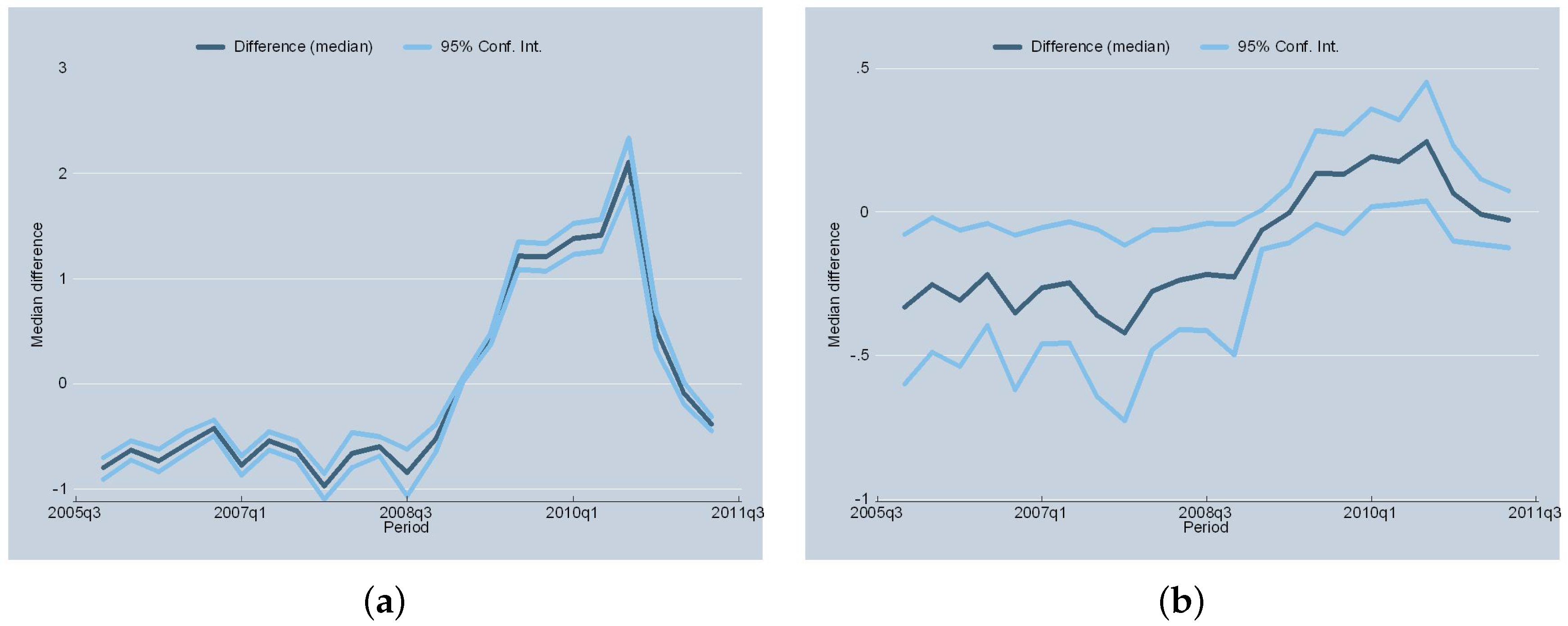
5.5. Simulation Results: When Banks Adhere to the Regulations

We now investigate what is likely to happen once banks actually adhere to the regulations. In the first step, we simulate, for each bank and each period, an optimal balance sheet requiring each bank to adhere to the three Basel III regulations. Banks minimize a loss function subject to the balance sheet, the leverage, LCR and NSFR constraints. The loss function is defined by the profits (multiplied by −1), and as we do not know the true costs of adjusting assets and liabilities,21 we assume that banks face a vector of independently distributed adjustment cost factors (Lucas, Jr 1967; Kopecky and VanHoose 2004). We constrain the adjustment cost terms to be quadratic.22

The result of this simulation exercise is given in

Table 7. Summary statistics: simulated data.

Variable	Mean	Median	SD	Min	Max
Z-score${}_{sim}$	3.708	3.810	0.855	1.735	8.522
ROA${}_{sim}$ *	1.417	1.641	2.778	−5.945	6.775
CAR${}_{sim}$ *	72.526	53.837	67.989	4.029	726.556
TA${}_{sim}$ **	13.527	8.686	14.729	0.284	94.160
OBS${}_{sim}$	0.001	0.000	0.003	0.000	0.024
LCR${}_{sim}$	219.275	100.000	403.724	7.011	5656.088
NSFR${}_{sim}$	2360.512	251.332	8.27$·{10}^5$	100.000	3.03$·{10}^7$
HQLAR${}_{sim}$	0.084	0.051	0.098	0.001	0.731
NOR${}_{sim}$	0.058	0.030	0.074	0.001	0.545
ASFR${}_{sim}$	0.233	0.226	0.128	0.011	0.669
RSFR${}_{sim}$	0.338	0.331	0.175	0.010	0.770

Source: bank-level data, quarterly reporting, authors’ calculations; * in percent; ** billion of euros.

. We find that our simulation predicts that individual banks’ assets increase, on average, by 19%. Furthermore, all new Basel III regulations have a higher mean. Finally, using the simulation outcome and based on our estimates of Equations (2) (Regression (3) of Table 2) and (4) (Regression (9) of Table 4), we predict for each bank and period a “simulated” ROA and Z-score.

As in the econometric estimation, the following analysis considers the global financial crisis and the European debt crisis as exogenous shocks to Luxembourg’s banking sector. Figure 2a,b plots the median difference between the simulated and observed values of, respectively, ROA and the Z-score. Then, positive values indicate that the median bank would have improved its profitability and/or Z-score if it had been complying with Basel III. The dark blue line shows the median difference and the light blue ones the limits of a 90% confidence interval. As can be seen in Figure 2a, the median difference in ROA is significantly negative prior to the global financial crisis and becomes significantly positive in 2009. This result indicates that complying with Basel III is costly and would have implied a reduction of ROA of around 75 basis points in the period previous to the crisis. However, during the crisis, banks in Luxembourg would have experienced higher profits if they would have met the Basel III requirements. The difference reaches 200 basic points by the end of 2010 and declines thereafter.

Figure 2b shows that the evolution of the difference in the Z-score index reflects the ROA results. The difference in the Z-score index is significantly negative before the crisis, though the confidence interval is quite wide, and the upper limit evolves close to zero. After the global financial crisis episode, the difference tends to be not significantly different from zero with just a few quarters showing a positive gap. Indeed, the increases in the capital-to-asset ratio induced by compliance just compensate for the reduction of ROA induced by the impact of the global financial crisis.

Our results tend to support the view of the BCBS, which believes that the new Basel III regulations raise the resilience of banks in periods of potential financial distress. In other words, we expect the LCR, the NSFR and the leverage standards to significantly reduce the expected probabilities of default in Luxembourg’s banking sector. It is worth noting that both the differences in ROA and the Z-score tend to increase during the period covering the global financial crisis and tend to decrease in 2011 during the deepening of the sovereign debt crisis. This suggests that Basel III regulations would tend to improve banks’ resiliency more strongly in liquidity-type crisis periods than in financial crises arising from different underlying problems.

Of course, this result is subject to the Lucas critique. We assume that there is no qualitative change in banks’ behavior once the Basel III regulations are imposed. This is, certainly, not an innocuous assumption. For example, Wagner (2007) shows that higher liquidity increases a bank’s stability as the bank may liquidate assets more easily during a crisis period. However, Wagner (2007) also shows that these banks with higher liquidity are more likely to take on higher risks since the increased liquidity tends to make crises less costly for banks. He concludes that, overall, a banking sector’s stability might actually decrease. Similar results are obtained with respect to capital regulations by Besanko and Kanatas (1996), Lam and Chen (1985), as well as Gennotte and Pyle (1991). Clearly, our empirical study cannot take these second-round effects into account. Nevertheless, we would expect our results to hold as long as the mechanics underlying the return on average assets do not change too much as a consequence of Basel III.

6. Conclusions

In this article, we contribute to the recent discussion on the usefulness and effectiveness of the Basel III regulations by analyzing how the capital-to-assets ratio, the liquidity coverage ratio and the net stable funding ratio are likely to impact banks’ distance-to-default. We used the Z-score index as the indicator of banks’ distance-to-default. We have also studied the components of Z-score, namely ROA and CAR. This approach allows us to account for the endogenous relationship between banks’ profitability and capitalization and then to provide an accurate picture of the potential benefits (i.e., reduced default risk) and costs (i.e., reduced profits) of the Basel III regulations for the Luxembourg case.

We focus on a unique panel dataset based on banks in Luxembourg covering the period 2003q2–2011q3. Our point of departure was the construction of historical series of the banks’ positions with respect to the new Basel III regulations. We then empirically investigated whether historical positions of the LCR and the NSFR components affect banks’ distance-to-default. We focused on the endogenous relationships between ROA, capital-to-assets ratio, the proxies of Basel III standards and other balance-sheet characteristics. For this, we resorted to a GMM type instrumental variables estimator. Our econometric results are robust and rather clear: all of the Basel III regulations that we investigate here will contribute to reducing the risk of default. Thus, we support the view of the BCBS that Basel III is likely to improve banks’ resilience to outside shocks.

We used a numerical model of optimal bank behavior to estimate individual balance sheets for each point in time, constraining banks to adhere to the new regulations. This gives us estimates of the banks’ balance sheets and positions with respect to the Basel III regulations, assuming that these regulations had previously been put in place. We use this simulated data to derive, based on our preferred econometric models, simulated ROA and Z-score series when banks adhere to the regulations. Based on this analysis, we predict that basically all banks would have seen a decrease in their expected defaults during liquidity-type crisis episodes if these banks had previously adhered to the regulations. Thus, we expect that the Basel III regulation will diminish the risk of bank defaults and improve the financial soundness of the banking sector. We also show that the benefits do not go without a cost as adhering to Basel III would have represented a burden of around 75 basic points on banks’ ROA during the period before the global financial crisis.

References

1. Acharya, Viral V., Lasse, H. Pedersen, Philippon Thomas, and Richardson Matthew. 2010. Measuring Systemic Risk. New York: Wiley Online Library. [Google Scholar]
2. Adrian, Tobias, and K. Brunnermeier Markus. 2016. CoVaR. The American Economic Review 106: 1705–41. [Google Scholar] [CrossRef]
3. Adrian, Tobias, and Shin Song Hyun. 2010. Liquidity and leverage. Journal of Financial Intermediation 19: 418–37. [Google Scholar] [CrossRef]
4. Angelini, Paolo, Laurent Clerc, Vasco Cúrdia, Leonardo Gambacorta, Andrea Gerali, Alberto Locarno, Roberto Motto, Werner Roeger, Skander Van den Heuvel, and Jan Vlček. 2011. BASEL III: Long-Term Impact on Economic Performance and Fluctuations. Technical Report. Basel: Bank for International Settlements (BIS). [Google Scholar]
5. Athanasoglou, Panayiotis P., Sophocles N. Brissimis, and Matthaios D. Delis. 2008. Bank-specific, industry- specific and macroeconomic determinants of bank profitability. Journal of International Financial Markets, Institutions and Money 18: 121–36. [Google Scholar] [CrossRef]
6. Arellano, Manuel, and Stephen Bond. 1991. Some tests of specification for panel data: Monte Carlo evidence and an application to employment equations. The Review of Economic Studies 58: 277–97. [Google Scholar] [CrossRef]
7. Arellano, Manuel, and Olympia Bover. 1995. Another look at the instrumental variable estimation of error- components models. Journal of Econometrics 68: 29–51. [Google Scholar] [CrossRef]
8. Blundell, Richard, and Stephen Bond. 1998. Initial conditions and moment restrictions in dynamic panel data models. Journal of Econometrics 87: 115–43. [Google Scholar] [CrossRef]
9. Brownlees, Christian, and Robert F. Engle. 2016. SRISK: A conditional capital shortfall measure of systemic risk. Review of Financial Studies 30: 48–79. [Google Scholar] [CrossRef]
10. BCBS. 2014. Basel III Leverage Ratio Framework and Disclosure Requirements. Technical Report, Bank for International Settlements (BIS). Basel: BCBS (Basel Committee on Banking Supervisors). [Google Scholar]
11. BCBS. 2013. LCR: The Liquidity Coverage Ratio and Liquidity Risk Monitoring Tools. Technical Report, Bank for International Settlements (BIS). Basel: BCBS (Basel Committee on Banking Supervisors). [Google Scholar]
12. BCBS. 2010a. Basel III: International Framework for Liquidity Risk Measurement, Standards and Monitoring. Rules Text, Bank for International Settlements. Basel: BCBS (Basel Committee on Banking Supervisors). [Google Scholar]
13. BCBS. 2010b. Basel III: A Global Regulatory Framework for More Resilient Banks And Banking Systems. Rules Text, Bank for International Settlements. Basel: BCBS (Basel Committee on Banking Supervisors). [Google Scholar]
14. Besanko, David, and George Kanatas. 1996. The regulation of bank capital: Do capital standards promote bank safety? Journal of financial intermediation 5: 160–83. [Google Scholar] [CrossRef]
15. BCBS. 2010. Results of the Comprehensive Quantitative Impact Study. Technical Report, Bank for International Settlements. Basel: BCBS (Basel Committee on Banking Supervisors). [Google Scholar]
16. Berger, Allen N. 1995. The relationship between capital and earnings in banking. Journal of Money, Credit and Banking 27: 432–56. [Google Scholar] [CrossRef]
17. Berger, Allen, Gerald Hanweck, and David B. Humphrey. 1987. Competitive viability in banking: Scale, scope, and product mix economies. Journal of Monetary Economics 20: 501–20. [Google Scholar] [CrossRef]
18. Berger, Allen N., and Christa H. S. Bouwman. 2010. How Does Capital Affect Bank Performance During Financial Crises? Wharton Financial Institutions Center WP 109: 146–76. [Google Scholar]
19. Basurto, Miguel A. Segoviano, and Raphael A. Espinoza. 2011. Probabilities of Default and the Market Price of Risk in a Distressed Economy. IMF Working Paper, April 1. [Google Scholar]
20. Berger, Allen N., Leora F. Klapper, and Rima Turk-Ariss. 2009. Bank competition and financial stability. Journal of Financial Services Research 35: 99–118. [Google Scholar] [CrossRef]
21. Bikker, Jacob A., and Haixia Hu. 2002. Cyclical patterns in profits, provisioning and lending of banks. DNB Staff Reports 55: 143–175. [Google Scholar]
22. Berger, Allen N. 1995. The profit-structure relationship in banking-tests of market-power and efficient-structure hypotheses. Journal of Money, Credit and Banking 27: 404–31. [Google Scholar] [CrossRef]
23. Barth, James R., Gerard Caprio Jr., and Ross Levine. 2004. Bank regulation and supervision: What works best? Journal of Financial Intermediation 13: 205–48. [Google Scholar] [CrossRef]
24. Bourke, Philip. 1989. Concentration and other determinants of bank profitability in Europe, North America and Australia. Journal of Banking & Finance 13: 65–79. [Google Scholar] [CrossRef]
25. Brunnermeier, Markus, Andrew Crockett, Charles Goodhart, Avinash D. Persaud, and Hyun Song Shin. 2009. The Fundamental Principles of Financial Regulation. Technical Report. London: Centre for Economic Policy Research. [Google Scholar]
26. Chrystal, Alec, and Paul D. Mizen. 2003. Goodhart’s Law: Its origins, meaning and implications for monetary policy. In Central Banking, Monetary Theory and Practice: Essays In Honour of Charles Goodhart. Cheltenham: Edward Elgar Publishing. [Google Scholar]
27. Campbell, John Y., Jens Hilscher, and Jan Szilagyi. 2008. In search of distress risk. The Journal of Finance 63: 2899–939. [Google Scholar] [CrossRef]
28. Chan-Lau, Jorge A., and Amadou N. Sy. 2007. Distance-to-default in banking: A bridge too far? Journal of Banking Regulation 9: 14–24. [Google Scholar] [CrossRef]
29. Crouhy, Michel, Dan Galai, and Robert Mark. 2000. A comparative analysis of current credit risk models. Journal of Banking & Finance 24: 59–117. [Google Scholar] [CrossRef]
30. Demirguc-Kunt, Asli, Enrica Detragiache, and Thierry Tressel. 2008. Banking on the principles: Compliance with Basel Core Principles and bank soundness. Journal of Financial Intermediation 17: 511–42. [Google Scholar] [CrossRef]
31. Dietsch, Michel, and Joel Petey. 2002. The credit risk in SME loans portfolios: Modeling issues, pricing, and capital requirements. Journal of Banking & Finance 26: 303–22. [Google Scholar] [CrossRef]
32. Duffie, Darrell, and Jun Pan. 1997. An overview of value at risk. The Journal of Derivatives 4: 7–49. [Google Scholar] [CrossRef]
33. Demirgüç-Kunt, Ash, and Harry Huizinga. 1999. Determinants of commercial bank interest margins and profitability: Some international evidence. The World Bank Economic Review 13: 379–408. [Google Scholar] [CrossRef]
34. Drehmann, Mathias, and Nikola A. Tarashev. 2011. Systemic importance: Some simple indicators. BIS Quarterly Review March: 25–37. [Google Scholar]
35. DeNicolo, Gianni. Size, charter value and risk in banking: An international perspective (April 2001). International Finance Discussion Papers, EFA 2001 Barcelona Meetings. FRB International Finance Discussion Paper No. 689.
36. Duffie, Darrell, and Kenneth J. Singleton. 2003. Credit Risk: Pricing, Measurement, and Management. Princeton: Princeton University Press. [Google Scholar]
37. DeNicolo, Gianni, Jahanara Zaman, Mary G. Zephirin, and Philip F. Bartholomew. 2004. Bank consolidation, internationalization, and conglomeration: Trends and implications for financial risk. Financial Markets, Institutions & Instruments 13: 173–217. [Google Scholar]
38. Giordana, Gaston A., and Ingmar Schumacher. 2013. Bank liquidity risk and monetary policy. Empirical evidence on the impact of Basel III liquidity standards. International Review of Applied Economics 27: 633–55. [Google Scholar] [CrossRef]
39. Giordana, Gaston, and Ingmar Schumacher. 2012. What are the bank-specific and macroeconomic drivers of banks’ leverage? Evidence from Luxembourg. Empirical Economics 45: 1–24. [Google Scholar] [CrossRef]
40. Giordana, Gaston, and Ingmar Schumacher. 2012. An empirical study on the impact of Basel III standards on banks’ default risk: The case of Luxembourg. Banque Centrale du Luxembourg Working Papers 79: 1–31. [Google Scholar]
41. Giordana, Gaston Andres. 2016. Welfare and stochastic dominance for the measurement of banks’ domestic systemic importance: Analytical framework and application. International Journal of Finance and Economics 21: 192–208. [Google Scholar] [CrossRef]
42. Gennotte, Gerard, and David Pyle. 1991. Capital controls and bank risk. Journal of Banking & Finance 15: 805–24. [Google Scholar] [CrossRef]
43. Goddard, John, Phil Molyneux, and John O. S. Wilso. 2004. Dynamics of growth and profitability in banking. Journal of Money, Credit and Banking 36: 1069–90. [Google Scholar] [CrossRef]
44. Goddard, John, Phil Molyneux, and John O. S. Wilson. 2004. The profitability of european banks: A cross-sectional and dynamic panel analysis. The Manchester School 72: 363–81. [Google Scholar] [CrossRef]
45. Gordy, Michael B. 2000. A comparative anatomy of credit risk models. Journal of Banking & Finance 24: 119–49. [Google Scholar]
46. Hamermesh, Daniel S., and Gerard A. Pfann. 1996. Adjustment costs in factor demand. Journal of Economic Literature 34: 1264–92. [Google Scholar]
47. Jackson, Patricia, and William Perraudin. 2000. Regulatory implications of credit risk modelling. Journal of Banking & Finance 24: 1–14. [Google Scholar] [CrossRef]
48. Jin, Xisong, and Francisco Nadal de Simone. 2011. Market and book based models of probability of default for developing macroprudential policy tools. Banque Centrale du Luxembourg, Working Paper, August 29. [Google Scholar]
49. Jin, Xisong, and Francisco Nadal De Simone. 2014. Banking systemic vulnerabilities: A tail-risk dynamic CIMDO approach. Journal of Financial Stability 14: 81–101. [Google Scholar] [CrossRef]
50. Judson, Ruth A., and Ann Owen. 1999. Estimating dynamic panel data models: A guide for macroeconomists. Economics Letters 65: 9–15. [Google Scholar] [CrossRef]
51. Kopecky, Kenneth J., David Vanhoose, K. Kopecky, and D. VanHoose. 2004. A model of the monetary sector with and without binding capital requirements. Journal of Banking & Finance 28: 633–46. [Google Scholar] [CrossRef]
52. Lam, Chun H., and Andrew H. Chen. 1985. Joint effects of interest rate deregulation and capital requirements on optimal bank portfolio adjustments. Journal of Finance 40: 563–75. [Google Scholar] [CrossRef]
53. Lucas, Robert E., Jr. 1976. Econometric policy evaluation: A critique. In Carnegie-Rochester Conference Series on Public Policy. New York: Elsevier, vol. 1, pp. 19–46. [Google Scholar]
54. Lucas, Robert E., Jr. 1967. Adjustment costs and the theory of supply. The Journal of Political Economy 75: 321–34. [Google Scholar] [CrossRef]
55. Maechler, Andrea M., Srobona Mitra, and Delisle Worrell. 2007. Decomposing financial risks and vulnerabilities in Eastern Europe. IMF Working Paper WP/07/ 248: 1–33. [Google Scholar]
56. Merton, Robert C. 1974. On the pricing of corporate debt: The risk structure of interest rates. The Journal of Finance 29: 449–70. [Google Scholar] [CrossRef]
57. Moore, Kyle, and Chen Zhou. 2013. ‘Too Big to Fail’ or ‘Too Non-Traditional to Fail?’ The Determinants of Banks’ Systemic Importance. MPRA Paper 45589. Munich: University Library of Munich. [Google Scholar]
58. Molyneux, Philip, and John Thornton. 1992. Determinants of European bank profitability: A note. Journal of Banking & Finance 16: 1173–78. [Google Scholar] [CrossRef]
59. Nickell, Stephen. 1981. Biases in dynamic models with fixed effects. Econometrica: Journal of the Econometric Society 49: 1417–26. [Google Scholar] [CrossRef]
60. Richard, Podpiera. 2006. Does Compliance with Basel Core Principles Bring Any Measurable Benefits? IMF Staff Papers 53: 306–25. [Google Scholar]
61. Ronald, Anderson, and Suresh Sundaresan. 2000. A comparative study of structural models of corporate bond yields: An exploratory investigation. Journal of Banking & Finance 24: 255–69. [Google Scholar]
62. Smirlock, Michael. 1985. Evidence on the (non) relationship between concentration and profitability in banking. Journal of Money, Credit and Banking 17: 69–83. [Google Scholar] [CrossRef]
63. Slovik, Patrick, and Boris Cournède. 2011. Macroeconomic Impact of Basel III. OECD Economics Department Working Papers, February 14. [Google Scholar]
64. Segoviano, Miguel, and Charles Goodhart. 2009. Banking stability measures. IMF Working Paper, January 1. [Google Scholar]
65. Tarashev, Nikola, Claudio Borio, and Kostas Tsatsaronis. 2009. The systemic importance of financial institutions. BIS Quarterly Review September: 75–87. [Google Scholar]
66. Tarashev, Nikola, Claudio Borio, and Kostas Tsatsaronis. 2010. Attributing systemic risk to individual institutions. BIS Working Paper 308: 1–29. [Google Scholar] [CrossRef]
67. Wagner, Wolf. 2007. The liquidity of bank assets and banking stability. Journal of Banking & Finance 31: 121–39. [Google Scholar] [CrossRef]
68. Wolff, Christian C. P., and Nikolaos I. Papanikolaou. 2015. Leverage and Risk in US Commercial Banking in the Light of the Current Financial Crisis. CEPR Discussion Paper DP10890: 1–27. [Google Scholar]
69. Windmeijer, Frank. 2005. A finite sample correction for the variance of linear efficient two-step GMM estimators. Journal of econometrics 126: 25–51. [Google Scholar] [CrossRef]
70. Zhou, Chen. 2010. Are banks too big to fail? Measuring systemic importance of financial institutions. International Journal of Central Banking 6: 205–50. [Google Scholar] [CrossRef]
1.
The BCBS is an international committee constituted by central bank representatives from all around the world and other banking supervisory authorities. It has no legally-binding authority, but provides an international forum of discussion for guidelines and rules for banking supervision that local authorities may implement.
2.
The Z-score index of banks in Luxembourg is calculated by the Central Bank of Luxembourg. Aggregated figures are published annually in the Financial Stability Review.
3.
This dataset is confidential and cannot be distributed. Other available datasets provide a level of granularity far below the one required for a consistent estimate of both ratios.
4.
See Chrystal and Mizen (2003). Goodhart’s law is intimately related to Lucas’ critique formulated later (see Lucas (1976)).
5.
One can find measures based on theoretical models or, alternatively, indicator-based ones that result from aggregating bank-level variables related to the systemic relevance of banks. Some model-based measures are aimed at quantifying the contribution of individual institutions to systemic risk (e.g. Tarashev et al. 2009; Tarashev et al. 2010; Acharya et al. 2010; Adrian and Brunnermeier 2016; Brownlees and Engle 2016). Others focus on interconnectedness externalities (e.g., Segoviano and Goodhart 2009; Zhou 2010; Jin and Nadal De Simone 2014)).
6.
Giordana 2016 shows that indicator-based measures of systemic importance that account for the balance sheet size of banks would increase the welfare gains of capital surcharges.
7.
Other related proxies are Moody’s financial strength ratings (e.g., Demirgüç-Kunt et al. 2008); Merton-KMV model (e.g., Merton 1974; Anderson and Sundaresan 2000); default-mode models (e.g., Dietsch and Petey 2002); value-at-risk models (e.g., Duffie and Pan 1997). For a survey, see Crouhy et al. 2000; for a discussion, see Jackson and Perraudin (2000); for a comparison, see Gordy (2000).
8.
There are no institutions in Luxembourg’s banking sector with stock market quotation.
9.
“Market liquidity is low when it is difficult to raise money by selling the asset at reasonable prices. In other words, market liquidity is low when selling the asset depresses the sale price. When market liquidity is low, it is very costly to shrink a firm’s balance sheet” (Brunnermeier et al. 2009, p. 14).
10.
“Funding liquidity describes the ease with which investors can obtain funding from financiers. Funding liquidity is high when it is easy to raise money” (Brunnermeier et al. 2009, p. 14).
11.
Then, CAR i t is correlated with ϵ 1 , i t 1 and earlier shocks, but is uncorrelated with ϵ 1 , i t and subsequent shocks.
12.
This implies that ROA i t is correlated with ϵ 2 , i t and earlier shocks, but is uncorrelated with ϵ 2 , i t + 1 and future shocks.
13.
As an indicator of credit risk, we also considered the ratio of provisions-to-loans. We did not not retain it in the final specification since the coefficient was not statistically significant.
14.
The fifth column of Table 5 provides definitions for the coefficients β ’s in Equation (4).
15.
The dynamic-panel bias is introduced through correlation between the lagged dependent variable and the fixed effects (Nickell 1981).
16.
The Z-score specification encompasses a proper AR(1) process if it is assumed that β 1 = β 2
17.
We use the “nlsur” command in Stata 11.
18.
A previous version of this study (Giordana and Schumacher 2012) makes use of the previous LCR definition (see BCBS 2010a). The LCR picture is quite different.
19.
In order to improve the rendering of the estimation results table, ROA and CAR has been multiplied by 100 (in percentage points) when performing the estimation.
20.
There is no clear prediction on the sign of the size-profit relationship. While size certainly accounts for economies or dis-economies of scale, it can be correlated with various financial, legal and political factors that may affect profitability. The empirical evidence is not clear either. For instance, Smirlock (1985) finds a positive and significant relationship while Berger et al. (1987), among others, suggest that increasing the size allows for little cost saving. In a more recent European cross-country study, Goddard et al. (2004) do not find convincing evidence for any consistent or systematic relationship between size and profitability. Likewise, Athanasoglou et al. (2008) show that the effect of bank size on profitability is not important.
21.
Indeed, these costs could be direct and indirect, ranging from haircuts when selling the assets to potential reputation damage.
22.
For a discussion, see Hamermesh and Pfann (1996). The complete simulation model is described in detail in Giordana and Schumacher (2013).
Figure 1. Evolution of main variables, 2003q2–2011q3. (a) Evolution of the Z-score, 2003q2–2011q3; (b) evolution of ROA and CAR, 2003q2–2011q3; (c) evolution of LCR, 2003q2–2011q3; (d) evolution of NSFR, 2003q2–2011q3.
Jrfm 10 00008 g001
Figure 2. Comparison of simulated versus observed ROA and the Z-score. (a) Median difference between simulated and observed ROA; (b) median difference between simulated and observed Z-score.
Jrfm 10 00008 g002