Reconstruction Optimization Algorithm of 3D Temperature Distribution Based on Tucker Decomposition

Abstract

For the purpose of solving the large temperature field reconstruction error caused by different measuring point arrangements and the problem that the prior dataset cannot be built due to data loss or distortion in actual measurement, a three-dimensional temperature profile reconstruction optimization algorithm is proposed to repair the empirical dataset and optimize the arrangement of temperature measuring points based on Tucker decomposition, the minimum condition number method, the greedy algorithm, and the hill climbing algorithm. We used the Tucker decomposition algorithm to repair the missing data and obtain the complete prior dataset and the core tensor. By optimizing the dimension of the core tensor and the number and position of the measuring points calculated by the minimum condition number method, the greedy algorithm, and the mountain climbing algorithm, the real-time three-dimensional distribution of the temperature field is reconstructed. The results show that the Tucker decomposition optimization algorithm could accurately complete the prior dataset, and compared with the original algorithm, the proposed optimal placement algorithm improves the reconstruction accuracy by more than 20%. At the same time, the algorithm has strong robustness and anti-noise, and the relative error is less than 4.0% and 6.0% with different signal-to-noise ratios. It indicates that the proposed method can solve the problem of building an empirical dataset and 3D temperature distribution reconstruction more accurately and stably in industry.

1. Introduction

Industrial temperature data tend to be large and contain a lot of redundant information and noise. At the same time, under different working conditions in industry, the flame in the furnace has different temperature distributions and flame offset phenomena. With the rapid growth of the amount of data and the continuous maturity of computer technology, obtaining the ability to perform new tasks by analyzing and identifying historical data has gradually become a research hotspot. With this demand, machine learning has developed rapidly. At present, machine learning has become a powerful tool for natural language processing, image recognition, image reconstruction, data mining, etc. [1]. It can integrate the advantages of measurement methods and numerical methods to reconstruct the temperature distribution.

Tucker decomposition is a classical machine learning algorithm first proposed by Tucker in 1963 [2]. Tucker decomposition is widely used in large-scale data processing, such as recognition [3], picture processing [4], signal processing [5], and so on. Karami et al. [6] used the kernel trick to apply Tucker decomposition on a higher dimensional feature space for the denoising of hyperspectral images. Zhang et al. [7] propose a robust human action recognition algorithm by tensor representation and Tucker decomposition, using the Tucker tensor decomposition to decompose the unknown tensor parameter, and then using the alternative optimization method to solve the optimization problems. Zhao et al. [8] used it to detect infrared small targets and estimate and eliminate the major principal components, enhancing the image contrast. In previous studies, we have reconstructed the three-dimensional temperature field by Tucker decomposition [9]. Although the temperature field distribution can be obtained by the Tucker decomposition reconstruction algorithm through a small amount of measurement data, different arrangements of measuring points have a great influence on the reconstruction accuracy due to the small amount of measurement data. At the same time, industrial data often have missing or distorted phenomena, resulting in incomplete empirical datasets, which cannot be directly reconstructed using the reconstruction algorithm proposed by the author before [9]. Most existing research, however, focused on how to use Tucker decomposition to analyze flow field distribution and image reconstruction, ignoring the establishment of empirical datasets and the selection of optimal measurement points. Qin et al. [10] used it for wind field reconstruction predictions and to create a third-order prior database by CFD simulations. Hou et al. [11] obtained the optimal parameter through the energy-cumulative method that computes the sum of eigenvalues one by one. This method cannot automatically select eigenvalues, and they must be manually added one by one until the cumulative energy achieves a specified ratio to all energy when using Tucker decomposition in hyperspectral change detection. Generally, Tucker decomposition can be regarded as high-order principal component analysis (PCA) [12]. The PCA can be used to complete the missing dataset, and the temperature distribution can be reconstructed by extracting the basis vector from the completed dataset. Everson and Sirovich first applied this algorithm to image processing [13] and achieved good results. Therefore, in the absence of empirical data, using the optimizing reconstruction algorithm to explore the temperature field can further improve the robustness and generalization ability of the algorithm.

The work presented in this paper is part of a continuing effort following previous attempts based on the 3D Tucker decomposition reconstruction algorithm [9]. This study optimizes the applicability of the Tuck decomposition algorithm to reconstruct the temperature field in the absence of a prior dataset. In the research process, the missing position of the original dataset and the position and number of the measuring point during the reconstruction process have a great influence on the reconstruction error, indicating that the information carried by different measuring point positions is different in the temperature distribution reconstruction algorithm. Therefore, this paper optimizes the arrangement of measuring points and adds Gaussian noise to the measured values by simulating the actual measurement process. The reconstruction results are compared with the actual temperature field to evaluate the reliability of the proposed technical method.

2. Fundamental Measurement Principles

2.1. Tucker Decomposition Reconstruction Algorithm

The following is a brief introduction to the Tucker decomposition reconstruction algorithm. The detailed derivation process is shown in the previously published paper [9].

A prior dataset obtained by simulation calculations or by sensors is denoted as $\mathit{T}\mathit{R}=\left\{{\mathit{T}}_1,{\mathit{T}}_2,{\mathit{T}}_3,\dots ,{\mathit{T}}_i,\dots ,{\mathit{T}}_{n1}\right\}, {\mathit{T}}_i\in {\complement }^{n_2\times n_3\times n_4},\mathit{T}\mathit{R}\in {\complement }^{n_1\times n_2\times n_3\times n_4}$. Through Tucker decomposition and tensor properties, the prior dataset can be decomposed into the following form:

$$\mathit{T}\mathit{R}=\left\{\begin{array}{c}{\mathit{T}}_1\\ {\mathit{T}}_2\\ \begin{array}{c}⋮\\ {\mathit{T}}_i\\ \begin{array}{c}⋮\\ {\mathit{T}}_{n_1}\end{array}\end{array}\end{array}\right\}={\mathit{C}}_t{\times }_1\mathit{F}{\times }_2{\mathit{V}}_{}{\times }_3{\mathit{W}}_{}{\times }_4\mathit{U},$$

(1)

where ${\mathit{C}}_t\in {\complement }^{m_1\times m_2\times m_3\times m_4} \mathrm{is} \mathrm{called} \mathrm{the} \mathrm{core} \mathrm{tensor}$,$\mathit{U}\in {\complement }^{n_i\times m_i}$,$\mathit{V}\in {\complement }^{n_i\times m_i}$,$\mathit{W}\in {\complement }^{n_i\times m_i}$ and $\mathit{F}\in {\complement }^{n_i\times m_i}$ are four factor matrices.

Because the tensor mode product conforms to this formula $\mathit{C}{\times }_1\mathit{P}{\times }_2\mathit{Q}=\mathit{C}{\times }_2\mathit{Q}{\times }_1\mathit{P}$ [14], Formula (1) can be converted to the following form.

$$\mathit{T}\mathit{R}=\left\{\begin{array}{c}{\mathit{T}}_1\\ {\mathit{T}}_2\\ \begin{array}{c}⋮\\ {\mathit{T}}_i\\ \begin{array}{c}⋮\\ {\mathit{T}}_{n_1}\end{array}\end{array}\end{array}\right\}={\mathit{C}}_t{\times }_2\mathit{V}{\times }_3\mathit{W}{\times }_4\mathit{U}{\times }_1\left\{\begin{array}{c}{\mathit{f}}_{11}\\ {\mathit{f}}_{12}\\ \begin{array}{c}⋮\\ {\mathit{f}}_{1i}\\ \begin{array}{c}⋮\\ {\mathit{f}}_{1n_1}\end{array}\end{array}\end{array}\right\},$$

(2)

where ${\mathit{f}}_{1i}\in {\complement }^{1\times m_1}$ is the ith factor vector in the decomposition factor matrix in the 1 norm direction.

From Formula (2), for the reconstruction under the same conditions, the temperature field should satisfy Formula (3):

$${\mathit{T}}_x=\mathit{A}{\times }_1{\mathit{f}}_{1x},$$

(3)

According to the definition of the pattern product, Formula (3) can be converted to:

$${\mathit{t}}_x={\left({\mathit{f}}_{1x}\times {\mathit{A}}_{1\mathrm{unfold}}\right)}^{\mathrm{T}},$$

(4)

where ${\mathit{t}}_x$ is the representation of the 3D temperature distribution by vector; ${\mathit{A}}_{1\mathrm{unfold}}\in {\complement }^{\left(n_2\times n_3\times n_4\right)\times m_1}$ is the coefficient matrix of $\mathit{A}$ expanding in the direction of 1 mode.

In the process of temperature measurement, when the sensor is arranged, the measurement matrix is determined:

$${\mathit{t}}_{\mathrm{M}}=\mathit{M}{\mathit{t}}_x,$$

(5)

where ${\mathit{t}}_{\mathrm{M}}\in {\mathit{R}}^{k\times 1}$ is a column vector of temperature values measured by the sensor; $\mathit{M}\in {\mathit{R}}^{k\times n}$ denotes sensor position.

It can be derived from Equations (4) and (5):

$$\mathit{M}{\mathit{A}}_{1\mathrm{unfold}}{\mathit{f}}_{1x}^{\mathrm{T}}={\mathit{t}}_{\mathrm{M}},$$

(6)

In Formula (6), ${\mathit{t}}_{\mathrm{M}}$ is the measured value, $\mathit{M}$ is a known matrix, and ${\mathit{A}}_{1\mathrm{unfold}}$ is calculated by Tucker decomposition. Therefore, the solution becomes to establish a reconstruction error minimization function:

$$J\left({\mathit{f}}_{1x}^{\mathrm{T}}\right)=\arg min\Vert {\mathit{t}}_{\mathrm{M}}-\mathit{M}{\mathit{A}}_{1\mathrm{unfold}}^{\mathrm{T}}{\mathit{f}}_{1x}^{\mathrm{T}}{\Vert }^2,$$

(7)

where $J\left({\mathit{f}}_{1x}^{\mathrm{T}}\right)$ is the objective function.

It can be seen from Formula (7) that the temperature distribution reconstruction problem can be transformed into the optimal solution problem of solving the reconstruction coefficient vector:

$$\mathit{B}{\mathit{f}}_{1x}^{\mathrm{T}}=\mathit{k},$$

(8)

where $\mathit{B}={\left(\mathit{M}{\mathit{A}}_{1\mathrm{unfold}}^{\mathrm{T}}\right)}^{\mathrm{T}}\left(\mathit{M}{\mathit{A}}_{1\mathrm{unfold}}^{\mathrm{T}}\right)$; $\mathit{k}={\left(\mathit{M}{\mathit{A}}_{1\mathrm{unfold}}^{\mathrm{T}}\right)}^{\mathrm{T}}{\mathit{t}}_{\mathrm{M}}$.

The distribution of the temperature field can be obtained by solving the above equation and substituting the result into Formula (4).

2.2. Missing Datasets Reconstruction Algorithm

The actual measurement results in industry often have data missing or data distortion, so the measured dataset is generally incomplete and cannot directly use the above reconstruction algorithm. Therefore, one must use the optimization algorithm to repair the missing dataset and then extract the core tensor from the completed prior dataset to realize the 3D temperature distribution reconstruction.

The steps of the 3D temperature optimization reconstruction algorithm for prior datasets with missing data are as follows.

• A prior dataset ${\mathit{G}}_{n_1\times n_2\times n_3\times n_4}\left({\mathit{g}}_1,{\mathit{g}}_2,\cdots ,{\mathit{g}}_i,\cdots ,{\mathit{g}}_{n_1}\right)$ with temperature loss is obtained, where ${\mathit{g}}_i\left(1\le i\le n_1\right)$ represents a three-dimensional temperature distribution with missing data at different locations under various operating conditions;
• Average the temperature of ${\mathit{G}}_{n_1\times n_2\times n_3\times n_4}\left({\mathit{g}}_1,{\mathit{g}}_2,\cdots ,{\mathit{g}}_i,\cdots ,{\mathit{g}}_{n_1}\right)$ in the 1-mode direction, and use the average to complete the missing temperature data in the 1-mode direction vector;
• The dataset after completion is denoted as ${\mathit{G}}^0$, and the core tensor ${\mathit{C}}_t^0$ and the corresponding reconstruction coefficient tensor ${\mathit{A}}_{1\mathrm{unfold}}^0$ along the 1-mode direction are calculated by Tucker decomposition. The ${\mathit{A}}_{1\mathrm{unfold}}^0$ and the original actual measurement data are substituted into the reconstruction algorithm to calculate the coefficient 1-mode decomposition factor vector ${\mathit{f}}_{1x}^0$. The temperature field in the missing dataset is reconstructed by using ${\mathit{A}}_{1\mathrm{unfold}}^0$ and ${\mathit{f}}_{1x}^0$ to complete the missing data in $\mathit{G}$ with the calculated results;
• The dataset completed by step 3 is denoted as ${\mathit{G}}^1$, and the tucker algorithm is used to calculate the core tensor ${\mathit{C}}_t^1$ and the corresponding reconstruction coefficient tensor ${\mathit{A}}_{1\mathrm{unfold}}^1$ expanded along the 1-mode direction. If $\Vert {\mathit{C}}_t^1-{\mathit{C}}_t^0{\Vert }_{\infty }\le {10}^{-3}$, the iterative convergence is determined. If it does not converge, continue to put ${\mathit{A}}_{1\mathrm{unfold}}^1$ and the actual measurement data before the completion into the reconstruction algorithm to calculate the coefficient 1-modulus decomposition factor vector ${\mathit{f}}_{1x}^1$, and use ${\mathit{A}}_{1\mathrm{unfold}}^1$ and ${\mathit{f}}_{1x}^1$ to reconstruct the temperature field distribution in the missing dataset. The missing data in $\mathit{G}$ are completed by the calculated values, and the completed dataset is recorded as ${\mathit{G}}^2$;
• Repeat calculation in step 4 until the convergence conditions are met;
• Taking the m^th iteration dataset ${\mathit{G}}^m$, which satisfies the convergence condition as the final complement prior dataset, the three-dimensional temperature field is reconstructed by ${\mathit{G}}^m$.

The flow diagram of prior dataset completion is shown in the Figure 1.

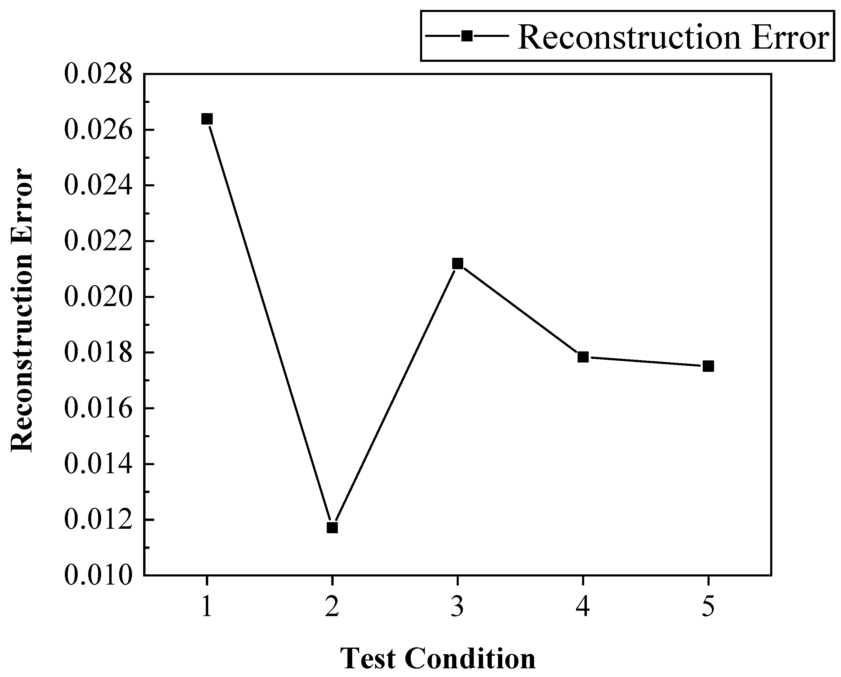
2.3. Reconstruction Result Error

The correlation error $e$ for evaluating reconstruction results is defined as follows.

$$e=\frac{\Vert {\mathit{t}}_x-\mathit{t}{\Vert }_2}{\Vert \mathit{t}{\Vert }_2}$$

(9)

3. Verification and Analysis Based on Numerical Simulation

Set the computational domain of a 3D temperature field to 4 m × 4 m × 4 m. Set the X-axis and Y-axis as 0.1 m as the step length; select four different heights, respectively, 0.5 m, 1.5 m, 2.5 m, and 3.5 m, for the two-dimensional temperature distribution section to characterize the three-dimensional temperature field distribution data. Calculate 4 × 40 × 40 temperature values to establish the three-dimensional temperature distribution data. The Tucker decomposition reconstruction optimization algorithm proposed in this paper is used to reconstruct and calculate the temperature profiles under different experimental conditions and different flame offset situations with data loss and noisy signals. The reconstruction result is analyzed to demonstrate the effectiveness of the Tucker decomposition optimization algorithm and the feasibility of applying the Tucker decomposition algorithm to the reconstruction of three-dimensional temperature distribution with different conditions and different flame deflection.

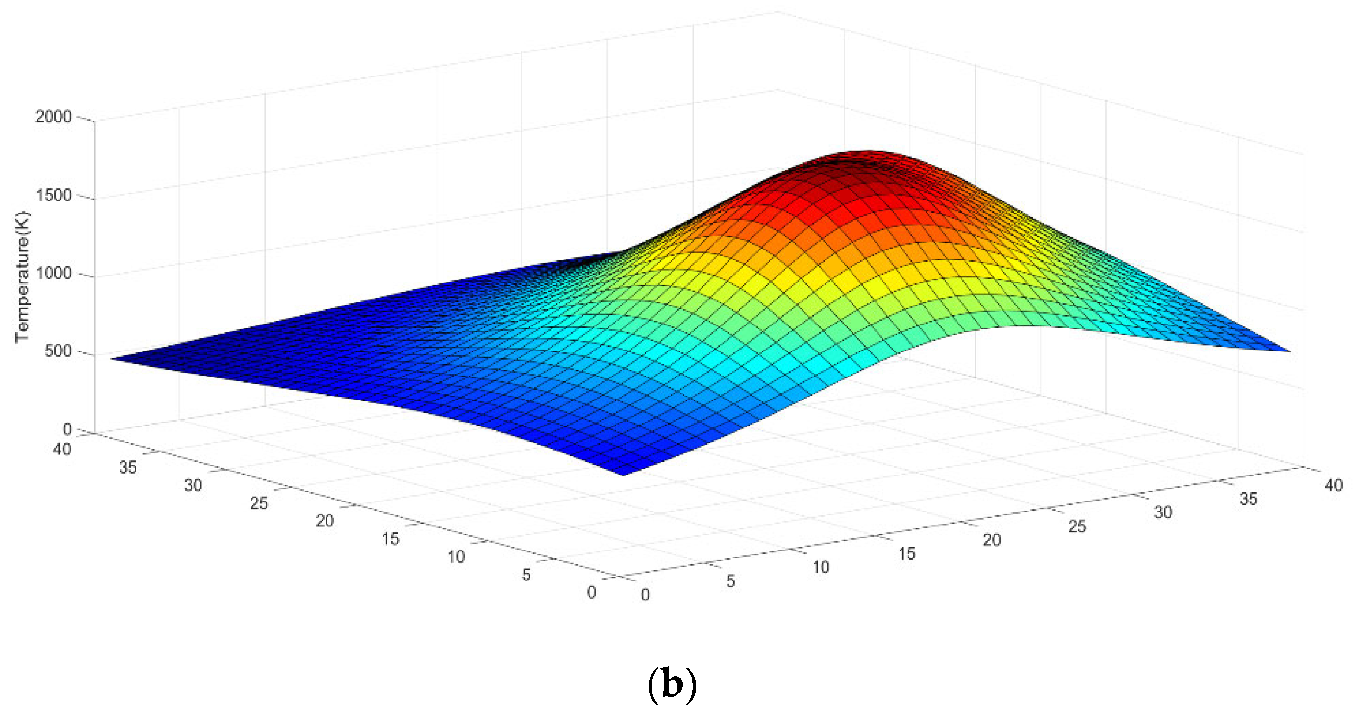
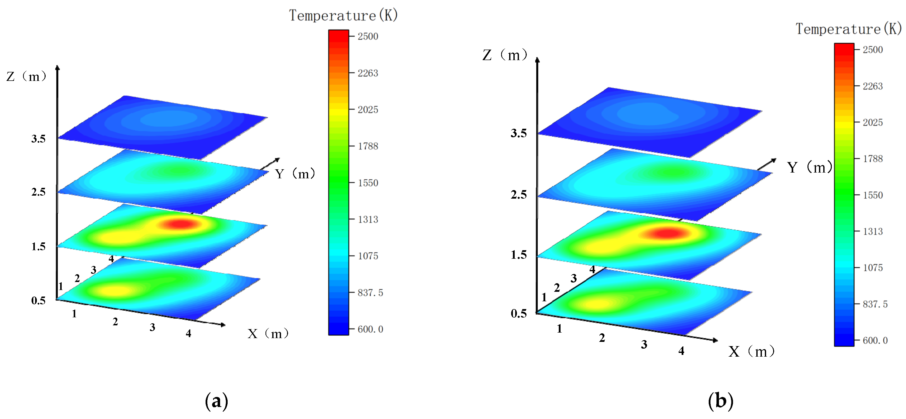
3.1. Temperature Distribution Reconstruction and Simulation Condition Setting

The bimodal temperature distribution is as follows.

$$\mathit{T}\left(x,y,z\right)=270+\frac{a}{{(x-c)}^2+{(y-1)}^2+{(z-1)}^2+1}+\frac{b}{{(x-d)}^2+{(y-2)}^2+{(z-1.5)}^2+1} ,$$

(10)

where $\mathit{T}\left(x,y,z\right)$ is the temperature value of points $\left(x,y,z\right)$ (K); and $a,b,c,d$ are the initial boundary condition; $a,b$ represents different working conditions, and $c,d$ represents the flame center position, controlling the flame deflection degree.

The boundary conditions of the empirical dataset are set as follows: $a,b\in \left[800, 1800\right],c,d\in \left[0,4\right]$. Set (900 + 5) groups of different boundary conditions. The temperature distribution data under different conditions are calculated, and a prior dataset with dimensions of 900 × 4 × 40 × 40 and a test dataset with dimensions of 5 × 4 × 40 × 40 are established. Two typical temperature field distributions with different boundary conditions are randomly selected from 900 sets. The two-dimensional temperature distributions with a height of 1.5 m are interpreted as Figure 2, and the boundary conditions of the test dataset are set as

Table 1. Boundary conditions of test dataset.

Working Condition	Boundary Condition (a)	Boundary Condition (b)	Boundary Condition (c)	Boundary Condition (d)
Test Condition 1	821	1159	0.6	1.5
Test Condition 2	1394	1569	1.1	2.2
Test Condition 3	1521	17.7	2.5	3.6
Test Condition 4	1777	1353	3.5	2.8
Test Condition 5	1827	1973	1.2	3.1

.

3.2. Data Analysis and Discussion

According to the calculation process of three-dimensional temperature profile reconstruction, the reconstruction coefficient matrix is obtained by the tensor decomposition of the prior data. The temperature values of 30 measuring points are preliminarily determined as the temperature measurement data. The core tensor with dimensions of 9 × 4 × 5 × 3 is used to reconstruct 1000 times repeatedly. The error of 1000 reconstruction results of test condition 5 is as follows (Test condition 5’s boundary conditions are outside the data in the dataset):

It can be seen from Figure 3 that the reconstruction errors of different measuring points are very different. The temperature field results calculated by test condition 5 and the temperature distribution results with 1.75% obtained by reconstruction are shown in Figure 4.

As shown in Figure 4, the reconstruction result after preliminary selection can reconstruct the temperature field well, but this result is one of the smaller relative errors selected from the 1000 reconstructions with the different arrangements of measuring points. In order to ensure the high-precision reconstruction of the temperature field, it is necessary to further improve the accuracy on the basis of the first reconstruction calculation and to determine the number and location of the measuring points.

In order to analyze the adaptability of the reconstruction algorithm to different operating conditions, five different operating conditions were calculated with other conditions being equal. Reconstruction error is shown in Figure 5.

It can be seen from Figure 5 that, under the same calculation conditions, the error of test condition 1 is relatively large and the error of test condition 2 is small because of the different boundary conditions. In the calculation domain, the flame of test condition 1 is more inclined to the boundary, while the flame of test condition 2 is relatively located in the center of the calculation domain. Therefore, in practical engineering applications, the reconstruction error of large eccentric flames is relatively large.

The analysis of Figure 3, Figure 4 and Figure 5 shows that the proposed algorithm can effectively reconstruct the temperature distribution under different conditions of the bimodal three-dimensional temperature distribution model. However, it is necessary to optimize the number and arrangement of the measuring points.

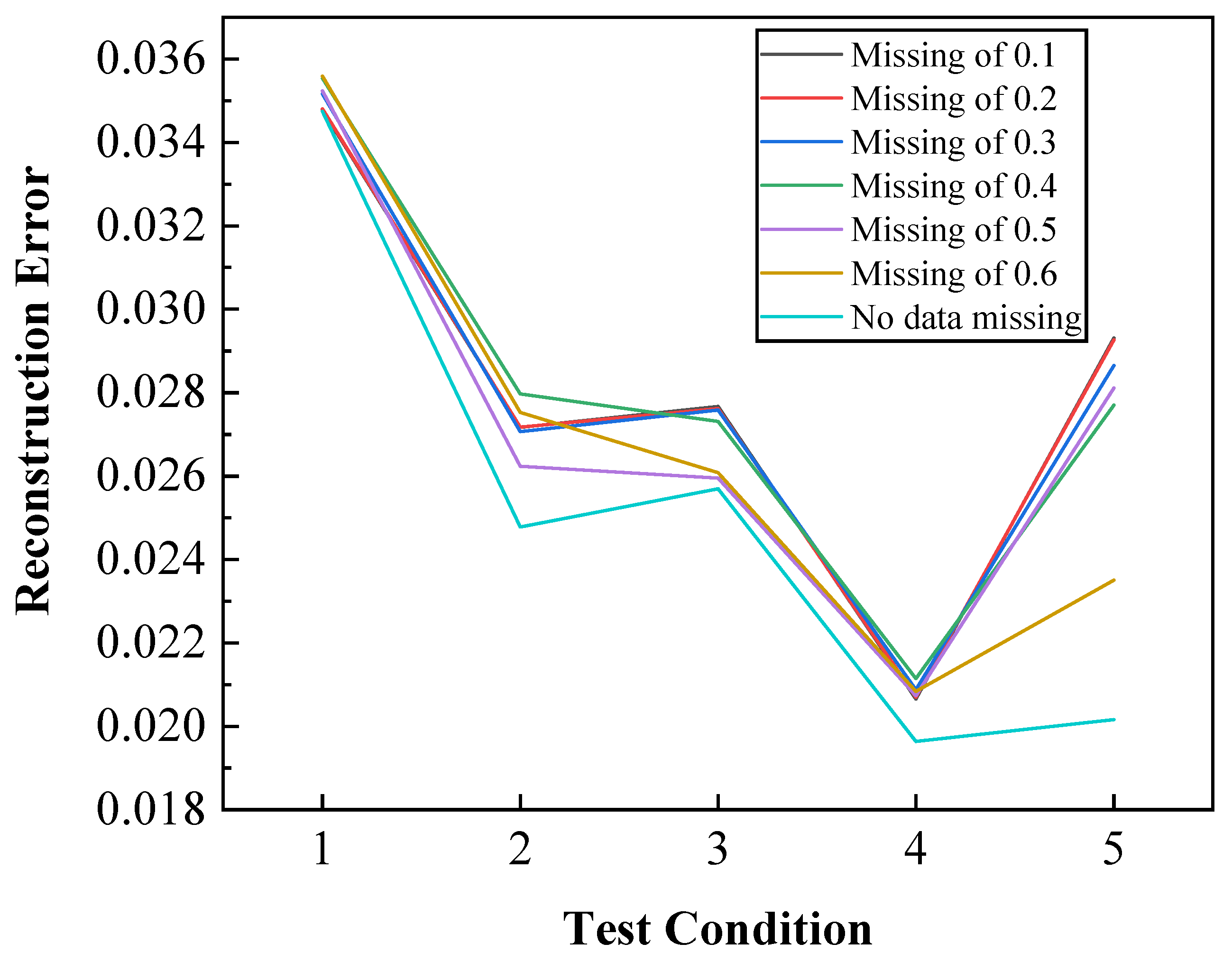
3.3. Temperature Distribution Reconstruction with Data Missing

The original dataset ${\mathit{T}}_{900\times 4\times 40\times 40}$ of the bimodal temperature distribution is processed with data missing, and the missing position is random. The temperature missing dataset is obtained and denoted as ${\mathit{G}}_{900\times 4\times 40\times 40}$. The missing position data in $\mathit{G}$ is replaced by 0, and the remaining data are unchanged.

The temperature missing dataset $\mathit{G}$ is complemented by the reconstruction optimization algorithm, and the core tensor of the complemented dataset is extracted and reconstructed with 13 temperature measuring points. Due to the random data missing, five groups of test datasets of bimodal temperature distributions are reconstructed for many times, and the average reconstruction error is calculated. The reconstruction errors of different missing ratios are shown in Figure 6.

As shown in Figure 6, the results show that the temperature distribution reconstruction algorithm based on Tucker decomposition and missing datasets can also be applied to the reconstruction after completing different proportions of missing datasets, and good reconstruction results are obtained. The reconstruction error of temperature distribution in the five groups of test conditions is less than 3.6 %. Observing the curve trend in the figure, it can be seen that as the data loss rate decreases, the overall reconstruction error also tends to decrease. The blue line is the temperature profile reconstruction error on the basis of the complete dataset. It is observed that the trend of the temperature distribution reconstruction error curve based on the missing dataset is basically consistent with it. Therefore, the temperature reconstruction optimization algorithm of the Tucker decomposition using the prior dataset with temperature missing can accurately complete the incomplete datasets and then achieve the temperature field reconstruction.

4. Reconstruction Parameters Optimization of Tucker Decomposition

When using the algorithm proposed in this paper, it is found that the core tensor dimension of the transformation matrix, the number of measuring points, and the arrangement of measuring points will affect the reconstruction accuracy. Therefore, optimizing the key parameters in the reconstruction calculation process is of great significance to improve the accuracy of the reconstruction algorithm.

4.1. Influence of Core Tensor Dimension

In the previously published article, the dimension of the core vector was been optimized [9]. This paper uses this calculation method to determine the core tensor dimension of 9 × 4 × 5 × 3. Using the optimized core tensor, the data under five experimental conditions are reconstructed, and the effect of the existence of noise with SNR = 20 dB is analyzed. The results are shown in Figure 7.

It can be seen from Figure 7 that under the five test conditions, the optimization effect of the core tensor dimension is equally applicable to the measurement with or without noise. The optimized reconstruction algorithm has high reconstruction accuracy and good noise immunity.

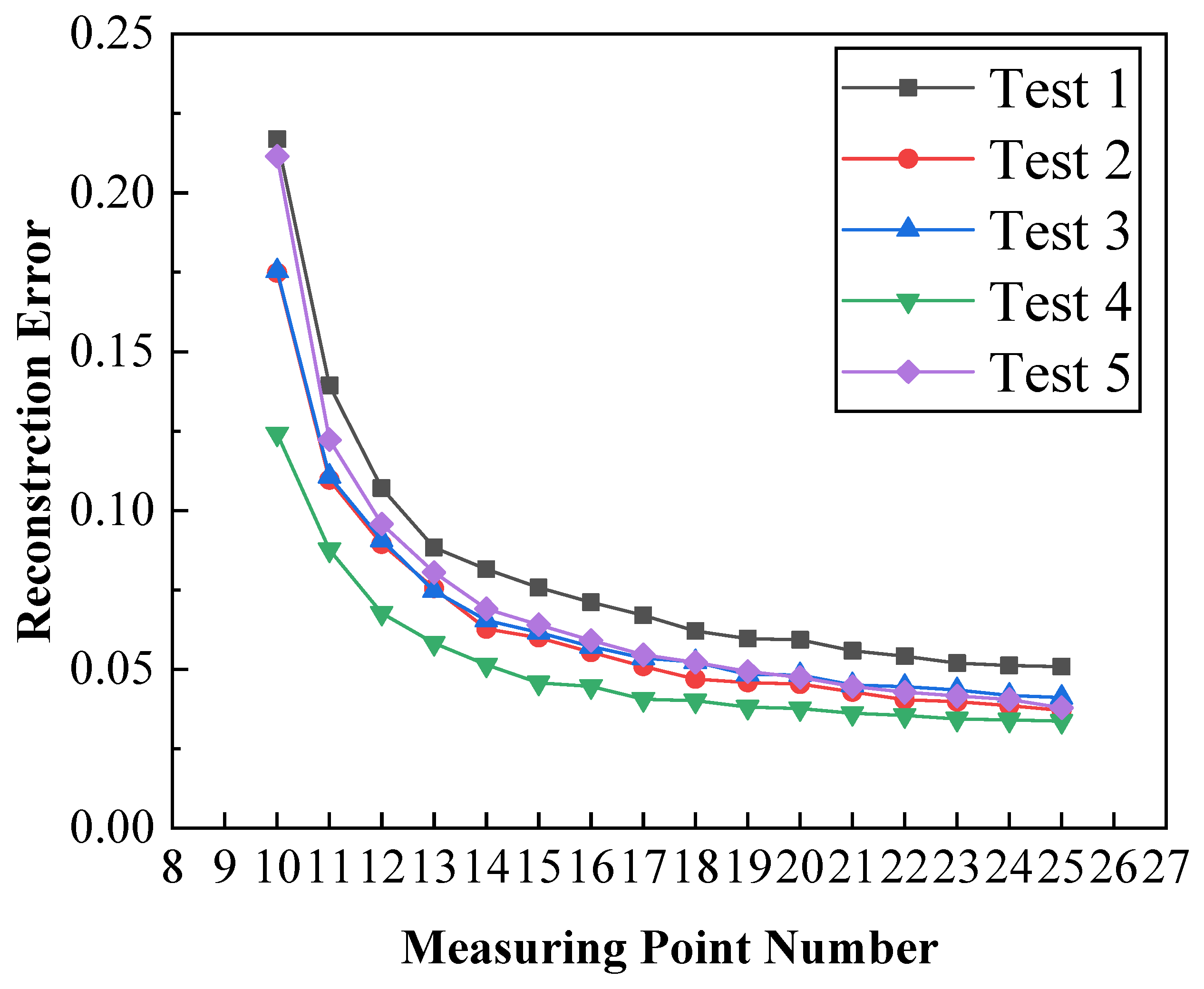
4.2. Effect of Measuring Point Number

The analysis of the reconstruction optimization algorithm shows that the temperature measurement information is the key to establishing a prior dataset and the temperature distribution to be reconstructed. The number of measuring points directly affects the accuracy of temperature field reconstruction. The goal of this paper is to establish a new method to reconstruct the temperature distribution quickly and accurately by using a small amount of temperature measurement data. Therefore, it is important to explore the influence of the number of measuring points on the initial reconstruction accuracy of the algorithm.

Therefore, combined with the optimization results of the core tensor dimension of 9 × 4 × 5 × 3 for reconstruction calculation, the error variation of temperature distribution reconstruction calculation with a different number of measuring points (10–25) is analyzed. Set the analysis experiment steps as follows.

• Using different numbers of measuring points (10–25), the measuring points are randomly selected to construct a measurement matrix, and the temperature measured is extracted from the test condition data;
• The feature vector is obtained by the Tucker decomposition of the empirical dataset. The optimized core tensor and temperature measurement are used to reconstruct the temperature distribution, and the reconstruction error is calculated;
• Repeat the first two steps 1000 times to obtain a general conclusion.

Following the above steps, the temperature distribution reconstruction results for the five test conditions are shown in Figure 8.

It can be seen from Figure 8 that in the five test conditions, as the number of measuring points increases, the reconstruction error gradually decreases. When the number of measuring points is 13, the reconstruction errors of the five working conditions are all less than 1%. When the number of measuring points exceeds 18, the change in the reconstruction error is no longer obvious. Comprehensively considering the reconstruction accuracy and the number of sensors, 13 temperature measurement points are used for reconstruction calculation in the following three-dimensional temperature distribution reconstruction research work.

4.3. Effect of Measuring Point Arrangement on Reconstruction Accuracy

In the above, the reconstruction calculation process uses the method of randomly generating the measurement matrix to obtain the temperature measurement value. There is a big difference between the reconstruction errors calculated by the combination of different points’ locations. This phenomenon shows that the different arrangement of measuring points has a great influence on the reconstruction accuracy.

In order to quantify this effect, test condition 5 is taken as the research object. Combined with the previous analysis conclusions, the core tensor of 9 × 4 × 5 × 3 and 13 temperature sensors’ placement are used to reconstruct the temperature profile. Five analysis conditions are set up. Under the condition that other temperature distribution reconstruction calculation processes are consistent, five groups of different measuring point arrangements are randomly selected. The reconstruction results are as follows.

The difference in the reconstruction error in

Table 2. Reconstruction errors with different sensor placement.

Arrangement	Reconstruction Error(%)
1	3.1
2	11.7
3	6.78
4	9.2
5	18.7

fully illustrates the great influence of measuring point arrangement on reconstruction accuracy. Therefore, optimizing the arrangement of measuring points has a positive effect on improving the accuracy of the temperature distribution reconstruction and the stability of the calculation.

It can be seen that the coefficient 1-mode decomposition factor vector ${\mathit{f}}_{1x}^{\mathrm{T}}$ is obtained by the Formula (8) and applied to the calculation of the reconstruction results. From Formula (8), $\mathit{B}$ is calculated from the measurement matrix $\mathit{M}$ and the reconstruction coefficient tensor ${\mathit{A}}_{1\mathrm{unfold}}^{\mathrm{T}}$ along the 1-mode direction. Based on the temperature distribution reconstruction algorithm proposed in this paper, only a small number of temperature measuring points are needed in the calculation process. Therefore, the measurement matrix $\mathit{M}$ is a sparse matrix composed of ‘0’and ‘1’, and the calculated $\mathit{B}$ is prone to ill-posed problems. In the numerical analysis, the condition number is introduced to characterize the ill-conditioned degree of matrix $\mathit{B}$. In Formula (8), the larger the condition number is, the more sensitive the solution of the coefficient vector ${\mathit{f}}_{1x}^{\mathrm{T}}$ is to the uncertainty in $k$. The huge deviation of the reconstruction error under different arrangements is derived from this.

Based on the above analysis, the optimal placement problem of measuring points is transformed into the condition number minimization problem of Equation (8). The mathematical model is expressed as follows:

$$\min \left(\mathrm{cond}\left(\mathit{B}\right)\right)=\min (\Vert {\left(\mathit{M}{\mathit{A}}_{1\mathrm{unfold}}^{\mathrm{T}}\right)}^{\mathrm{T}}\left(\mathit{M}{\mathit{A}}_{1\mathrm{unfold}}^{\mathrm{T}}\right)\Vert \Vert {\left({\left(\mathit{M}{\mathit{A}}_{1\mathrm{unfold}}^{\mathrm{T}}\right)}^{\mathrm{T}}\left(\mathit{M}{\mathit{A}}_{1\mathrm{unfold}}^{\mathrm{T}}\right)\right)}^{-1}\Vert ),$$

(11)

where $\mathrm{cond}\left(\mathit{B}\right)$ is the condition number of matrix $\mathit{B}$.

For the reconstruction problem in this section, a total of 6400 locations can be used as measuring points. When using 13 measuring points for the reconstruction calculation, there are ${\mathrm{C}}_{6400}^{13}$ layouts of measuring points. In this case, it is obviously unrealistic to calculate the condition number of each measuring point layout one by one and obtain the global minimum value of the condition number. Therefore, in the process of solving Formula (11), the greedy algorithm is introduced to realize the global optimization calculation of measuring point arrangement [15]. The calculation steps of applying the greedy algorithm to solve the optimal layout of the measuring points are as follows:

• All positions are traversed to calculate the number of conditions, and find the location with the smallest number of conditions as the first optimized measurement point;
• Retain the first optimized measurement point, traverse the remaining position, calculate the corresponding condition number together with the first optimized measurement position, and take the position with the smallest condition number as the second optimized measurement position;
• Repeat step 2 until all measuring points are optimized.

The optimal arrangement of measuring points calculated by the greedy algorithm is applied to the temperature distribution reconstruction, and it can improve the accuracy and stability of the algorithm to a certain extent. However, when comparing the reconstruction results, it is found that there is an optimization space to further reduce the condition number. Therefore, after using the greedy algorithm to obtain the preliminary optimization results, the climbing algorithm is introduced to further search for the local optimal solution [16]. The calculation steps of the algorithm are as follows.

• The initial optimization condition number obtained by the greedy algorithm is set as the judgment basis, and the corresponding measuring point arrangement is taken as the starting position;
• Generate a new arrangement in a random step length near the preliminary optimized position of measuring points;
• Calculate the condition number corresponding to the new measuring point arrangement. If the condition number is less than the judgment basis, the condition number is used as a new judgment basis, the corresponding measuring point position is updated to a new starting position, and the calculation in Step (2) is repeated. If the condition number is greater than the criterion, repeat Step (2) directly;
• Set the optimization calculation step; if in the calculation step and the judgment basis has remained unchanged, that is, the judgment basis for local optimum, stop the optimization calculation.

The core tensor of 9 × 4 × 5 × 3 and 13 temperature measuring points are used to build the temperature distribution. The comparison of optimization results is shown in Figure 9.

As shown in Figure 9, the arrangement of the measuring points obtained by the conditional number method is optimized in the temperature distribution reconstruction of the five test cycles. It can be seen from Figure 9 that the arrangement of the measuring points calculated by the greedy algorithm and the hill climbing algorithm can reduce the error of temperature distribution reconstruction to a certain extent. In the five groups of test conditions, the mountain climbing algorithm is used to compare the original data, and the reconstruction accuracy is improved by 3.2%, 3.5%, 3.8%, 4.0%, and 3.3%, respectively. The mountain climbing algorithm is improved by 0.18%, 0.24%, 0.17%, 0.03%, and 0.13%, respectively, compared with the greedy algorithm. Therefore, in the simulation experiment, the arrangement of measuring points obtained by using the optimal arrangement algorithm based on the greedy algorithm and the hill climbing algorithm can improve the accuracy of the reconstruction algorithm.

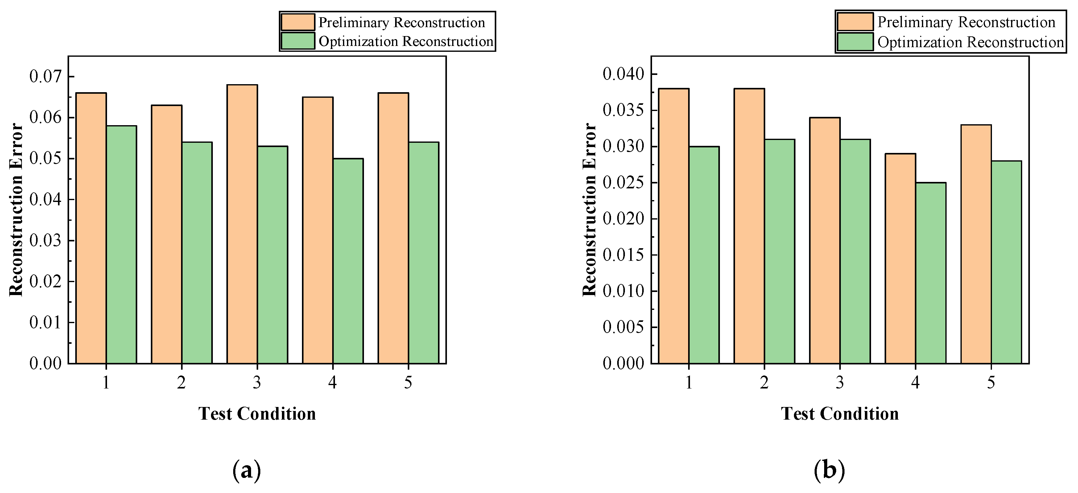
5. Optimization Effect Analysis

The optimized reconstruction algorithm is used to analyze the temperature field, and the influence of the number and arrangement of sensors on the reconstruction accuracy is explored. The number of measuring points is determined to be 13, and the optimal arrangement of measuring points is calculated. The core tensor with dimensions of 9 × 4 × 5 × 13 is applied to build the temperature field of five test cycles, and the overall optimization effect is analyzed. The reconstructed results of the five test conditions after optimization are as follows.

From Figure 10, we can see that the optimized Tucker decomposition algorithm can improve the accuracy of the temperature field reconstruction. The five test conditions are increased by 4.2%, 2.7%, 6.1%, 5.9%, and 6%, respectively.

Test case 5 has the largest average reconstruction error; therefore, 10 measuring points are randomly selected to compare the reconstruction temperature value with the actual temperature value, as shown in Figure 11.

As can be seen from Figure 11, the temperature value reconstructed by the optimization algorithm is basically consistent with the actual temperature value. The error value of the measuring point position 10 is the largest, and the maximum error is 44 K.

To make the application scenarios of the algorithm closer to the actual situation and test the effect of the algorithm in the presence of measurement errors, Gaussian random noise is added. The concept of Signal Noise Ratio (SNR) in the signal processing is introduced to characterize the noise intensity. The temperature measurement signal-to-noise ratio calculation formula used in this paper is as follows.

$$\mathrm{SNR}=10\ln \left(\frac{T}{T_{er}}\right),$$

(12)

where SNR is signal-to-noise(dB); T is actual temperature; T_er is temperature measurement error.

Add noise to the temperature measurement (SNR = 20 dB,30 dB), and for the purpose of for reducing the impact of noise randomness on the reconstruction results, a more general conclusion is obtained. The unoptimized algorithm and the layout of the measuring points calculated based on the optimal layout algorithm are used to reconstruct 1000 times, respectively. The average value of the reconstruction error is obtained as the performance evaluation index of the final algorithm. The comparison results of test conditions 1~5 are shown in Figure 12.

As shown in Figure 10, Figure 11 and Figure 12, after optimizing, the accuracy of the reconstruction is improved obviously. Additionally, in the presence of measurement errors, the optimization effect maintains good consistency.

6. Conclusions

A stable and accurate optimization algorithm for empirical datasets with missing data based on Tucker decomposition has been developed, which realizes the reconstruction of three-dimensional temperature distribution under different working conditions and flame deflection. In the case of missing or distorted empirical data, using the proposed distribution reconstruction algorithm based on Tucker decomposition can repair the missing dataset and complete the reconstruction of temperature distribution. In order to verify the feasibility of the algorithm, different proportions of missing data are repaired and the temperature distribution of five groups of test conditions is reconstructed. The reconstruction error is less than 1%, and a good reconstruction effect is obtained. In the research process, the missing position of the original dataset and the position of the measuring point in the reconstruction process have a great influence on the reconstruction error, indicating that the information carried by different measuring point positions is different in the temperature distribution reconstruction algorithm. Therefore, optimizing the arrangement of measuring points has a significant effect on improving the accuracy of reconstruction results. Using the minimum condition number, the greedy algorithm and the hill-climbing algorithm can improve the reconstruction accuracy by about 4%. At the same time, different degrees of noise are added in the process of temperature reconstruction with errors less than 6.0%, which shows that the algorithm has strong robustness and anti-noise ability. The results show that the Tucker decomposition method is not only suitable for the reconstruction of the temperature distribution of complete datasets, but also for the reconstruction of the temperature distribution of historical missing datasets. This research work on the reconstruction of temperature distribution under the condition of missing empirical data broadens the application range of the reconstruction algorithm and provides a new solution to the problem of data loss and data distortion in industrial measurement.

References

1. Yang, W.; Xue, B.; Wang, C. Image Super Resolution Reconstruction Based MCA and PCA Dimension Reduction. Adv. Mol. Imaging 2018, 8, 82144. [Google Scholar] [CrossRef] [Green Version]
2. Tucker, L.R. Implications of factor analysis of three-way matrices for measurement of change. Probl. Meas. Chang. 1963, 15, 122–137. [Google Scholar]
3. Maldonado-Chan, M.; Mendez-Vazquez, A.; Guardado-Medina, R.O. Multimodal tucker decomposition for gated rbm inference. Appl. Sci. 2021, 11, 7397. [Google Scholar] [CrossRef]
4. Li, R.; Pan, Z.; Wang, Y.; Wang, P. The correlation-based tucker decomposition for hyperspectral image compression. Neurocomputing 2021, 419, 357–370. [Google Scholar] [CrossRef]
5. Marmoret, A.; Cohen, J.E.; Bertin, N.; Bimbot, F. Uncovering audio patterns in music with Nonnegative Tucker Decomposition for structural segmentation. arXiv 2021, arXiv:2104.08580. [Google Scholar]
6. Karami, A.; Yazdi, M.; Asli, A.Z. Noise Reduction of Hyperspectral Images Using Kernel Non-Negative Tucker Decomposition. IEEE J. Sel. Top. Signal Process. 2011, 5, 487–493. [Google Scholar] [CrossRef]
7. Zhang, J.; Han, Y.; Jiang, J. Tucker decomposition-based tensor learning for human action recognition. Multimedia Syst. 2015, 22, 343–353. [Google Scholar] [CrossRef]
8. Zhao, M.; Li, W.; Li, L.; Ma, P.; Cai, Z.; Tao, R. Three-Order Tensor Creation and Tucker Decomposition for Infrared Small-Target Detection. IEEE Trans. Geosci. Remote Sens. 2021, 60, 5900511. [Google Scholar] [CrossRef]
9. Liu, Z.; Liu, S.; Chen, M.; Zhang, Y.; Yao, P. Application of Tucker Decomposition in Temperature Distribution Reconstruction. Appl. Sci. 2022, 12, 2749. [Google Scholar] [CrossRef]
10. Qin, L.; Liu, S.; Kang, Y.; Yan, S.A.; Schlaberg, H.I.; Wang, Z. Wind velocity distribution reconstruction using CFD database with Tucker decomposition and sensor measurement. Energy 2018, 167, 1236–1250. [Google Scholar] [CrossRef] [Green Version]
11. Hou, Z.; Li, W.; Tao, R.; Du, Q. Three-Order Tucker Decomposition and Reconstruction Detector for Unsupervised Hyperspectral Change Detection. IEEE J. Sel. Top. Appl. Earth Obs. Remote Sens. 2021, 14, 6194–6205. [Google Scholar] [CrossRef]
12. Zhang, Q.; Wang, H.; Plemmons, R.J. Tensor methods for hyperspectral data analysis: A space object material identification study. J. Opt. Soc. Am. A 2008, 25, 3001–3012. [Google Scholar] [CrossRef] [PubMed]
13. Everson, R.; Sirovich, L. Karhunen-Loeve procedure for gappy data. J. Opt. Soc. Am. A Opt. Image Sci. Vis. 1995, 12, 1657–1664. [Google Scholar] [CrossRef] [Green Version]
14. Zhang, X. Matrix Analysis and Application; Tsinghua University Press: Beijing, China, 2013; pp. 453–471. [Google Scholar]
15. Polansky, J.; Wang, M. Proper Orthogonal Decomposition as a technique for identifying two-phase flow pattern based on electrical impedance tomography. Flow Meas. Instrum. 2017, 53, 126–132. [Google Scholar] [CrossRef] [Green Version]
16. Tsamardinos, I.; Brown, L.E.; Aliferis, C.F. The max-min hill-climbing Bayesian network structure learning algorithm. Mach. Learn. 2006, 65, 31–78. [Google Scholar] [CrossRef]
Figure 1. Flow diagram of prior dataset completion.
Applsci 12 10814 g001
Figure 2. Bimodal temperature field model in the computational domain at z = 1.5 m: (a) a = 1200, b = 1200, c = 1.0, d = 3.0; (b) a = 1700, b = 900, c = 2.0, d = 3.0.
Applsci 12 10814 g002aApplsci 12 10814 g002b
Figure 3. 1000 reconstruction errors of condition 5.
Applsci 12 10814 g003
Figure 4. Bimodal temperature distribution model in the computational domain: (a) calculation results; (b) reconstruction results.
Applsci 12 10814 g004
Figure 5. Reconstruction errors of bimodal temperature distribution model.
Applsci 12 10814 g005
Figure 6. Reconstruction errors of different missing ratios.
Applsci 12 10814 g006
Figure 7. Optimized effects of core tensor dimension.
Applsci 12 10814 g007
Figure 8. Comparison of reconstruction results with different sensor numbers (10–25).
Applsci 12 10814 g008
Figure 9. Comparison of Optimized Effects.
Applsci 12 10814 g009
Figure 10. Optimized Effects of Reconstruction Algorithm.
Applsci 12 10814 g010
Figure 11. Comparison between Reconstructed Temperature and Actual Temperature of 10 points.
Applsci 12 10814 g011
Figure 12. Optimized Effects of Reconstruction Algorithm with Noise: (a) SNR = 20; (b) SNR = 30.
Applsci 12 10814 g012