Article

Towards Reliable Baselines for Document-Level Sentiment Analysis in the Czech and Slovak Languages

Institute of Informatics, Slovak Academy of Sciences, 84507 Bratislava, Slovakia
*
Author to whom correspondence should be addressed.
Future Internet 2022, 14(10), 300; https://doi.org/10.3390/fi14100300
Submission received: 26 September 2022 / Revised: 8 October 2022 / Accepted: 17 October 2022 / Published: 19 October 2022
(This article belongs to the Special Issue Trends of Data Science and Knowledge Discovery)

Abstract

:
This article helps establish reliable baselines for document-level sentiment analysis in highly inflected languages like Czech and Slovak. We revisit an earlier study representing the first comprehensive formulation of such baselines in Czech and show that some of its reported results need to be significantly revised. More specifically, we show that its online product review dataset contained more than 18% of non-trivial duplicates, which incorrectly inflated its macro F1-measure results by more than 19 percentage points. We also establish that part-of-speech-related features have no damaging effect on machine learning algorithms (contrary to the claim made in the study) and rehabilitate the Chi-squared metric for feature selection as being on par with the best performing metrics such as Information Gain. We demonstrate that in feature selection experiments with Information Gain and Chi-squared metrics, the top 10% of ranked unigram and bigram features suffice for the best results regarding online product and movie reviews, while the top 5% of ranked unigram and bigram features are optimal for the Facebook dataset. Finally, we reiterate an important but often ignored warning by George Forman and Martin Scholz that different possible ways of averaging the F1-measure in cross-validation studies of highly unbalanced datasets can lead to results differing by more than 10 percentage points. This can invalidate the comparisons of F1-measure results across different studies if incompatible ways of averaging F1 are used.

Graphical Abstract

1. Introduction

Sentiment analysis (also known as opinion mining) is one of the most dynamically growing areas of natural language processing (NLP). It goes back to the early 2000s, when a handful of fundamental studies like Pang et al. [1], Turney [2], Turney and Littman [3], and Dave et al. [4] laid foundations for its subsequent explosive growth, fueled primarily by the availability of large quantities of opinionated online texts in English, mostly user-rated reviews of movies, products and services [5]. Drawing mainly on Bing Liu’s excellent “in-depth introduction” [6] and his recent exhaustive textbook [7], as well as on selected comprehensive reviews [5,8,9], we briefly summarize here its most salient aspects.

1.1. Terminology

The first thing that needs clarification is terminology. Although the name of the field has by now largely converged towards two nearly synonymous alternatives, sentiment analysis and opinion mining (or their concatenation), the fact remains that it has to deal with a host of closely interrelated, but not completely identical, manifestations of human subjectivity in a textual form, such as opinions, sentiments, evaluations, appraisals, attitudes, and emotions. These can be directed towards various entities, such as products, services, organizations, individuals, issues, events, topics, or even their attributes. In this respect, we might say that subjective texts express personal feelings, views or beliefs, while objective ones simply state (in principle) verifiable external facts.
Sometimes, all the diverse forms of subjectivity are lumped together and designated indiscriminately as “opinions” or “sentiments”, although conferring such a wide meaning to these two terms might easily breed confusion. We therefore side with those who propose to use both only for the forms of subjectivity that express or imply positive or negative feelings or attitudes towards something or somebody, and we follow Liu [6,7] in calling such documents and sentences opinionated. It may not be immediately obvious, but there are emotions (e.g., moods, such as melancholy) that are not directed at any particular object—at least not on the surface—while the directedness of others, e.g., that of surprise, does not easily fit into the categories of positive and negative (albeit the context may occasionally impart to it either hue). To avoid a long detour into a potentially controversial issue of how many basic emotions there are, we restrict ourselves to merely echoing the observation of Tsytsarau and Palpanas [10] that most authors in NLP seem to prefer the scheme with six basic emotions (anger, disgust, fear, joy, sadness, surprise) originally proposed by Ekman et al. [11].
From the preceding terminological clarifications, it might seem that opinionated texts should always be a subset of subjective ones, but the reality is more complex: opinions and sentiments may be implied indirectly, contextually, without any explicit indicators of subjectivity in the text. One example could be the sentence, “I bought this car and after two weeks it stopped working.” Here, a negative opinion is conveyed by an objective fact, whose undesirability is clear only to those who share implicit general expectations regarding cars. (A complementary example of a subjective sentence that is nevertheless not opinionated could be “I think he went home after lunch.” [7]) Moreover, as Pang and Lee [8] pointed out, the distinction between what is objective and what is subjective can be rather subtle: is “long battery life” or “a lot of gas” really objective? And how about the difference between “the battery lasts 12 h” and “the battery only lasts 12 h”? Consequently, and despite its deceptively simple appearance, sentiment analysis turns out to be a very difficult task. It is from this perspective that we can appreciate the depth of its pithy informal definition as “a field of study that aims to extract opinions and sentiments from natural language text using computational methods” [7].

1.2. Challenges

Apparently, the most straightforward way to identify opinionated texts is through the presence of sentiment words, also called opinion words. These consist mainly of adjectives and adverbs (good, bad, well, poorly, etc.), but also some nouns, verbs, phrases and idioms (disaster, to fail, to cost someone an arm and a leg, etc.). However, as Liu [6] notes, sentiment lexicons (lists of sentiment words along with their positive or negative polarities) cannot be a panacea. One reason is that certain sentiment words may acquire opposite orientations in different contexts. For example, Turney [2] observes that the word “unpredictable” could be positive regarding a movie plot but negative regarding a car’s steering capabilities, while Pang and Lee [8] mention the phrase “Go read the book,” which might convey a positive sentiment in a book review but a negative one in a movie review. Moreover, as Fahrni and Klenner [12] point out, this polarity flip can happen even within one domain—compare for instance the polarity of the word “cold” in “cold beer” with that in “cold pizza”.
Another reason limiting the utility of sentiment lexicons is that some sentences containing sentiment words may not express any sentiment at all—typically questions and conditionals, for example, “Can you tell me which Sony camera is good?” or “If I can find a good camera in the shop, I will buy it”. This, however, is not universal; for example, the question “Does anyone know how to repair this terrible printer?” clearly carries a negative attitude toward the printer [7]. Then there are sarcastic sentences, which actually mean the opposite of what they appear to say on the surface, as well as seemingly objective sentences without any sentiment words, but which nevertheless carry an evaluative attitude such as the one about the new car that broke down after two weeks.
Pang and Lee [13] also mention a few other issues affecting sentiment analysis, especially when both fine-grained ratings (e.g., stars) and evaluative texts (reviews) are assigned to opinion targets. These problems include:
(a)
Individual reviewer inconsistency, e.g., when the same reviewer associates their own very similarly worded reviews with different star ratings;
(b)
Lack of inter-reviewer calibration, e.g., high praise by an understated author can be interpreted as a lukewarm or neutral reaction by others;
(c)
Ratings not entirely supported by the review text, as when the review mentions only some partial aspects or details, while the rating captures the overall impression of the target, including aspects not explicitly mentioned in the text.
As a result, there is considerable uncertainty inherent in the very nature of sentiment analysis, which even the human mind cannot entirely overcome. Human interrater agreement studies can therefore be taken as providing upper bounds on the accuracy that can be reasonably expected of automated sentiment analysis methods. It turns out that human interrater agreement can be surprisingly low, especially for fine-grained sentiments, as Hazarika et al. [14] observed. Studying consistency of human ratings of Apple iTunes applications on the scale from one to four stars, the exact interrater agreement among their three human raters was below 41%. To account for subtle variations in human interpretation, they proposed to consider human ratings to be in agreement if they varied by at most one level of rating. This “adjacent interrater agreement” then approached 89.5%, which showed that after all, the three raters could still be considered fairly consistent. In a similar context, Batista et al. [15] report the levels of exact interrater agreement between two human judges distinguishing three levels of sentiment (positive, neutral, negative) to vary between 79% and 90%. It is important to be aware of these limits when forming expectations or evaluating the performance of automated methods.

1.3. Approaches

In general, sentiment analysis can be carried out on the level of documents, sentences, or entities mentioned in the text and their aspects. Document-level is properly applicable only to documents which evaluate a single entity, such as product or movie reviews. Because we deal precisely with such documents in this article, from now on we will concentrate primarily on document-level sentiment analysis.
Tsytsarau and Palpanas [10] broadly categorized document-level sentiment analysis approaches into four types: dictionary-based, statistical, semantic, and machine learning-based. In principle, each of these can be conceived either as a classification task, labelling documents as “positive”, “negative”, “neutral”, etc., or as a regression task, trying to predict some sort of numeric or ordinal sentiment score for each document, e.g., on a scale from one to five stars.
Of these, the most straightforward is the dictionary approach, which exploits pre-built sentiment lexicons and dictionaries, such as General Inquirer [16], WordNet-Affect [17], SentiWordNet [18], or Emotion lexicon [19]. In the dictionary approach, the polarity of a text is usually computed as a weighted average of the lexicon-provided polarities of its sentiment words, accounting also for their modifiers (negation, intensification, etc.). The weights used in this calculation may be static or computed dynamically, reflecting, e.g., the distance of a given sentiment word from the closest topic word [10]. It is also possible to evaluate the polarity of a text based on the polarity of its longer n-grams, as in [20]. In general, however, relying on universal polarity values from lexicons was shown to be unreliable, since sentiment words can change their polarity in different contexts, and sometimes even within the same context. This motivated the development of more advanced forms of sentiment analysis.
The statistical approach aims to overcome such problems by constructing corpus-dependent sentiment lexicons. It is based on the observation that similar opinion words frequently appear together in a corpus. Conversely, if two words frequently appear together within the same context, they are likely to share the same polarity. Therefore, the polarity of an unknown word can be determined by calculating the relative frequency of its co-occurrence with another word, which invariantly preserves its polarity (a prototypical example of such a “reference” word is “good”). This fact motivated Peter Turney [2,3] to exploit the pointwise mutual information (PMI) criterion originally proposed by Church and Hanks [21], and derive from it the sentiment polarity of a word as the difference between its PMI values relative to two opposing lists of words: positive words, such as “good, excellent”, and negative words, such as “bad, poor”.
The semantic approach is akin to the statistical one in that it directly calculates sentiment polarity values for words (thus bypassing the need for external sentiment lexicons) except that it computes the similarity between words differently. Its defining principle is that semantically close words should receive similar sentiment polarity values. As with statistical methods, two sets of seed words with positive and negative sentiments are used as a starting point for bootstrapping the construction of a dictionary. This initial set is then iteratively expanded with their synonyms and antonyms, drawn from a suitable semantic dictionary such as WordNet [22,23]. The sentiment polarity for an unknown word can be determined by the relative count of its positive and negative synonyms, or it may simply be discarded. Alternatively, Kamps et al. [24] used the relative shortest path distance of the “synonym” relation. In any case, it is important to account for the fact that the synonym’s relevance decreases with its distance from the original word, so the same principle should be applied to assigning the polarity value to the original word.
The above three approaches were especially prominent in the early days of sentiment analysis; later they were mostly eclipsed by classical machine learning or incorporated into it as special forms of data pre-processing, feature construction and feature selection. Some of them could even be considered forms of machine learning in their own right. Thus, for example, Peter Turney [2] called his early work (considered to be of “statistical” nature by Tsytsarau and Palpanas [10]), “unsupervised classification”, a somewhat paradoxical but still legitimate term employed also by Liu [7].
In classical machine learning (ML), a model is learned in a supervised or unsupervised way from a training corpus, and then used to classify new, previously unseen texts. Its key success factors are the choice of the learning algorithm, the quality and quantity of the training data, and the quality of feature engineering and feature selection, which may require considerable domain expertise.
In many applications, binary features (recording just the presence or absence of a certain feature in a given text) perform remarkably well. In others, capturing relative frequency of each feature might yield better results. Moreover, as Osherenko and André [25] observed, in most cases the features may be reduced to a small subset of the most affective words without any significant degradation of the model’s performance. The same authors also noted that (at least for their corpus) word frequencies contained approximately the same amount of information as sentiment annotations in their sentiment lexicons.
Since sentiment classification is a type of text classification, in principle, any supervised ML method suitable for the latter can also be applied to the former. In practice, Naïve Bayes (NB) and Support Vector Machines (SVM) have been (and still are) very popular in English [26,27], especially for sentiment analysis of short messages like Twitter [28,29]. From the recent work exploiting deep learning techniques we might mention the study of COVID-19 vaccination-related sentiments by Reshi et al. [30], or various attempts to combine deep learning with other techniques such as ensemble learning [31], dual graphs [32], word dependencies [33] or topic modeling and clustering [34,35]. Given the growing demand for trustworthiness, explainability and accountability of AI applications, the use of explainable AI techniques in sentiment analysis is also growing [36,37]. Of course, many more algorithms and their variations than we could possibly list here have been tried by various researchers—for a detailed overview we recommend the latest book by Liu [7] or one of the recent comprehensive reviews, such as [38,39].
While NLP in general, and sentiment analysis in particular, receive a lot of research attention and funding in English (and possibly in a few other major languages), smaller languages are largely left behind. Their uneven progress has been vividly documented in a series of white papers produced by the European META alliance (http://www.meta-net.eu/whitepapers/overview (accessed on 17 October 2022)). Their Key Results section (http://www.meta-net.eu/whitepapers/key-results-and-cross-language-comparison (accessed on 17 October 2022)) shows English to be the only language with “good support” across all the four major NLP dimensions (Text Analysis, Speech Processing, Machine Translation, Resources), with French and Spanish coming next and enjoying consistently “moderate support” across them. Dutch, German and Italian enjoy fragmentary support in Machine Translation and a moderate one in the remaining three categories, while most of the remaining European languages enjoy only fragmentary or no support.
This explains why the latest deep learning techniques and trends, already prominent in English, such as Bidirectional Encoder Representations from Transformers (BERT) [40] and its derivatives, e.g., RoBERTa (A Robustly Optimized BERT Pretraining Approach) [41], have only recently started to appear in smaller languages such as Czech and Slovak [42,43,44,45]. Although they promise to revolutionize the whole field of NLP, to objectively measure the progress and the advantages that they bring, reliable baselines must first be established on the basis of methods that historically preceded them. That is precisely the goal and the main contribution of our present work. Moreover, related contemporary research in NLP shows that these new deep learning techniques will not simply render classical machine learning obsolete, but rather turn it into a valuable auxiliary tool to be used whenever their results or their operation need to be investigated from the perspective of robustness, adequacy, quality, accountability or explanation. Examples of techniques that can thus utilize classical machine learning include, for instance, “diagnostic classifiers” [46], “probing tasks” [47], and “structural probes” [48,49]. It will therefore continue to pay off for researchers of artificial intelligence to remain well-versed in classical machine learning techniques too.
The rest of this article is structured as follows: In Section 2 we review the related work in the Czech and Slovak languages. In Section 3 we summarize the relevant experiments and results by Habernal et al. [50], some of which we then choose for replication. Section 4 describes our replication experiments and their results, while Section 5 discusses their implications and adds some relevant methodological advice toward increased replicability and reliability of sentiment analysis results in general. Finally, Section 6 concludes our work with a short summary and an outline of future work.

2. Related Work

In this section we concern ourselves only with sentiment analysis in Czech and Slovak. An extensive treatment of sentiment analysis in Czech is provided in the comprehensive monograph by Veselovská [51]. A shorter, but still very useful and readable introduction can be found in Klimešová [52]. Since both are freely available online, we shall only sketch a brief overview of the field here, focusing mainly on areas of relevance to our present work.
Soon after the explosion of interest in sentiment analysis in English in the early 2000s, initial visions were formulated and subsequent attempts made to leverage or transfer its techniques to other languages as well, often relying on existing parallel corpuses and various general NLP approaches such as machine translation. Examples in Czech include, e.g., [53,54,55]. Since around 2010 several authors, e.g., Veselovská et al. [56] and Červenec [57], undertook the creation of manually tagged datasets specifically for the purposes of sentiment analysis in Czech. With some justification it could be claimed that this line of work reached its acme in the work of Habernal et al. [50], an extended version of their earlier conference paper [58], which represents the first systematic and in-depth evaluation of data pre-processing and classical machine learning methods for sentiment analysis of Czech social media. The authors first collected and made public three datasets (Facebook posts, movie reviews and product reviews; all freely available at http://liks.fav.zcu.cz/sentiment/ (accessed on 17 October 2022)), outstripping earlier such efforts by an order of magnitude, and then used them to evaluate the utility of several data pre-processing techniques, different types of features and feature selection methods to sentiment analysis in Czech. To the best of our knowledge, this study is still unrivalled in its breadth and the level of detail with which it covered the field as it existed at that point in time. Its results (which we describe in more detail in Section 3) established a kind of informal baseline against which subsequent attempts at further improvement could be (and often were) evaluated. These subsequent attempts proceeded along various directions, from engineering new types of features [59], to considering wider context beyond the individual review being analyzed [60,61]. Not long afterwards, initial attempts to apply neural networks to sentiment analysis in Czech appeared, such as Lenc and Hercig [62], Hercig et al. [63] or Libovický et al. [64]. Somewhat surprisingly, in no case were the employed neural architectures able to significantly outperform the established classical supervised ML models, such as Maximum Entropy. Moreover, a later attempt by Cano and Bojar [65] to apply an even deeper neural network failed due to overfitting, indicating that the restricted size of available training corpuses for sentiment analysis in Czech did not permit truly deep neural networks to utilize their full potential. Consequently, classical supervised machine learning remained a legitimate part of the state of the art in sentiment analysis in Czech until around 2020, when first Czech variants of BERT and RoBERTa models [42,43,44] eventually broke the impasse and established themselves as the new “state of the art”. These new models are universal and rely on truly deep neural architectures pre-trained in an unsupervised manner on much larger Czech corpuses, typically obtained from the web without any need for manual or semi-automatic annotation and tagging. These models can then be adapted for sentiment analysis by additional fine-tuning with the help of much smaller training sets, such as the manually annotated ones currently available for sentiment analysis in Czech.
Slovak language, historically younger and restricted to a smaller population than Czech, exhibits a similar developmental pattern: Krchnavy and Simko [66] created the first corpus of 1588 Slovak Facebook posts, relatively evenly assigned by human annotators into five classes, from strongly positive to strongly negative. The authors then used it to evaluate four most popular approaches to sentiment analysis (Naïve Bayes, Maximum Entropy, Support Vector Machines, and Lexicon-based) in combination with various data pre-processing steps (with or without emoticon normalization, diacritics reconstruction, lemmatization, and negation handling). Unlike Habernal et al. [50], however, they only used word unigrams as features, i.e., the bag of words representation of each Facebook post. Despite this limitation, they too observed that Maximum Entropy algorithm performed best, and that the envisaged data pre-processing steps were indeed important. (A somewhat puzzling exception was the damaging effect of their attempt at proper negation handling on all the tested approaches except the lexicon-based one.) One year later, Pecar, Simko and Bielikova [67] used a real-life dataset consisting of 5318 Slovak reviews of various services assigned into seven categories, from most negative (−3) to most positive (3), in order to compare the accuracy of a deep neural network against a baseline SVM model. Here again, as in earlier such attempts in Czech, the results were ambiguous: although their best deep learning model (code-named M2) slightly outperformed the best SVM model in fine-grained sentiment classification into seven classes (by about 0.22 of a percentage point), it lagged by more than two percentage points behind SVM in classification into three classes (positive, negative, neutral). In their subsequent work [68], the same authors achieved further significant improvement of more than six percentage points in accuracy on the same dataset by a combination of deep contextualized word representations based on pre-trained version of Embeddings from Language Models (ELMo) for Slovak language with Bi-LSTM (Bi-Directional Long Short-Term Memory) and attention mechanism. Recently, the SlovakBERT model with RoBERTa architecture [45] heralded the arrival of the new state of the art in Slovak, demonstrating further modest improvements even over the model based on Bi-LSTM with ELMo and attention mechanism.
To be able to objectively judge the extent to which these new techniques outstrip the past ones, we need to revisit the earlier classical machine learning experiments representing the historical “baseline” and rectify some of their apparently erroneous claims and reported results. As part of this effort, we provide here the following main contributions to sentiment analysis in the Czech and Slovak languages:
  • We validate and correct the main baseline results for Czech reported by Habernal et al. [50] on their three datasets;
  • We show that their online product review dataset from Mall.cz contains more than 18% of non-trivial duplicates and must therefore be de-duplicated before analysis;
  • We demonstrate that, without deduplication, the macro F1-measure results for the Mall.cz dataset are inflated by more than 19 percentage points and thus completely unreliable;
  • We establish that part-of-speech-related features have no damaging effect on machine learning algorithms, contrary to the claim made by Habernal et al. [50];
  • We rehabilitate the Chi-squared metric for feature selection as being on par with the best performing metrics like Information Gain;
  • We demonstrate that in feature selection experiments with Information Gain and Chi-squared metrics, the top 10% of ranked unigram and bigram features suffice for the best results regarding the online product and movie reviews, while the top 5% of ranked unigram and bigram features are optimal for the Facebook dataset;
  • We reiterate an important, but often ignored, warning by Forman and Scholz [69] that different possible ways of averaging the F1-measure in cross-validation studies of highly unbalanced datasets can lead to results differing by more than 10 percentage points. This can invalidate comparisons of F1 results across different studies if incompatible ways of averaging F1 are used.

3. Summary of Relevant Experiments and Results Reported in [50]

Habernal et al. [50] first created an entirely new Facebook dataset consisting of around 10,000 Czech posts, which they manually assigned into three main classes, positive, negative, and neutral. (There was also a small “bipolar” class, which was excluded from further experiments.) The authors also compiled two additional datasets, one consisting of 91,381 movie reviews from the Czech–Slovak Movie Database csfd.cz, the other consisting of 145,307 product reviews from a large Czech e-shop Mall.cz. Since reviews from these two additional sources were accompanied by star ratings, these were used for assigning the reviews into three classes: positive, negative, and neutral. We show selected examples from these three datasets in Table 1.
Habernal et al. [50] then used these three datasets to evaluate the utility of various combinations of data pre-processing techniques, types of features and feature selection methods for sentiment analysis in Czech (see Table 2 for a summary of their considered methods and approaches). In their experiments, they relied on Maximum Entropy (MaxEnt) and Support Vector Machines (SVM) as the two most promising algorithms identified in the published literature. For each dataset, they performed both a binary classification into the “positive” and “negative” classes, and a ternary classification, which also included the “neutral” class. In most cases, the Maximum Entropy algorithm outperformed the SVM. In the results reported below, we focus only on ternary classification with the Maximum Entropy algorithm, which was directly relevant to our own research work.
Since some of the pre-processing techniques are mutually exclusive (e.g., stemming and lemmatization), Habernal et al. [50] only evaluated their meaningful combinations. Moreover, all their pre-processing pipelines used tokenizing, part-of-speech (POS) Tagging, and stopword removal, and were thus distinguished by the presence or absence of the remaining pre-processing steps. (It also turned out that Named Entity Filtering never helped, so the “winning” pipelines never used it.) All the resulting data pre-processing pipelines were then combined with various feature types to determine the optimum configuration for each of the three datasets (see Section 3.1 for the results). Habernal et al. [50] additionally applied various feature selection methods to selected configurations to see if they could further improve the macro-F1 measure by pruning useless attributes (see Section 3.2).

3.1. Results for Optimum Configurations Using All Features of the Included Feature Types

Facebook dataset: In the ternary classification into positive, negative, and neutral classes, the “collective winners” were the preprocessing pipelines that avoided phonetic transcription and lemmatization. In combination with all the available feature types, such configurations systematically achieved the macro-F1 score of 69%. Somewhat surprisingly, the same result was achieved by two specific pre-processing pipelines based on High Precision Stemmer (HPS) with either lower-casing or phonetic transcription even with a reduced feature set comprising just word unigrams, bigrams and POS-related features.
Product review dataset (Mall.cz): In the ternary classification, there were four configurations that managed to cross the 75% level of the macro-F1 measure. The best one (75.30%) was based on Lemmatization by OpenOffice, and the next two on light stemming. Quite surprisingly, all the four achieved this remarkable feat just on the basis of word unigrams and bigrams. In fact, adding the POS-related features into the mix seemed to cause a “catastrophic” drop of about 15–20 percentage points in the macro-F1 across the board. This was one of the things that caught our attention as deserving a dedicated replication experiment (which we describe in more detail in Section 4) because other researchers using POS-related features, such as [70,71], did not report any such adverse effects.
Movie review dataset (csfd.cz): In the ternary classification, there were six configurations that crossed the level of 78% in the macro-F1 score, and all of them used some form of stemming. The best configuration (HPS stemming with phonetic transcription) reached the macro-F1 of 78.50%. As with the product reviews, they all managed to do so just on the basis of word unigrams and bigrams, whereas adding the POS-related features again seemed to lead to a drop in the macro-F1 across the board, although this time only by 5 to 10 percentage points.

3.2. Feature Selection Experiments

Habernal et al. [50] performed the feature selection experiments only in the context of ternary classification in the hope of increasing its macro-F1 measure by pruning useless input attributes. In each of these experiments, 10% of the training set was set apart as held-out data on which an optimal feature weight cut-off threshold value was to be determined for each feature selection metric. If successful, this procedure would find a local maximum of the macro-F1 measure, ideally achieved with the help of only a fraction of (the most important) input attributes. However, despite repeating this experiment in dozens of different configurations, only in a single case was a statistically significant (but actually very modest) improvement of 0.47 percentage point achieved. (That unique case was the Mutual Information metric applied to the product reviews represented by word unigrams and bigrams, which was pre-processed by the HPS Stemming and lowercasing pipeline.) For illustration purposes, the authors provided a number of dependency graphs of the macro-F1 measure on the feature weight cut-off threshold value for each feature selection metric. In these figures, the Chi-squared metric appeared to behave strikingly differently from the other metrics—another anomaly that caught our attention because in our own previous work [72,73] we saw the Chi-squared metric to perform very well, on par with the Information Gain. We therefore considered it worthy of a dedicated replication experiment, which we describe in the next section.

4. Replication Experiments and Their Results

When we first came across the work of Habernal et al. [50], our intention was to use it as a baseline which we would try to improve upon. At that time, we were trying to collect our own dataset of online product reviews in Slovak, and because of the similarity of Slovak to Czech, we expected that we would be able to match Habernal at al.’s [50] macro-F1 results for online product reviews quite easily with our selection of machine learning algorithms and Slovak data. Unfortunately, however hard we tried our results kept lagging behind theirs by more than ten percentage points. Ultimately, we were forced to accept the fact that to solve this mystery we would need to replicate Habernal et al.’s [50] experiments on their datasets, using both our and their algorithms, and thoroughly analyze any significant differences in the results. It turned out that with their datasets, our algorithms gave comparable results to theirs. In this way, the mystery was narrowed down to the difference between the two datasets: why should a dataset of Slovak online product reviews be so much more difficult for machine learning than the Czech one? Slovak and Czech are so close that their minor differences did not seem to be a plausible explanation at all. Finally, after a long and tiring investigation of various alternatives, our lead author (J.M.) came up with a surprising answer: because the Czech product review dataset from Mall.cz contained a lot of duplicate records! Of course, it is quite conceivable that different customers may use the same short judgement like “excellent product” repeatedly for different products, but it is very unlikely that longer reviews could be thus reproduced in significant quantities accidentally. Long duplicates are therefore much more likely to be the result of either a deliberate spamming or an inadvertent duplication during the data collection process. In what follows, we therefore focus only on such “nontrivial” reviews, which we empirically define as being longer than 10 words.
To illustrate the extent of duplication among nontrivial product reviews from Mall.cz, here are some summary statistics: more than 17,500 distinct nontrivial reviews exist in two or more copies (out of which, more than 6700 have three or more copies, and more than 1800 have four or more copies). Overall, more than 18% of records in the Mall.cz product review dataset consist of such non-trivial duplicates. In Table 3, Table 4 and Table 5 we provide more-detailed information of duplicates per class (positive, negative, and neutral). These tables also reveal the absolute record-holders: there is one nontrivial negative review of which 27 verbatim copies exist in the dataset, and one positive review with 20 verbatim copies. (By way of example, searching for the string “vyzkouzšeno týden v Roháčích” (sic) should help identify nine verbatim copies of that particular review in the positive class of this dataset.) As far as we could see, these duplicates did not seem to exist on the Mall.cz webpage, so they appear to be an artefact of a faulty data collection process. Duplicates inflate the macro-F1 measure because random selection tends to make copies of the same review to be simultaneously present in both the training set and the test set. Interestingly, this issue significantly affected only the product reviews from Mall.cz, not the other two datasets. Although there were a few duplicates in each of them, their numbers, as well as their effect on the achieved macro-F1 measure, were minimal. The discovery of this problem emboldened us to look more inquisitively on other unexpected or otherwise anomalous results and claims in the article and test their validity as well. Overall, our replication experiments in this section cover the following issues:
  • What are the true baseline macro-F1 results for the three datasets after deduplication?
  • Is the alleged damaging effect of the POS-related features on product reviews real?
  • Is the Chi-Squared metric really so detrimental to feature extraction and so different from other metrics?
We first performed these replication experiments on the original datasets with duplicates so that our results were directly comparable to those reported in Habernal et al. [50]. We then repeated the experiments on de-duplicated versions of the datasets in order to evaluate the difference. (Please note that we only de-duplicated “nontrivial” reviews longer than10 words, giving the benefit of doubt to shorter duplicates.) Given our focus on product reviews, we first tried the data pre-processing pipeline termed “Lo” in [50] because it ranked among the best for product reviews (see Table 6, last row in [50]). Eventually, however, we opted for “ShCl” pipeline because it seemed to give us slightly better overall results. This “ShCl” pipeline consists of stemming with HPS stemmer on top of mandatory tokenization, POS tagging, and stop-word removal.
Table 3. Statistical distribution of the number of verbatim copies among nontrivial positive product reviews from Mall.cz.
Positive Product Reviews (Mall.cz)
Number of copies2015121110987654321
Number of distinct
reviews
1122281523552168543427712626,101
Table 4. Statistical distribution of the number of verbatim copies among nontrivial negative product reviews from Mall.cz.
Negative Product Reviews (Mall.cz)
Number of copies2787654321
Number of distinct reviews113122312039610724486
Table 5. Statistical distribution of the number of verbatim copies among nontrivial neutral product reviews from Mall.cz.
Neutral Product Reviews (Mall.cz)
Number of copies10987654321
Number of distinct reviews2191139783561097262312,007
Table 6. Macro-F1 results of our replication experiments compared with those of Habernal et al. [50] for classification into three classes by the Maximum Entropy algorithm.
Macro-F1 Results Category:Facebook (%)Product Reviews Mall.cz (%)Movie Reviews csfd.cz (%)
Best result in [50] regardless of configuration6975.3078.50
Result in [50] for “ShCl” configuration using all word unigrams and bigrams6674.0278.21
Our replicated result for “ShCl” configuration using all unigrams and bigrams64.7776.278.9
Our result for “ShCl” configuration using all unigrams and bigrams AFTER DEDUPLICATION66.457.0778.26
Given that we use different tools (Weka, Matlab, Java) than [50], our attempt at reconstructing their operational environment is not perfect, but the differences are minor and could not count as plausible explanations of major discrepancies that we observed in the following replication experiments. As other authors before us, we also need to point out that since no canonical split into folds was provided by the creators of these datasets, we cannot recreate the exact assignment into folds that they used. Different assignments of records into folds can easily cause a difference of several percentage points in the macro-F1 measure. In our replication experiments we therefore focus only on truly massive differences of more than five percentage points between our results and those reported in [50]. Moreover, as we shall see later in Section 5, significant differences between F1 scores can also arise due to different ways of calculating and averaging F1 in the used tools. To minimize such undesirable tool-dependent biases, we invite other researchers to also try and replicate these experiments in the tools and environments that they routinely use. The value of the datasets and systematic exploration of the field provided by [50] is high enough to deserve such continual attention and removal of any significant errors that may have crept into it.

4.1. True Macro-F1 Baselines for the Three Datasets

Table 6 compares the results of our replication experiments with those reported in [50]. The experiments consisted of classification by the Maximum Entropy algorithm into three classes (positive, negative, neutral) using all word unigrams and bigrams without any filtering by feature selection, and they refer to Table 2 and Table 6 provided in [50].
Our Table 6 shows that the results for all the three datasets with duplicates were replicated successfully; the minor differences of up to two percentage points can easily be explained by different assignment of records into folds and, possibly, also by a different implementation of the F1 measure calculation in our tools (which was for us opaque). The most important finding was the massive drop in the macro-F1 measure for the product review dataset Mall.cz after deduplication—by more than 19 percentage points. It may be purely accidental, but this percentage drop seems to be roughly equal to the proportion of duplicates in the dataset. In both the Facebook and the movie review dataset csfd.cz, the proportion of duplicates was negligible and therefore affected their macro-F1 scores only marginally.

4.2. On the Alleged Damaging Effect of POS-Related Features

Habernal et al. [50] report a massive drop in the macro-F1 score after adding the POS-related attributes into the product review dataset from Mall.cz—more precisely, a drop from 74.02% to just 54.88% for the “ShCl” preprocessing pipeline. Given that word unigrams and bigrams together comprise more than 70,000 attributes for this particular dataset, and the POS-related features at most a few dozen, we found it hard to believe that they could have such a strong “poisoning” effect on the macro-F1 metric. In fact, on purely theoretical grounds—because the POS-related features might carry a different kind of information than that present in word unigrams and bigrams—we would rather be entitled to expect a slight improvement. Moreover, our feature selection experiments also pointed in the same direction, as shown in Table 7: among the top-20 features with the highest Information Gain score there were 15 POS-related ones for the Facebook dataset and ten for the product review dataset from Mall.cz (these are the features whose names start with the prefix “pos_” in the table).
We were therefore not at all surprised when we did not observe any drop in the macro-F1 score after replicating this experiment for product reviews from Mall.cz and the “ShCl” pipeline. We had exactly the same result of 76.2%, both with and without the POS-related features. We then repeated the experiment for the Facebook dataset also, and here again we observed that the inclusion or exclusion of the POS-related features did not noticeably affect its macro-F1 results. (In this case, we achieved 64.33% with the POS-related features, and 64.77% without them.) We therefore feel entitled to conclude that the POS-related features definitely do not harm machine learning algorithms in any way, although they do not seem to help either, perhaps because large quantities of word unigrams and bigrams do collectively contain the information captured (in a more concentrated form) by the POS tags and their statistical summaries.

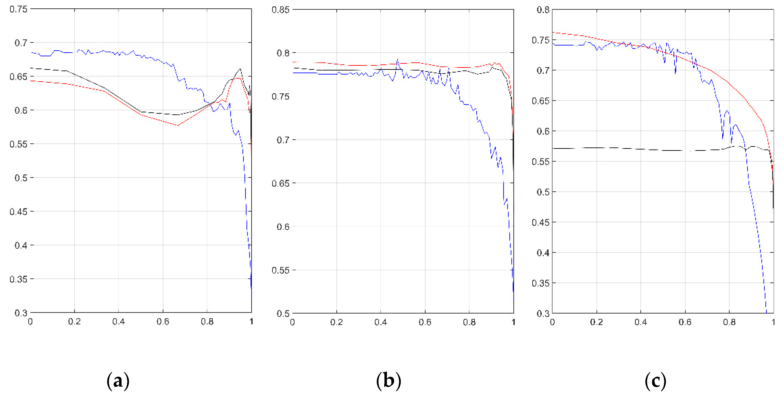
4.3. Feature Selection Experiments with the Information Gain Metric

Our attempts to replicate the feature selection experiments were also fraught with difficulties. Habernal et al. [50] provide very instructive Figures 3–5 and claim that they show the dependence of the macro-F1 measure on feature weight (or score) cut-off value, where the cut-off value ranges from 0 to 1. The interpretation of this setup for the Information Gain metric is that for each cut-off value plotted on the horizontal axis, the graph shows the macro-F1 score obtained by the Maximum Entropy classifier using only the features with at least that level of Information Gain score. Therefore, the higher the cut-off value, the less features remain in the set, and the macro-F1 should gradually decline. This general decreasing trend can sometimes be reversed when there are too many useless features in the set that introduce harmful noise or otherwise confuse the model. In such a case, provided that we first prune the most irrelevant features, we might instead observe an increase in the macro-F1 with the decreasing number of features (i.e., with the increasing cut-off value on the horizontal axis). This is what Habernal et al. [50] hoped for but actually did not observe, because all their graphs exhibit either a stable or monotonously decreasing trend, barring some apparently random fluctuations.
When we tried to replicate these experiments, we were at first puzzled by the fact that our features only got Information Gain scores below 0.06, as can be seen from the scores of the top-20 features shown in Figure 1. Even when we normalized their scores so that they would span the whole interval [0, 1], our graphs still looked very different from those provided in [50]. Eventually, after a lengthy but futile search for possible errors on our side, we hit upon a possible explanation: perhaps there was an error in the figure description and the horizontal axis in fact displayed the proportion of features that were removed from the feature set, starting with those with the smallest Information Gain scores? Indeed, when we thus plotted our results, our graphs did start to resemble those in Habernal et al. [50].
In Figure 1 we plot both their and our replicated results for all the three datasets under this interpretation of the horizontal axis. For the Facebook dataset (left pane) we see that although our replicated results before and after deduplication (shown as red and black lines, respectively) do not quite reach the maximum values reported in [50] (blue line), they do show a clear local maximum at the cut-off level of about 0.95. This means that only 5% of features with the highest Information Gain scores (corresponding to about 3000 features out of the total of 60,050) need to be used for the best macro-F1 results for this dataset.
For movie reviews from csfd.cz (central pane in Figure 2) there is no such obvious local maximum, but from our replicated results it is again evident that there would be little benefit to using more than 10% of the features with the highest Information Gain score (corresponding in this case to about 9000 out of roughly 92,000 features in total). Finally, for the product reviews from Mall.cz (Figure 1c), there was a big difference between our replicated results depending on whether or not the dataset was de-duplicated. Our results for the full dataset with duplicates (red line) mirror quite closely the smoothly descending curve reported in [50] (blue line), and there is no clear cut-off point at which to stop adding or removing features from the feature set in order to reach the best possible macro-F1 score efficiently. In stark contrast to this, the results after deduplication (black line) are dramatically lower due to the removal of massive quantities of duplicates from the dataset. Secondly, although they do not show any obvious local maximum, it is again evident that there would be no benefit in using more than 10% of the features with the highest Information Gain score (corresponding to about 4000 out of roughly 40,000 features in total). Please note that in this last case the deduplication massively reduced the number of features, from about 70,000 for the dataset with duplicates to about 40,000 for the dataset without them. Although duplicates as such do not introduce any new word unigrams or bigrams, they do inflate the frequencies of the existing ones, and thus many more remain in the feature set even after cutting off those that occur less than five times in the corpus (an empirical cut-off level set by Habernal et al. [50] on the basis of other relevant published work).
Because we used different tools, we are not able to explain why Habernal et al. [50] did not observe any local maximum for the Facebook dataset (as they originally expected) and why all their feature selection graphs were so smoothly descending, but at least it shows that they did not deliberately doctor their experimental results to make them conform to their original expectations. It would be very useful if more researchers replicated these feature selection experiments so that some sort of consensus could emerge concerning the optimum number of features to be used for the analysis of these datasets with classical machine learning methods.

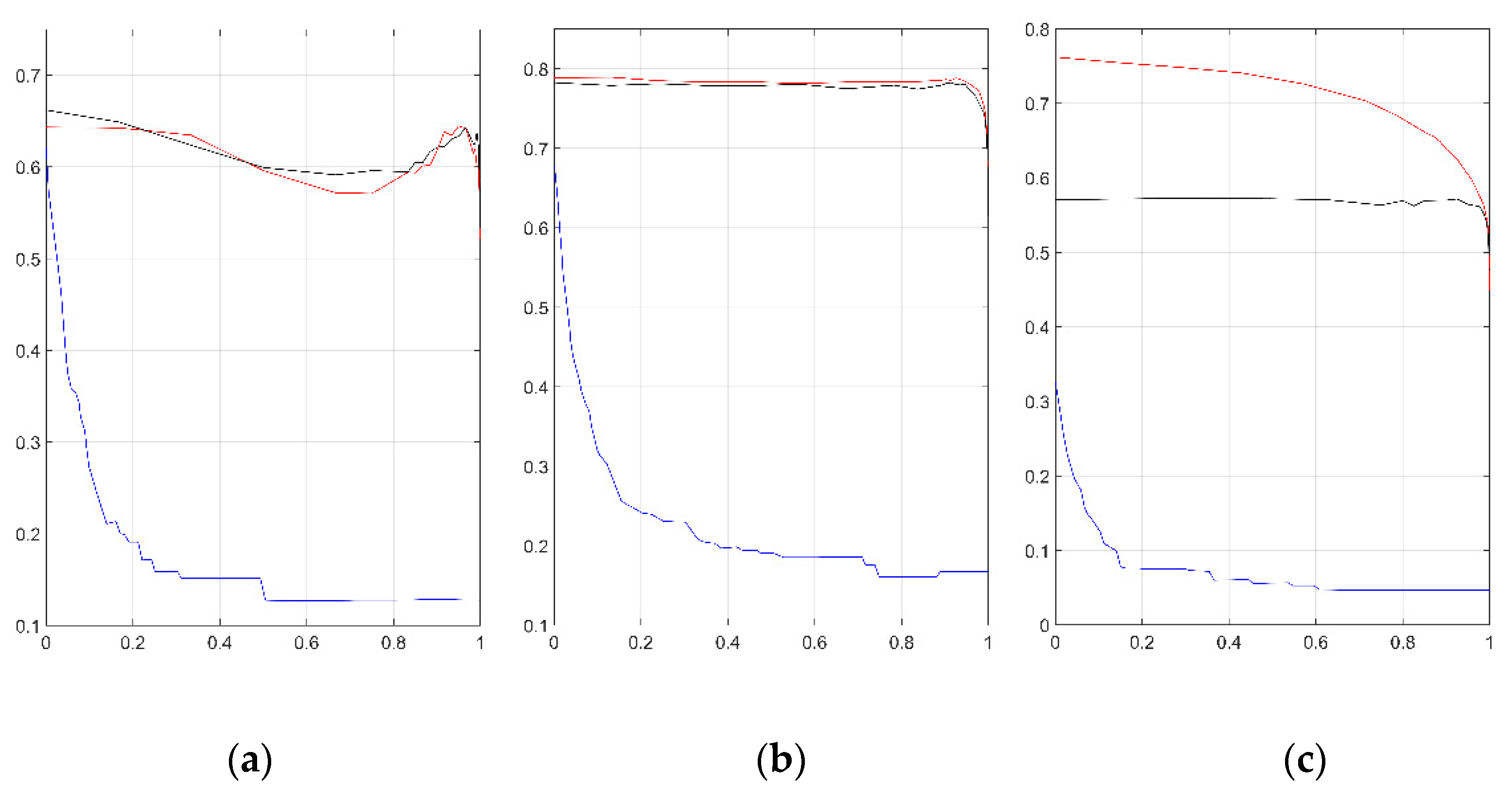
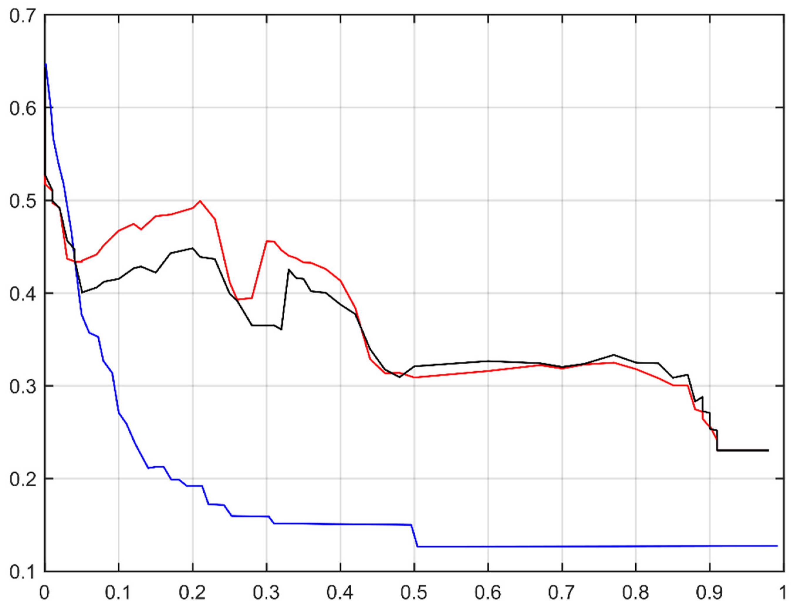
4.4. Feature Selection Experiments with the Chi-Squared Metric

Armed with the knowledge and experience earned in the relatively more straightforward case of the Information Gain, we commenced the investigation of the reported wildly different behavior of the Chi-squared metric. As we suspected all along, the results of our replication experiments in Figure 2 showed that no such “misbehavior” by this metric actually existed; in fact, it behaved nearly the same as the Information Gain.
Our replicated results again show a clear local maximum for the Facebook dataset and uselessness of using more than 10% of the best features in the other two datasets (please note that for product reviews this applies only to the de-duplicated version of the dataset). How then to explain the unexpected and somewhat paradoxical results reported in [50] (reproduced with permission as blue lines in Figure 2)? Again, not having access to their tools and private implementations does not permit us to settle this question with any certainty, but the most likely hypothesis is that there was an implementation error affecting only this metric and probably consisting of erroneously removing the features with the highest Chi-squared scores first (instead of those with the lowest scores).
This might explain why the steepest decline in the macro F1 score was observed right in the beginning near the zero-cut-off value (plotted along the horizontal axis) and, conversely, why there was almost no decline near the maximum cut-off value of 1. In Figure 3, we tried to replicate this suspected human error with both the Chi-squared and the Information Gain metrics and compared our results to those reported for the Chi-squared metric by Habernal et al. [50] in their Figure 5 (chart 5a). Although the match is far from perfect, one could still argue that there seems to be at least a qualitative similarity because all the shown lines decline steeply at first, and then more slowly (albeit in our case with some local maxima, which we conjecture to be caused by mutual correlations between the chunks of added or removed features). In any case, we can now claim with near certainty that the Chi-squared metric is in fact no worse than the others and those who use it can safely continue to do so.

5. Discussion and Methodological Considerations

The preceding sections demonstrate the difficulties we encountered when we tried to use the results reported in Habernal et al. [50] as a baseline for our own research. We at first focused on sentiment classification of Slovak online product reviews into three classes, but irrespective of what we did, our results on Slovak data kept lagging substantially behind that baseline. We eventually managed to resolve this discrepancy by the discovery and removal of large quantities of duplicates from the product review dataset used in [50]. These duplicates accounted for more than 18% of its records, and without deduplication, would seriously distort the performance metric results of any machine learning method. As we report in Section 4.1, after deduplication of “nontrivial” reviews longer than 10 words, the macro-F1 results for this dataset have dropped by more than 19 percentage points. Researchers wishing to use this dataset will, therefore, also have to de-duplicate it before analyzing it. As part of that process, they will have to decide—based on their research goal and wider context—whether the deduplication should be strict (with only one copy of each review permitted in the dataset regardless of its length) or, as we have done in this study, whether they would tolerate the duplicates of shorter reviews as plausibly coming from different customers in response to different products. The good news in this respect was our discovery that the proportion of duplicates in the other two datasets (Facebook and movie reviews) was negligible and so was its effect on their macro-F1 results.
Having thus encountered and resolved the problem with duplicates, we felt motivated to double-check other unexpected results and claims in [50] as well. Two additional noteworthy examples that we identified consisted of the claim that the POS-related features had a highly damaging effect on the macro-F1 score for product reviews (allegedly causing it to drop by more than 19 percentage points), and that the Chi-squared metric was by far the worst and wholly unsuitable for feature selection in sentiment analysis in Czech. In both cases, our replication experiments on the same data (reported in Section 4.2 and Section 4.4) have shown these claims to be wrong: the POS features certainly do not harm sentiment analysis in any way (although they do not seem to help either), and the Chi-squared metric turned out to be as good as the other four metrics, performing in fact on par with the two “winners”, the Information Gain and the Mutual Information.
The main goal behind our replication experiments and error corrections is to make the baseline established by [50] more trustworthy and more widely used. We have noted, for example, that their product review dataset—in stark contrast to the other two—was rarely utilized by other researchers. We suspect that many of them have actually tried to use it, but getting strange results due to its high proportion of duplicates were eventually forced to abandon it. After proper deduplication, this dataset also can become as valuable and widely used as the other two, e.g., to reliably measure the extent of improvement brought about into NLP by the new BERT- and RoBERTa-based neural architectures. We would therefore like to encourage other researchers to also join in these replication efforts in their respective research areas and subareas, just as we have done for sentiment classification of online product reviews into three classes. The resources and baselines provided by Habernal et al. [50] are too valuable to remain underutilized just because some errors may have inadvertently crept into them.
In the remainder of this section we discuss factors affecting the validity and replicability of research results. We start with specific issues encountered in the work of Habernal et al. [50], and then move on to more general aspects including a rather technical but very important case of averaging the F1 measure in cross-validation studies.

5.1. Facilitating Replication of Research Results

With an ever-increasing complexity of problems and tasks tackled by the researchers of Artificial Intelligence it becomes clear that further progress requires global cooperation. Regular replication and validation of experiments by other research teams is an integral part of this effort. To facilitate it as much as possible, researchers need to describe their work in detail and—as far as possible—either use established tools or make their special tools available to others.
In this respect we noted a certain lack of clarity in Habernal et al. [50] concerning some aspects of their tool implementations and modifications, but we warmly appreciate their help, readily extended to us upon request, which enabled us to sufficiently approximate their toolchain for our purposes. Probably the main missing piece of information was the fact that they actually used an SGD (stochastic gradient descent) implementation of the Maximum Entropy algorithm, i.e., the SGD configured with the “log loss” (logistic regression) loss function. Standard implementations of the logistic regression algorithm, which we at first tried, simply took too long to compute for larger numbers of features.
The authors of [50] also did not clearly specify all the hyper-parameters for their algorithms (forcing us to resort to our tool defaults), nor the total numbers of their features. Especially confusing were the missing definitions of their POS-related features where many different combinations and ratios were theoretically possible, but the authors only provided a few illustrative examples rather than a complete list.
Nevertheless, even with some approximation and guesswork on our part, we were able to identify and rectify three major problems present in their work which hindered its more widespread use as a reliable baseline for sentiment analysis in Czech and Slovak:
(a)
Large quantities of duplicates in the product review dataset from Mall.cz that had to be removed prior to analysis;
(b)
Incorrect conclusion that the POS-related features have a detrimental effect on sentiment analysis;
(c)
Incorrect conclusion that the Chi-squared metric is unsuitable for feature selection in sentiment analysis in Czech.
Since we did not replicate the whole extent of their work but focused primarily on the aspects directly relevant to our own research (classification of online product reviews into three classes), it is quite possible that there still remain other, less obvious problems awaiting discovery. We would therefore like to invite other researchers to also partake in these replication efforts, focusing on areas or aspects of direct interest and relevance to their own work.

5.2. On the Comparison of Averaged F1 Scores across Studies

In this section we draw on the work of Forman and Scholz [69] in order to alert researchers to an important problem affecting cross-validation studies using the F1-measure on unbalanced datasets, which is a frequent scenario in NLP and sentiment analysis. Although the F1 measure is “logically” defined as a harmonic mean of precision and recall, it can also be calculated in other ways. In the case of binary classification, which is easiest to explain, it can be alternatively expressed as the function of true positives TP, false positives FP, and false negatives FN, namely F1 = 2.TP/(2.TP + FP + FN). In the context of n-fold cross-validation studies, this translates into three main ways of averaging the F1 scores across folds:
  • The F1 score will be calculated for each fold from the precision and recall for that fold and then averaged;
  • Precision and recall will be calculated for each fold, then averaged, and, finally, the “average” F1 will be calculated as a harmonic mean of the averaged values of precision and recall;
  • True positives TP, false positives FP, and false negatives FN will be calculated for each fold, then averaged, and the “average” F1 will be calculated from their averages through the alternative formula.
Due to nonlinearity inherent in the F1 definition, these three ways of averaging it are not equivalent and can give vastly different results for highly unbalanced datasets. Forman and Scholz [69] provide a very instructive example (in their Table 1 in Section 3.1) with 1504 data rows and 1% (i.e., 15) of positives, to which they apply stratified four-fold cross-validation. Stratification means that each of the four folds will contain three or four examples of the positive class and 372 or 373 examples of the negative class. Assuming a high (but not unrealistic) variation in the model precision (from 24 to 100%) and recall (from 75 to 100%) across individual folds, the authors show that the average F1 can vary from 58 to 73% depending on which of the three ways listed above is used for calculation. It means that, for highly unbalanced datasets, even with the same fold-wise results and ground-truth reality, the estimates of average F1 can differ by more than ten percentage points purely based on how the used tools implement the F1 averaging!
This situation can get even worse when the trained model happens to assign all test set records in some fold to the negative class. This is again rare but not impossible, and it forces the precision (and consequently the F1) for that fold to become undefined. It is important to note here that the third method of averaging the F1 on the basis of the alternative formula with TP, FP and FN is not affected by this problem, because the number of false negatives FN must then be greater than zero—in fact equal to the number of real positives, since they must all have been misclassified as false negatives FN. The denominator (2.TP + FP + FN) in the alternative formula will therefore remain greater than zero, causing the F1 to stay well-defined and equal to zero. In contrast, the first two methods have either to ignore such “failing” folds, or arbitrarily assign to them F1 = 0 and include them in the average F1. In the case of failing folds the number of different ways of calculating the average F1 thus expands to five, depending on how the “failing” folds are handled. Along this line, the authors provide a slightly modified example (in their Table 2) with one failing fold and show that this can lead to an even higher variation in the average F1, in this case from 67 to 91%. Unsurprisingly, ignoring the failing folds turns out to be the worst possible decision, incorrectly inflating the average F1 the most.
Overall, the best method of averaging the F1 across folds—the most robust and least biased even on strongly unbalanced datasets—turns out to be the third one, using the alternative formula. The authors therefore recommend that the developers of machine and deep learning tools start implementing the F1 calculations in this alternative and robust way. Until that happens, however, the researchers and users of their tools face something of a dilemma: the implementation details are often opaque to them, so they are not able to find out how their tool calculates the F1 under cross-validation. They are even less able to say how the F1 was calculated in other published literature against which they may wish to compare themselves. In such situations (which includes our own case), the only practical solution seems to be to try to replicate the published experiments as closely as possible in their own tools and use these replicated results as a baseline against which they will compare their new or improved methods and results. Hopefully this situation will not last long, and new versions of machine and deep learning tools will become more transparent regarding their performance metric calculations for cross-validation studies. (Interested readers can find additional information and guidance on learning from imbalanced datasets in Raeder, Forman and Chawla [74].)

6. Conclusions and Future Work

In this article we replicated several experiments from Habernal et al. [50], which represents the most detailed and comprehensive exploration of supervised machine learning, feature selection, and data pre-processing methods for sentiment analysis of Czech social media undertaken to date. Due to its comprehensiveness, it often serves as a baseline for other sentiment analysis studies not only in Czech, but thanks to their close similarity, also in Slovak. Moreover, Habernal et al. [50] also collected three valuable datasets of opinionated online texts in Czech—Facebook comments, product reviews from Mall.cz, and movie reviews from csfd.cz—and made them freely available to other researchers at http://liks.fav.zcu.cz/sentiment/ (accessed on 17 October 2022). The size of these datasets outstripped earlier such efforts by an order of magnitude, and they have in fact remained a popular and almost unrivalled data resource among researchers to this day. We believe that our replication experiments and the resulting error corrections elaborated in Section 4 will help to make this baseline even more trustworthy and widely used. In order to reap maximum benefit from it, we would recommend the concerned researchers to also heed methodological considerations that we reiterated in Section 5.
Regarding future work, arguably the best possible use of a reliable baseline for sentiment analysis in Czech and Slovak would be to quickly reduce the gap separating these under-resourced languages from the vanguard of sentiment analysis research taking place mostly in English. Since sentiment analysis in its most advanced aspect-based form is, in the words of Bing Liu [7], “a mini-version of the full NLP or a special case of the full NLP … [because] every subproblem of NLP is also a subproblem of sentiment analysis, and vice versa … [including] lexical semantics, coreference resolution, word sense disambiguation, discourse analysis, information extraction, and semantic analysis”, any significant progress in sentiment analysis would naturally translate into a significant progress for NLP in general. Although sentiment analysis is traditionally associated only with specific kinds of data, such as Facebook comments and online product or movie reviews, its potential uses extend far beyond this narrow province. Thus, for example, in one of our national research projects dealing with composable scientific workflows and data processing pipelines (APVV-20-0571 iControl), we contemplate its application to end-user feedback concerning the utility of individual workflow and pipeline elements or modules, to enable artificial intelligence to decide which of several available implementations of a given algorithm to choose for the best results.

Author Contributions

Data curation, J.M.; Formal analysis, P.K., M.K. and L.S.; Methodology, P.K. and M.K.; Project administration, L.H.; Resources, J.M.; Software, J.M. and P.K.; Supervision, L.H.; Validation, P.K., M.K. and L.S.; Writing—original draft, M.K.; Writing—review and editing, J.M., M.K. and P.K. All authors have read and agreed to the published version of the manuscript.

Funding

This work was supported by the Slovak Research and Development Agency under the Contract no. APVV-20-0571 (iControl) and by the projects VEGA Nos. 2/0155/19 and 2/0125/20.

Data Availability Statement

We have used the three datasets made public by Habernal et al. [50] and available at https://liks.fav.zcu.cz/sentiment/ (accessed on 17 October 2022). Prospective users should check for the presence of duplicates before analyzing these datasets.

Acknowledgments

We would like to express our thanks to Habernal et al. [50] for providing the publicly available datasets with opinionated texts in Czech from Facebook, CSFD.cz and Mall.cz, and also for their readiness to answer our questions on the Maximum Entropy implementation, especially for an important piece of information that SGD model was actually used instead of the classical (and slow) Maximum Entropy algorithm. Our work was also supported by the Slovak Research and Development Agency under the Contract no. APVV-20-0571 (iControl) and by the projects VEGA Nos. 2/0155/19 and 2/0125/20.

Conflicts of Interest

The authors declare no conflict of interest.

References

  1. Pang, B.; Lee, L.; Vaithyanathan, S. Thumbs up? Sentiment classification using machine learning techniques. arXiv 2002, arXiv:cs/0205070. [Google Scholar]
  2. Turney, P.D. Thumbs up or thumbs down? Semantic orientation applied to unsupervised classification of reviews. arXiv 2002, arXiv:cs/0212032. [Google Scholar]
  3. Turney, P.D.; Littman, M.L. Measuring praise and criticism: Inference of semantic orientation from association. ACM Trans. Inf. Syst. (Tois) 2003, 21, 315–346. [Google Scholar] [CrossRef] [Green Version]
  4. Dave, K.; Lawrence, S.; Pennock, D.M. Mining the peanut gallery: Opinion extraction and semantic classification of product reviews. In Proceedings of the 12th International Conference on World Wide Web, Budapest, Hungary, 20–24 May 2003; pp. 519–528. [Google Scholar]
  5. Mäntylä, M.V.; Graziotin, D.; Kuutila, M. The evolution of sentiment analysis—A review of research topics, venues, and top cited papers. Comput. Sci. Rev. 2018, 27, 16–32. [Google Scholar] [CrossRef] [Green Version]
  6. Liu, B. Sentiment analysis and opinion mining. Synth. Lect. Hum. Lang. Technol. 2012, 5, 1–167. [Google Scholar]
  7. Liu, B. Sentiment Analysis: Mining Opinions, Sentiments, and Emotions; Cambridge University Press: Cambridge, UK, 2020. [Google Scholar]
  8. Pang, B.; Lee, L. Opinion mining and sentiment analysis. Found. Trends® Inf. Retr. 2008, 2, 1–135. [Google Scholar] [CrossRef] [Green Version]
  9. Tang, H.; Tan, S.; Cheng, X. A survey on sentiment detection of reviews. Expert Syst. Appl. 2009, 36, 10760–10773. [Google Scholar] [CrossRef]
  10. Tsytsarau, M.; Palpanas, T. Survey on mining subjective data on the web. Data Min. Knowl. Discov. 2012, 24, 478–514. [Google Scholar] [CrossRef]
  11. Ekman, P.; Friesen, W.V.; Ellsworth, P. What emotion categories or dimensions can observers judge from facial behavior? In Emotions in the Human Face, 2nd ed.; Ekman, P., Ed.; Cambridge University Press: Cambridge, UK, 1982; pp. 39–55. [Google Scholar]
  12. Fahrni, A.; Klenner, M. Old wine or warm beer: Target-specific sentiment analysis of adjectives. In AISB 2008 Convention Communication, Interaction and Social Intelligence 1–4 April 2008; The Society for the Study of Artificial Intelligence and Simulation of Behaviour: Brighton, UK, 2008. [Google Scholar]
  13. Pang, B.; Lee, L. Seeing stars: Exploiting class relationships for sentiment categorization with respect to rating scales. arXiv 2005, arXiv:cs/0506075. [Google Scholar]
  14. Hazarika, B.; Chen, K.; Razi, M. Are numeric ratings true representations of reviews? A study of inconsistency between reviews and ratings. Int. J. Bus. Inf. Syst. 2021, 38, 85–106. [Google Scholar] [CrossRef]
  15. Batista, H.R.; Junior JC, G.; Miranda, M.D.; Martiniano, A.; Sassi, R.J.; Gaspar, M.A. “If We Only Knew How You Feel”—A Comparative Study of Automated vs. Manual Classification of Opinions of Customers on Digital Media. Soc. Netw. 2018, 8, 74–83. [Google Scholar] [CrossRef] [Green Version]
  16. Stone, P.J.; Dunphy, D.C.; Smith, M.S. The General Inquirer: A Computer Approach to Content Analysis; M.I.T. Press: Cambridge, MA, USA, 1966. [Google Scholar]
  17. Strapparava, C.; Valitutti, A. Wordnet affect: An affective extension of wordnet. Lrec 2004, 4, 40. [Google Scholar]
  18. Esuli, A.; Sebastiani, F. Sentiwordnet: A publicly available lexical resource for opinion mining. In Proceedings of the Fifth International Conference on Language Resources and Evaluation (LREC’06), Genoa, Italy, 22–28 May 2006. [Google Scholar]
  19. Mohammad, S.; Turney, P. Emotions evoked by common words and phrases: Using mechanical turk to create an emotion lexicon. In Proceedings of the NAACL HLT 2010 Workshop on Computational Approaches to Analysis and Generation of Emotion in Text, Los Angeles, CA, USA, 5 June 2010; pp. 26–34. [Google Scholar]
  20. Machova, K.; Marhefka, L. Opinion classification in conversational content using n-grams. In Recent Developments in Computational Collective Intelligence; Springer: Cham, Switzerland, 2014; pp. 177–186. [Google Scholar]
  21. Church, K.; Hanks, P. Word association norms, mutual information, and lexicography. Comput. Linguist. 1990, 16, 22–29. [Google Scholar]
  22. Kim, S.M.; Hovy, E. Determining the sentiment of opinions. In Proceedings of the COLING 2004: Proceedings of the 20th International Conference on Computational Linguistics, Geneva, Switzerland, 23–27 August 2004; pp. 1367–1373. [Google Scholar]
  23. Hu, M.; Liu, B. Mining and summarizing customer reviews. In Proceedings of the Tenth ACM SIGKDD International Conference on Knowledge Discovery and Data Mining, Seattle, WA, USA, 22–25 August 2004; pp. 168–177. [Google Scholar]
  24. Kamps, J.; Marx, M.; Mokken, R.J.; De Rijke, M. Using WordNet to measure semantic orientations of adjectives. Lrec 2004, 4, 1115–1118. [Google Scholar]
  25. Osherenko, A.; André, E. Lexical affect sensing: Are affect dictionaries necessary to analyze affect? In Proceedings of the International Conference on Affective Computing and Intelligent Interaction, Lisbon, Portugal, 12–14 September 2007; Springer: Berlin/Heidelberg, Germany, 2007; pp. 230–241. [Google Scholar]
  26. Machova, K.; Mach, M.; Vasilko, M. Comparison of machine learning and sentiment analysis in detection of suspicious online reviewers on different type of data. Sensors 2021, 22, 155. [Google Scholar] [CrossRef] [PubMed]
  27. Mohamad Sham, N.; Mohamed, A. Climate Change Sentiment Analysis Using Lexicon, Machine Learning and Hybrid Approaches. Sustainability 2022, 14, 4723. [Google Scholar] [CrossRef]
  28. Palomino, M.A.; Aider, F. Evaluating the Effectiveness of Text Pre-Processing in Sentiment Analysis. Appl. Sci. 2022, 12, 8765. [Google Scholar] [CrossRef]
  29. Ruz, G.A.; Henríquez, P.A.; Mascareño, A. Bayesian Constitutionalization: Twitter Sentiment Analysis of the Chilean Constitutional Process through Bayesian Network Classifiers. Mathematics 2022, 10, 166. [Google Scholar] [CrossRef]
  30. Reshi, A.A.; Rustam, F.; Aljedaani, W.; Shafi, S.; Alhossan, A.; Alrabiah, Z.; Ahmad, A.; Alsuwailem, H.; Almangour, T.A.; Alshammari, M.A.; et al. COVID-19 Vaccination-Related Sentiments Analysis: A Case Study Using Worldwide Twitter Dataset. Healthcare 2022, 10, 411. [Google Scholar] [CrossRef]
  31. Tesfagergish, S.G.; Kapočiūtė-Dzikienė, J.; Damaševičius, R. Zero-Shot Emotion Detection for Semi-Supervised Sentiment Analysis Using Sentence Transformers and Ensemble Learning. Appl. Sci. 2022, 12, 8662. [Google Scholar] [CrossRef]
  32. Li, R.; Chen, H.; Feng, F.; Ma, Z.; Wang, X.; Hovy, E. Dual graph convolutional networks for aspect-based sentiment analysis. In Proceedings of the 59th Annual Meeting of the Association for Computational Linguistics and the 11th International Joint Conference on Natural Language Processing, Virtual, 1–6 August 2021; Volume 1, pp. 6319–6329. [Google Scholar]
  33. Tian, Y.; Chen, G.; Song, Y. Enhancing aspect-level sentiment analysis with word dependencies. In Proceedings of the 16th Conference of the European Chapter of the Association for Computational Linguistics: Main Volume, Online, 19–23 April 2021; pp. 3726–3739. [Google Scholar]
  34. Mujahid, M.; Lee, E.; Rustam, F.; Washington, P.B.; Ullah, S.; Reshi, A.A.; Ashraf, I. Sentiment analysis and topic modeling on tweets about online education during COVID-19. Appl. Sci. 2021, 11, 8438. [Google Scholar] [CrossRef]
  35. Moreno, A.; Iglesias, C.A. Understanding Customers’ Transport Services with Topic Clustering and Sentiment Analysis. Appl. Sci. 2021, 11, 10169. [Google Scholar] [CrossRef]
  36. Bacco, L.; Cimino, A.; Dell’Orletta, F.; Merone, M. Explainable sentiment analysis: A hierarchical transformer-based extractive summarization approach. Electronics 2021, 10, 2195. [Google Scholar] [CrossRef]
  37. Lovera, F.A.; Cardinale, Y.C.; Homsi, M.N. Sentiment Analysis in Twitter Based on Knowledge Graph and Deep Learning Classification. Electronics 2021, 10, 2739. [Google Scholar] [CrossRef]
  38. Ligthart, A.; Catal, C.; Tekinerdogan, B. Systematic reviews in sentiment analysis: A tertiary study. Artif. Intell. Rev. 2021, 54, 4997–5053. [Google Scholar] [CrossRef]
  39. Hartmann, J.; Heitmann, M.; Siebert, C.; Schamp, C. More than a feeling: Accuracy and application of sentiment analysis. Int. J. Res. Mark. 2022, in press. [Google Scholar] [CrossRef]
  40. Devlin, J.; Chang, M.W.; Lee, K.; Toutanova, K. Bert: Pre-training of deep bidirectional transformers for language understanding. arXiv 2018, arXiv:1810.04805. [Google Scholar]
  41. Liu, Y.; Ott, M.; Goyal, N.; Du, J.; Joshi, M.; Chen, D.; Levy, O.; Lewis, M.; Zettlemoyer, L.; Stoyanov, V. Roberta: A robustly optimized BERT pretraining approach. arXiv 2019, arXiv:1907.11692. [Google Scholar]
  42. Lehečka, J.; Švec, J.; Ircing, P.; Šmídl, L. Bert-based sentiment analysis using distillation. In Proceedings of the International Conference on Statistical Language and Speech Processing, Cardiff, UK, 14–16 October 2020; Springer: Cham, Switzerland; pp. 58–70. [Google Scholar]
  43. Straka, M.; Náplava, J.; Straková, J.; Samuel, D. RobeCzech: Czech RoBERTa, a monolingual contextualized language representation model. In International Conference on Text, Speech, and Dialogue; Springer: Cham, Switzerland; pp. 197–209.
  44. Sido, J.; Pražák, O.; Přibáň, P.; Pašek, J.; Seják, M.; Konopík, M. Czert--Czech BERT-like Model for Language Representation. arXiv 2021, arXiv:2103.13031. [Google Scholar]
  45. Pikuliak, M.; Grivalský, Š.; Konôpka, M.; Blšták, M.; Tamajka, M.; Bachratý, V.; Šimko, M.; Balážik, P.; Trnka, M.; Uhlárik, F. SlovakBERT: Slovak Masked Language Model. arXiv 2021, arXiv:2109.15254. [Google Scholar]
  46. Hupkes, D.; Veldhoen, S.; Zuidema, W. Visualisation and ‘diagnostic classifiers’ reveal how recurrent and recursive neural networks process hierarchical structure. J. Artif. Intell. Res. 2018, 61, 907–926. [Google Scholar] [CrossRef]
  47. Conneau, A.; Kruszewski, G.; Lample, G.; Barrault, L.; Baroni, M. What you can cram into a single vector: Probing sentence embeddings for linguistic properties. arXiv 2018, arXiv:1805.01070. [Google Scholar]
  48. Hewitt, J.; Manning, C.D. A structural probe for finding syntax in word representations. In Proceedings of the 2019 Conference of the North American Chapter of the Association for Computational Linguistics: Human Language Technologies, Minneapolis, MN, USA, 2–7 June 2019; Volume 1, pp. 4129–4138. [Google Scholar]
  49. Reif, E.; Yuan, A.; Wattenberg, M.; Viegas, F.B.; Coenen, A.; Pearce, A.; Kim, B. Visualizing and measuring the geometry of BERT. Advances in Neural Information Processing Systems 32: Annual Conference on Neural Information Processing Systems 2019, NeurIPS 2019, Vancouver, BC, Canada, 8–14 December 2019. [Google Scholar]
  50. Habernal, I.; Ptáček, T.; Steinberger, J. Supervised sentiment analysis in Czech social media. Inf. Process. Manag. 2014, 50, 693–707. [Google Scholar] [CrossRef]
  51. Veselovská, K. Sentiment Analysis in Czech; Ústav Formální a Aplikované Lingvistiky, ÚFAL MFF UK: Praha, Czech Republic, 2017. [Google Scholar]
  52. Klimešová, P. Sentiment Analysis with Linguistic Knowledge. Bachelor’s Thesis, Faculty of Informatics, Masaryk University, Brno, Czech Republic, 2022. Available online: https://is.muni.cz/th/n0lnb/Sentiment_Analysis_cz.pdf (accessed on 17 October 2022).
  53. Smrž, P. Using WordNet for opinion mining. In Proceedings of the Third International WordNet Conference, Seogwipo, Korea, 22–26 January 2006; pp. 333–335. [Google Scholar]
  54. Smrž, P. Automatic acquisition of semantics-extraction patterns. In Proceedings of the Fifth International Conference on Language Resources and Evaluation (LREC’06), Genoa, Italy, 22–28 May 2006. [Google Scholar]
  55. Žižka, J.; Dařena, F. Automatic sentiment analysis using the textual pattern content similarity in natural language. In Proceedings of the International Conference on Text, Speech and Dialogue, Brno, Czech Republic, 6–10 September 2010; Springer: Berlin/Heidelberg, Germany; pp. 224–231. [Google Scholar]
  56. Veselovská, K.; Hajic, J.; Sindlerová, J. Creating annotated resources for polarity classification in Czech. In Proceedings of the 11th Conference on Natural Language Processing (KONVENS), Vienna, Austria, 19–21 September 2012; pp. 296–304. [Google Scholar]
  57. Červenec, R. Rozpoznávání emocí v česky psaných textech. Ph.D. Thesis, Fakulta Elektrotechniky a Komunikačních Technologií, Vysoké Učení Technické v Brně, Brno, Czech Republic, 2011. [Google Scholar]
  58. Habernal, I.; Ptáček, T.; Steinberger, J. Sentiment analysis in Czech social media using supervised machine learning. In Proceedings of the 4th Workshop on Computational Approaches to Subjectivity, Sentiment and Social Media Analysis, Atlanta, Georgia, 14 June 2013; pp. 65–74. [Google Scholar]
  59. Habernal, I.; Brychcín, T. Semantic spaces for sentiment analysis. In Proceedings of the International Conference on Text, Speech and Dialogue, Pilsen, Czech Republic, 1–5 September 2013; Springer: Berlin/Heidelberg, Germany; pp. 484–491. [Google Scholar]
  60. Brychcín, T.; Habernal, I. Unsupervised improving of sentiment analysis using global target context. In Proceedings of the International Conference Recent Advances in Natural Language Processing RANLP, Online, 1–3 September 2013; pp. 122–128. [Google Scholar]
  61. Kincl, T.; Novák, M.; Přibil, J.; Štrach, P. Language-independent sentiment analysis with surrounding context extension. In Proceedings of the International Conference on Social Computing and Social Media, Los Angeles, CA, USA, 2–7 August 2015; Springer: Cham, Switzerland, 2015; pp. 158–168. [Google Scholar]
  62. Lenc, L.; Hercig, T. Neural Networks for Sentiment Analysis in Czech. In Proceedings of the ITAT, Tatranské Matliare, Slovakia, 15–19 September 2016; pp. 48–55. [Google Scholar]
  63. Hercig, T.; Krejzl, P.; Hourová, B.; Steinberger, J.; Lenc, L. Detecting Stance in Czech News Commentaries. In Proceedings of the ITAT, Martinské Hole, Slovakia, 22–26 September 2017; pp. 176–180. [Google Scholar]
  64. Libovický, J.; Rosa, R.; Helcl, J.; Popel, M. Solving Three Czech NLP Tasks with End-to-end Neural Models. In Proceedings of the ITAT, Plejsy, Slovakia, 21–25 September 2018; pp. 138–143. [Google Scholar]
  65. Cano, E.; Bojar, O. Sentiment analysis of Czech texts: An algorithmic survey. arXiv 2019, arXiv:1901.02780. [Google Scholar]
  66. Krchnavy, R.; Simko, M. Sentiment analysis of social network posts in Slovak language. In Proceedings of the 2017 12th International Workshop on Semantic and Social Media Adaptation and Personalization (SMAP), Bratislava, Slovakia, 9–10 July 2017; IEEE: Piscataway, NJ, USA, 2017; pp. 20–25. [Google Scholar]
  67. Pecar, S.; Simko, M.; Bielikova, M. Sentiment analysis of customer reviews: Impact of text pre-processing. In Proceedings of the 2018 World Symposium on Digital Intelligence for Systems and Machines (DISA), Košice, Slovakia, 23–25 August 2018; IEEE: Piscataway, NJ, USA, 2018; pp. 251–256. [Google Scholar]
  68. Pecar, S.; Šimko, M.; Bielikova, M. Improving sentiment classification in Slovak language. In Proceedings of the 7th Workshop on Balto-Slavic Natural Language Processing, Florence, Italy, 2 August 2019; pp. 114–119. [Google Scholar]
  69. Forman, G.; Scholz, M. Apples-to-apples in cross-validation studies: Pitfalls in classifier performance measurement. ACM Sigkdd Explor. Newsl. 2010, 12, 49–57. [Google Scholar] [CrossRef]
  70. Korenek, P.; Šimko, M. Sentiment analysis on microblog utilizing appraisal theory. World Wide Web 2014, 17, 847–867. [Google Scholar] [CrossRef]
  71. Risch, J.; Krestel, R. Delete or not delete? Semi-automatic comment moderation for the newsroom. In Proceedings of the First Workshop on Trolling, Aggression and Cyberbullying (TRAC-2018), Santa Fe, NM, USA, 25 August 2018; pp. 166–176. [Google Scholar]
  72. Balogh, Š.; Mojžiš, J.; Krammer, P. Evaluation of System Features Used for Malware Detection. In Proceedings of the Future Technologies Conference, Vancouver, BC, Canada, 28–29 November 2021; Springer: Cham, Switzerland; pp. 46–59. [Google Scholar]
  73. Sabo, R.; Krammer, P.; Mojžiš, J.; Kvassay, M. Identification of Spontaneous Spoken Texts in Slovak. Jazykoved. Cas. 2019, 70, 481–490. [Google Scholar] [CrossRef]
  74. Raeder, T.; Forman, G.; Chawla, N.V. Learning from imbalanced data: Evaluation matters. In Data Mining: Foundations and Intelligent Paradigms; Springer: Berlin/Heidelberg, Germany, 2012; pp. 315–331. [Google Scholar]
Figure 1. Feature selection experiments with the Maximum Entropy classifier and the Information Gain metric for (a) the Facebook dataset, (b) Movie reviews from CSFD.cz, and (c) Product reviews from Mall.cz. Blue lines in all the charts correspond to the macro-F1 results reported by Habernal et al. [50] and are reproduced here with permission from their Figures 5b, 4b, and 3b, respectively. Red lines correspond to our replication of their experiments on the datasets with duplicates, black lines to our experiments on the de-duplicated versions of the datasets. Horizontal axis is interpreted as showing the proportion of features with the lowest Information Gain scores that were removed from the feature set before measuring the macro-F1.
Futureinternet 14 00300 g001
Figure 2. Feature selection experiments with the Maximum Entropy classifier and the Chi-Squared metric for (a) the Facebook dataset, (b) Movie reviews from csfd.cz, and (c) Product reviews from Mall.cz. Blue lines in all the charts correspond to the macro-F1 results reported by Habernal et al. [50] and are reproduced here with permission from their Figures 5b, 4b, and 3b, respectively. Red lines correspond to our replication of their experiments on the datasets with duplicates, black lines to our experiments on the de-duplicated versions of the datasets. Horizontal axis is interpreted as showing the proportion of features with the lowest Chi-Squared scores that were removed from the feature set before measuring the macro-F1.
Futureinternet 14 00300 g002
Figure 3. Results of our deliberately “inverted” feature selection experiments with the Maximum Entropy classifier, and both the Chi-Squared (red line) and the Information Gain metric (black line) for the full Facebook dataset with duplicates. In these experiments, we first removed the features with the highest scores. The blue line corresponds to the results of standard (not inverted) feature selection experiments with the Chi-squared metric reported by Habernal et al. [50]; it is reproduced here, with permission, from their Figure 5a. In all the cases, the horizontal axis is to be interpreted as showing the proportion of features removed from the feature set before measuring the macro-F1.
Futureinternet 14 00300 g003
Table 1. Illustrative examples from the three datasets provided by Habernal et al. [50]. Approximate English translations shown here are not part of the datasets.
ClassTextApproximate English Translation (Not Part of the Dataset)
Facebook dataset
Negativeani náhodou...not even by chance…
Negativety šaty kdo jim navrhnul byl asi vožralejThe designer of their clothes must have been drunk
PositiveMám ji je skvělá!I have it it’s great!
Positivemoje nejoblíbenější!!!my favourite!!!
Neutralnajde se nějaký sponzor?any sponsors around here?
Neutralto mam doma:-D asi to začnu používat když to stojí tolik:-DI have that at home:-D I guess I will start using it since it costs so much:-D
Movie reviews from csfd.cz
Negativetak toto se opravdu nepovedloso this really did not work out well
NegativeMoc, ale moc špatný...Really, but really bad…
PositiveJednoduše geniální.Simply genius.
PositiveFilm mého dětství. Super.The film of my childhood. Super.
Neutral...a půl hvězdičky Vašíkovi Neckářovi...... and a half-star to Vašík Neckář...
NeutralFilm o ničem... s dobrými herci, ale o ničem.!Film about nothing… with good actors, but about nothing.!
Product reviews from Mall.cz
Negativevadí mi, že intenzata vůně brzy vyprchá.it bothers me that the intensity of the fragrance evaporates soon.
NegativeČekala jsem od tohoto výrobku více.I expected more from this product.
Positivesplnilo očekávání, výborný na cestyfulfilled expectations, excellent for travel
PositiveSkvělý pomocník při údržbě pračky.Excellent helper for washing machine maintenance.
NeutralJe hlučnější, ale pro domásí použití dostačuje.It is a bit noisy but will do for home use.
NeutralCelkem spokojenost, i když stabilita není zas až tak úžasná.Overall satisfaction, although its stability is not overwhelming…
Table 2. Data pre-processing techniques, feature types and feature selection methods evaluated in Habernal et al. (2014).
Data Pre-Processing TechniquesFeature TypesFeature Selection Methods
TokenizingWord unigramsChi-Squared
POS TaggingWord bigramsInformation Gain
Named Entity FilteringCharacter n-gramsMutual Information
StemmingPOS-related featuresOdds Ratio
LemmatizationEmoticonsRelevancy Score
Stop-word RemovalDelta TFIDF variants (only as an alternative to word unigrams in binary classification)
Lowercasing
Phonetic transcription
Table 7. Top-20 Features with the highest Information Gain scores for the Facebook and the Mall.cz datasets (with duplicates).
Facebook with DuplicatesMall.cz with Duplicates
IG ScoreFeature NameIG ScoreFeature Name
5.31542105 × 10⁻²pos_VN_cnt2.29515576 × 10−2jinak_27
5.31542105 × 10⁻²pos_VN_rel1.39020370 × 10−2pos_Z_cnt
4.82305556 × 10⁻²pos_A_rel1.38809112 × 10−2spokojen_1
3.00267410 × 10⁻²pos_P_cnt1.27684311 × 10−2bohužel_129
2.93030264 × 10⁻²krás_171.21083059 × 10−2troch_39
2.79489530 × 10⁻²pos_J_rel1.17427526 × 10−2že_5
2.79405964 × 10⁻²pos_V_cnt1.06867967 × 10−2pos_VN_rel
2.79336596 × 10⁻²pos_J_cnt1.06843420 × 10−2pos_VN_cnt
2.74006129 × 10⁻²pos_N_cnt1.01632063 × 10−2doporučuj_3
2.31843806 × 10⁻²pos_R_cnt9.90660242 × 10³pos_N_cnt
2.31843806 × 10⁻²pos_R_rel9.88890573 × 10³špatn_148
2.04175911 × 10⁻²nejlepší_289.70657370 × 10³pos_J_cnt
1.81899721 × 10⁻²pos_P_rel9.70657370 × 10³pos_J_rel
1.73519507 × 10⁻²pos_A_cnt9.15182532 × 10³pos_V_cnt
1.62609275 × 10⁻²pos_VD_div8.62281841 × 10³pos_R_rel
1.61785256 × 10⁻²pos_D_cnt8.61252827 × 10³pos_R_cnt
1.56507796 × 10⁻²dobr+den_286757.84887959 × 10³dobr_4
1.54041112 × 10⁻²pos_T_cnt7.75472028 × 10³pos_D_cnt
1.54041112 × 10⁻²pos_T_rel7.35274446 × 10³mohl_65
1.49780643 × 10⁻²super_326.94441155 × 10³pos_T_cnt
Publisher’s Note: MDPI stays neutral with regard to jurisdictional claims in published maps and institutional affiliations.

