
Quantum Clones inside Black Holes


Institute for Theoretical Physics, Utrecht University, Princetonplein 5, 3584 CC Utrecht, The Netherlands
Universe 2022, 8(10), 537; https://doi.org/10.3390/universe8100537
Submission received: 5 September 2022
/
Revised: 13 October 2022
/
Accepted: 13 October 2022
/
Published: 18 October 2022
(This article belongs to the Section Foundations of Quantum Mechanics and Quantum Gravity)
Abstract
A systematic procedure is proposed for better understanding the evolution laws of black holes in terms of pure quantum states. We start with the two opposed regions I and in the Penrose diagram, and study the evolution of matter in these regions, using the algebra derived earlier from the Shapiro effect in quantum particles. Since this spacetime has two distinct asymptotic regions, one must assume that there is a mechanism that reduces the number of states. In earlier work we proposed that region describes the angular antipodes of region I, the ‘antipodal identification’, but this eventually leads to contradictions. Our much simpler proposal is now that all states defined in region are exact quantum clones of those in region I. This indicates more precisely how to restore unitarity by making all quantum states observable, and in addition suggests that generalisations towards other black hole structures will be possible. An apparent complication is that the wave function must evolve with a purely antisymmetric, imaginary-valued Hamiltonian, but this complication can be well-understood in a realistic interpretation of quantum mechanics.
1. Introduction
It has been proposed earlier by this author [1,2] to regard the Penrose diagram for the eternal, time independent black hole as a single pure quantum state, on which one then projects the physical excitations using creation and annihilation operators, so as to obtain the complete spectrum of all pure black hole states that are physically close to the time independent one. These operators, however, do not commute with the observables describing the original collapse of the black hole, let alone its final evaporation, and this is why the effects of collapse and evaporation should not be added to describe the metric for the background of the quantum effects. We usually proceed by removing collapse and evaporation, which restricts us to using the metric of an eternal black hole. Section 2 and Section 3 describe the basic features needed, such as the Kruskal–Szekeres coordinates. Section 4 and Section 5 recapitulate earlier work on the Shapiro effect and its consequences, and on the algebra that ensues if we apply spherical wave expansions for in- and out going matter.
These findings continue not to be universally accepted or appreciated, but they are crucial for understanding this paper. At some point it seems as if we are not counting right. In this paper, we make another attempt to be more precise. The main idea of this paper is treated in Section 6. How our treatment leads to a unitary description of the black hole evolution laws is recapitulated in Section 7. Some of the problems still left wide open are mentioned in Section 8, and we phrase our conclusions in Section 9.
2. The Pure, Time Independent State
Consider the metric of a static black hole; We take it to be considerably larger and heavier than the Planck length and mass:
For simplicity this will be the Schwarzschild solution, but generalisation towards the Reissner–Nordstrom or Kerr–Newman solutions will be straightforward. As is well-known, this solution does not show a black hole surrounded by a vacuum, but it is accompanied by a quantum stream of Hawking particles forming a heat bath for the black hole. The Hawking particles are dominated by a tenuous cloud of particles with masses and energies far below the Planck value, so that, for the outside world, their direct effects on the total metric are negligible, though they will be important when considered over long stretches of time.
In many cases, considering long enough stretches of time, this state is not completely time-independent. If the Hawking particles are only represented by the ones escaping from the hole, the black hole mass decreases. A completely static black hole arises only if the heat bath is carefully tuned to reach perfect time independence. Using standard methods from quantum mechanics, this can be regarded as a time independent superposition of three streams of (free) particles: a beam of out going particles (out-particles), a beam of in going particles (in-particles), and surrounding particles with angular momentum too high to pass through the angular momentum potential barrier (exterior-particles).
An observer close to the intersection point of the future event horizon and the past event horizon, defines the local energy and momentum density in terms of locally flat coordinates. (S)he then experiences a local vacuum there, which is a unique vacuum state, so that, from her point of view, we are dealing with a single pure state. We now borrow this language to say that, also for the outside observers, this may be regarded as a single pure state. We claim that any observer will not be able to distinguish a thermal state from a pure state in thermal equilibrium (a micro-canonical ensemble), so here comes our first postulate:
The state where the local observer sees a local minimum of the energy density, i.e., a local vacuum state, will here be referred to as the Unruh vacuum state [3]; it may be regarded as a pure state. The excited states that we shall use, will in general be time dependent, small deviations from the Unruh state.
3. The Kruskal–Szekeres Coordinates
Now, we consider the analytic continuation of the Schwarzschild metric. Since the local observer sees no particles at all, Einstein’s equations will require that continuation be carried out by assuming strict absence of matter near the black hole. In particular, local observers will see no matter crossing future and past horizons. If angular momentum and electric charge are assumed to be negligible, only the Schwarzschild metric and its analytic extensions will apply, and therefore it is this spacetime that is the only appropriate one for describing the stationary black hole in an Unruh heat bath. We have:
The ideal continued metric is the Kruskal [4]–Szekeres [5] metric. Replacing by , with
one derives that the metric is
This metric is singularity free at the origin, which is at .
Now, a natural procedure is to start from here to define time dependent quantum states, by applying field operators, chosen to be functions of and the angles . Then, however, one obtains too many states, while quantum information appears to be transported across the horizons. Spacetime described by the coordinates features two asymptotic domains rather than one, simply because every point with is associated with one point with and and one point where both x and y are negative.
Our proposal in Refs. [1,2] was to impose a constraint on the physical states: All particle states in the domain are to be identified with the particles on by associating them to the other’s antipodes: .
In this paper, we report about our further attempts to implement this idea in practical calculations. We found ourselves forced to withdraw the latter additional condition; the antipodal states do not match correctly to the parent states, due to the need to impose invariance. A more technical argument for rejecting the antipodal mapping is presented in Appendix A. No antipodal mapping is to be included in the definition of the physical states.
There happens to be a much more natural way to limit the physical states: Only those local operators that are invariant under the exchange , are admitted to define new physical states. We return to this later (Section 6).
The danger of omitting the antipodal mapping is that this removes the protection of our logic against cusp singularities at the origin. We shall have to carefully register what happens there.
To focus into the region , we go to a coordinate frame that describes spacetime there. Write
In these coordinates, we have
4. The Shapiro Effect
Of all forces in nature that could explain how black holes process information going in, into information going out again, the Shapiro effect is the most dramatic one. The Shapiro effect is the phenomenon that a radio signal grazing past the Sun is being slowed down by the Sun’s gravitational field. It is a basic property of the Schwarzschild metric outside the Sun. Any fast moving elementary particle also carries a gravitational field that exerts a Shapiro effect on other particles in its neighbourhood. The effect is computed by subjecting the Schwarzschild metric of a particle at rest, to a strong Lorentz boost. Even if the rest mass of the original particles was negligible (as we shall usually assume), its boosted momentum can easily reach values such that in-particles cause a shift in the positions of the out-particles.
First consider a small, locally flat region of spacetime. In that case, one finds that, whenever an in-particle meets an out-particle on its way, the out-particle undergoes a shift. If the in-particle has momentum in the inwards direction, parallel to the coordinate , then the out particle is dragged along in the direction by an amount , calculated to be:
where is the scattering parameter (the transverse separation of the two particles).
Equation (7) was first derived in flat spacetime [6,7], but it is easy to generalise it to the spacetime (5) very close to a black hole horizon [8]. In that case, we replace the transverse coordinates by the angles . Furthermore, since the displacement is a linear function of the sources, we can arrange all contributions from all in going particles as a convolution:
where is a function of the angular separation between the points and , which indicate where the out- and in-particles both puncture through the horizon. The function f obeys the angular Laplace equation,
Thus, if represents the momentum of an in-particle added to the system, at angular position , then Equation (8) tells us that, all out-particles at position are shifted by an amount . Our next step is to replace this by the following statement: if all in going matter is represented by a function , where i counts the in-particles, then all out-matter is described by the position function , obeying
This relation tells us how out-particles are arranged by the in-particles. With Equation (9), we have
It should be understood that the in-particles are defined by their momenta as they cross the future event horizon.
A very important point is that we omitted the in front of . This is because the (light cone) momentum increases proportionally to , where is the (negative) time coordinate for the outside observer, normalised as in Equation (5). Similarly, out-particles have momenta , decreasing as .
Therefore, it is the relative displacements that are more important than absolute positions, allowing us to redefine the location of the origin of space.
The light-cone positions and of the in- and the out-particles scale with time, , exactly as and do.
5. Spherical Harmonics
It is now instrumental to apply the spherical wave expansion:
where , with , are the usual spherical harmonic functions obeying With these, we find that Equation (11) turns into
where the subscripts in, out, remind the reader that refers to out-particles and refers to in-particles. u are positions, p are momenta.
To date, everything was classical. Now comes quantum mechanics. For the particles, quantum mechanics implies that
and consequently,
note that and have been defined as follows:
so that Equations (15) follow from (14). Defining Equation (13) implies
and furthermore, also the variables
obey while their dependence is generated by the Hamiltonian
which is that of a repulsive harmonic oscillator, as was noted by Betzios, Gaddam and Papadoulaki [9].
6. Clones
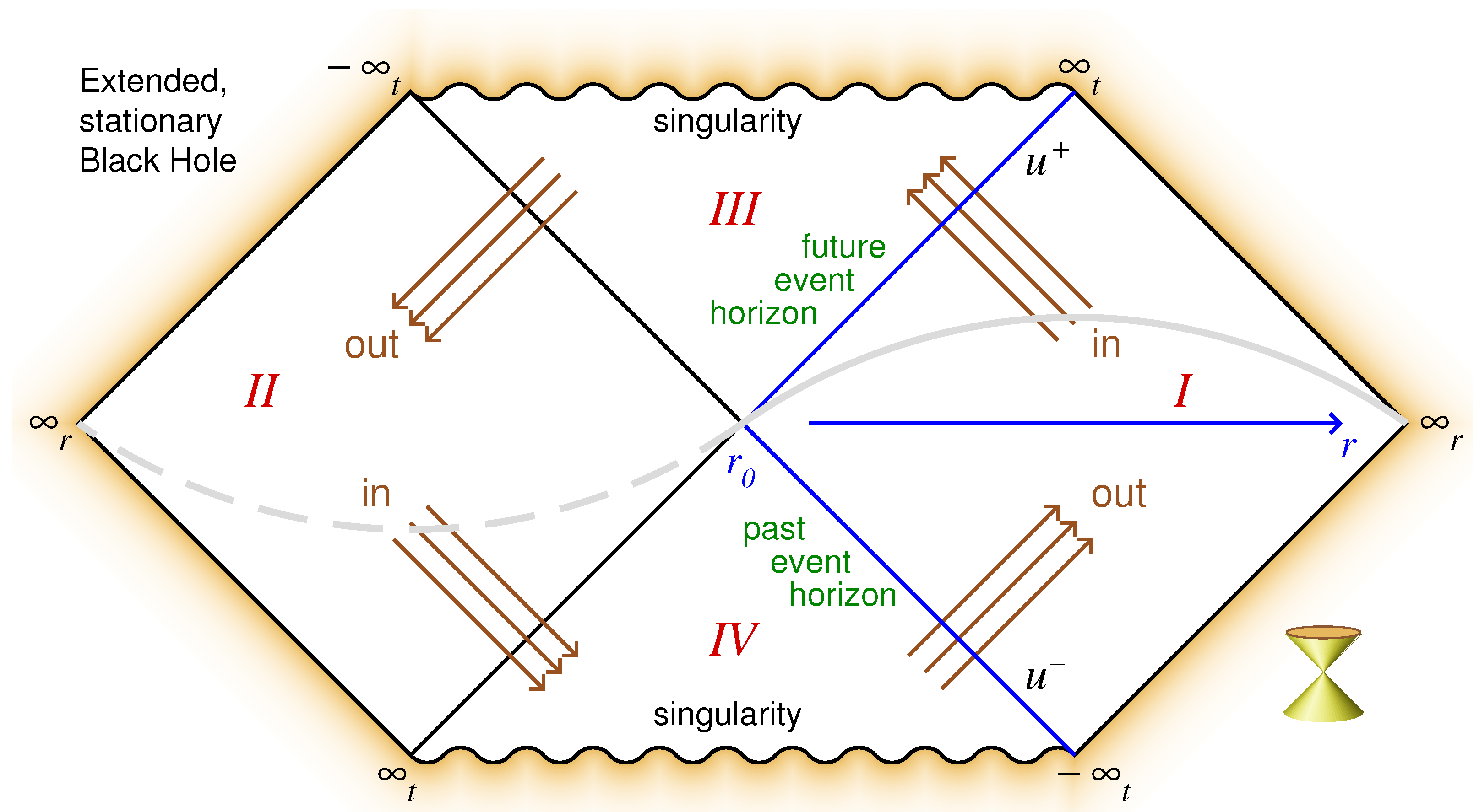
We see that the in-particles punch through the future event horizon either at positive (region I) or at negative (region ), see Figure 1. This figure is a Penrose diagram, obtained by squeezing the coordinates to fit in finite segments, in order to render the entire surrounding universe. The coordinates both span the entire line .
Equations (14)–(17) imply that, at every value for , the wave function for the in-particles, is Fourier transformed to give for the out-particles. Such a Fourier transform is unitary, so this should yield a perfectly unitary relation between the in- and the out-particles.
However, the particles that escape to region are not visible for the observers in region I. This seems to violate unitarity after all. In previous presentations we had assumed that the situation was cured by proposing the particles in region to be nothing but the antipodes of particles in region I. The picture seemed to work very well. For instance, the only spots in the Penrose diagram where particles approach their antipodes closely, are the singularities in regions and , which are outside the domains of physical interest and therefore totally harmless.
Yet, we have to withdraw this proposal, mainly for the following reason: written in the Schwarzschild coordinates , the antipodal mapping used is:
which includes a parity reversal P, possibly with a particle-antiparticle conjugation, C, but no time reversal, T. If, alternatively, we write the transformation in the Kruskal–Szekeres coordinates , the transformation is
In this notation, we have time reversal T without parity change P.
Both pictures do not follow a transformation, the only non-trivial reflection operator for which the Standard Model interactions are completely invariant. This would imply that the two regions I and do not quite evolve the same way, which would be difficult to defend if the entire Penrose diagram would be assumed to describe just different parts of one and the same spacetime. See also our other objection to the antipodal identification, Appendix A.
Rejecting the antipodal mapping brings back to us the danger of a cusp singularity. This we shall deal with in a different way, see Section 7.
One could suppose that, in the Penrose diagram, simply nothing but a pristine vacuum enters region from region at time . In our philosophy, this cannot be right, since region describes the same geometry as region I. It cannot be in a vacuum at all. We should use all particles that cross the future event horizon, and Fourier transform them to become the out going particles. We want the states in region to be exactly the ones needed to make the evolution time reversal symmetric and unitary.
Now let us assume that the particles in region are exact quantum clones of the particles in region I, without the antipodal interchange. At first sight, this seemed to be wrong (which was why it took us so long to get the correct picture!), but let us check.
Quantum clones are defined to be states with exactly the same wave function as some other states. In ordinary circumstances this can practically never arise naturally, but black holes are not natural in this respect. The assumption is now that, all particles in region , are described by the same wave functions as the particles in region I:
The need for complex conjugation here is not obvious, and it was omitted in the earlier versions of this paper. However, let us temporarily accept Equation (20), since invariance does require complex conjugation in this equation. This is because the time evolution in the time variable , defined by Equations (3) and (5) in regions I and , goes in opposite directions (see the Cauchy surface, grey curve, in Figure 1).
The asterisk in Equation (20) will not be without consequences however, because the Fourier transformation relating to does not preserve this constraint. What is going on?
Let , with and real (particles moving with the speed of light through the future event horizon, have wave functions not depending on ). According to Equation (20), is even and is odd in . Then the Fourier transform defined by
This is a real function but it is not even in p, which would be dictated by Equation (20) if would be real.
Therefore, we demand our wave functions to be even in both and and to be real. The first condition would be the statement that the wave function for negative should be a quantum clone of the function for positive . The second condition is less familiar. Can we impose wave functions to be real? What would their Schrödinger equation look like?
From a fundamental point of view, demanding a wave function to be real is easy: just ensure that the Hamiltonian is imaginary, and hence antisymmetric. In fact, we can repair complex wave functions rather easily: complex wave functions are pairs of real wave functions. Real wave functions that occur in pairs actually describe a system with an auxiliary binary variable. The binary variable that we usually have helps us define energy eigen states. In quantum gravity we may still have a conventional Schrödinger equation, but the energy eigen states all come in pairs of positive and negative energy. This seems to be a healthy starting point for more advanced quantum theories. We leave this aspect for future investigations. Right now we can make one interesting remark. The fact that we have no complex wave functions may entail that we have no conserved global charges in our theory. This was to be expected in a theory of black holes.1
7. Unitary Evolution
Now we are in a position to formulate the complete evolution law for a Schwarzschild black hole:
- (1)
- Start with the Schwarzschild metric, Equation (2).
- (2)
- Write the wave functions of the in-particles in terms of the coordinates . These wave functions must be real-valued.
- (3)
- Only the part where is physical. Now define the part for as being the quantum clone of the wave for positive
- (4)
- Find the wave function as the Fourier transform of over the entire stretch of values. Since , this Fourier transform obeys the same constraints as .
- (5)
- As the Hamiltonian must be imaginary and antisymmetric, the wave function in the entire region is a quantum clone of that in region I.
- (6)
- Return to the Schwarzschild coordinates.
This last step is very important. Our wave function is defined in such a way that replacing by yields the same function . Therefore, is also well-defined on the original Schwarzschild coordinates .
Furthermore, now we can return to the cusp singularity. Is there a cusp singularity at the origin? The answer is no. In terms of the Kruskal–Szekeres coordinates our equations are totally regular as there is no singularity of the metric. Unitarity holds, so the wave functions are always normalisable. There may be soft singularities as in other solutions of the wave equations, but these are totally acceptable from physical point of view.
How do we understand unitarity? What happens if the entire system is postulated to obey the algebra of Section 4, if we solve the equations in terms of the spherical harmonics of Section 5?
We now describe the main result of this paper: we can write the evolution equations exclusively in terms of the data in region I only. The calculation does employ the Fourier transformation, but in this formalism it fully respects unitarity. The wave function of particles entering at positive values of while , generates wave functions through Equations (17) and (21), which now take the form
This is entirely unitary. Black hole information is preserved.
To understand how this works in detail, consider the separate evolution equations at given . Since the algebraic equations for different commute, we just need to look at one generic value of (this is no longer the case at very high values of ℓ, where the expansion should be terminated; thus we keep only those ℓ values whose contributions commute).
At these values of ℓ, the operators and act as one-particle position and momentum operators.2 The clone condition means that the wave function for the in-particle needs to be defined only for the values , after which we define the wave function to obey:
This is a subspace of all wave functions that may be considered, but the constraints are necessary for self consistence.
We can now ask how this sub space evolves, when applying the algebra of Section 4. As stated, the Fourier transform is not unitary on half spaces, but let us check this anyway!
The prototypes of the wave functions for the in-particles obeying Equation (23) describe a particle at :
(to be normalised later). Note that may be positive or negative, but a is restricted to be positive.
The out-particle will be the Fourier transform of this. We have
This is again3 an even function of ! Therefore both in space and in space, we can omit the negative halves. The mapping on the half spaces one onto the other is unitary. We have, normalising things correctly on the half-spaces ,
where, again, the subscripts ‘in’ and ‘out’ are merely to remind the reader that the latter inproduct connects the out-states to the in-states. The reader is invited to check that Equations (27) and (28) are mutually compatible in the half-spaces .
Conclusion: by limiting ourselves to the half-spaces , we get a completely unitary transition between the in-particles and the out-particles. This way of seeing how this can happen, by postulating cloning, is new.
In stead of the even functions, we can also choose to use only odd functions. In that case:
One can fix the signs here to be positive, without losing generality, since all values have to be multiplied.
The attentive reader might now ask: wait, if the metric using and as its coordinates, is assumed to carry exactly the cloned quantum states of the coordinates, should we not simply continue by putting the quantum states directly onto the original Schwarzschild coordinates ? Why open up to the Kruskal–Szekeres coordinates at all?
That would be a very good question. We now believe however that there are two issues when studying black holes: (1), the quantum states—to which the question applies, and (2), the evolution law, for which we need the Shapiro delay, and the algebra that follows from it. So the answer to the question is: first open up the metric (i.e., go to the Kruskal–Szekeres coordinates) to display the evolution laws and their algebra as sharply as possible, then close it (i.e., go back to the Schwarzschild coordinates), to establish the boundary conditions. At the boundary, we may assume all quantum states to be in their cloned form, and, as we established in this section, they will stay cloned forever. Knowing this, we can continue using the Schwarzschild coordinates.
The rules for using quantum mechanics, in terms of the states in region only, are unchanged.
8. Miscellaneous Open Problems
8.1. Towards the Black Hole Equations
The problem that we wished to solve is how to derive equations that fully determine the pure quantum states for the out-going particles if we know how the Standard Model (SM) projected the in-particles along the future event horizon. The SM only determines how the particles in region I are projected against the horizon along the line . Now from this work we know how this fixes the cloned in-particles along the other half of the future event horizon: the line . These wave functions are exact mirror images. This is already an advance, because before, we could have made a wild guess at the preferred expression for the momentum density there, whereas now we know the exact quantum states all over the line .
This quantum state will have a distribution, or more precisely, the component of the momentum density on the axis, which determines the distribution of the out-particles. Unfortunately, the one question that remains open as yet is how to filter all SM particles out of this expression, assuming that this can be done at all. It looks as if knowing alone would not be enough.
On the other hand, modifications in the SM may be needed in order to describe the wave functions as real numbers only; conserved global charges are forbidden.
The attentive reader may have put a question mark at the first sentence of this subsection: If the particles entering the future event horizon would have any effect on the particles leaving the past horizon, would this not lead to closed time-like curves? It’s a mapping from future to past …
This is true, but this only involves physical effects close to the Planck scale. This is where we expect the ‘final physical laws’. We may have to prepare for more novel phenomena in this domain, including modifications in the laws of physics that will repair the defects in the equations we are using now. The closed time-like curves expected here will be a bit like harmonic oscillators, which also return periodically to their previous states, while this is an important ingredient in the equations that discretises the laws. More discretisation is indeed expected from the holographic principle in Planck scale physics.
8.2. Relation to String Theory
String theory may suggest that exact knowledge of the points where the out-particles punch through the past event horizon will be all that is needed to characterise a physical state. The horizon at , being a two-dimensional surface, resembles the string world sheet in a mathematical sense. Section 4 and Section 5 show that the in-particles enter by way of Dirac delta peaks on the two-sphere of the horizon in exactly the same fashion as this is considered in string theories, where one uses vertex insertions [10]. According to string theories, the SM particles should re-emerge if we take the zero-slope limit. Vertices in the bulk represent closed strings entering there, and the lightest components correspond typically to gravitons, as they topologically represent closed string loops.
One might hope that experience in string theory can help us re-create all particles present in the string zero slope limit, by linking string language with the black hole language employed here.
8.3. What Happens at ?
In earlier publications we had been concerned about identifying regions I and of the Penrose diagram. This would just be like a boundary condition at the edges of a box, by itself a reasonable assumption. However, if such boundary conditions would act upon states that approach each other in coordinate space, one might expect deformations that could even lead to singularities. This did not seem right, and a beautiful remedy seemed to be available, the antipodal mapping: identify any point in region with the antipode of that point in region I. The transverse coordinates form a sphere, with a radius everywhere in regions I and , so the separation between the identified antipodal points is . This is more than sufficient to remove any cusp singularity; only in regions and , there are singularities at , which play no role in our considerations.
However, the way we phrased the ‘boundary condition’ now, forbids the direct involvement of the antipodes. We must identify region with region I directly, at the same spot in the angular coordinates . The antipodes do not exactly match the points of the original. Think of an astronaut flying in at one point on the sphere. There is no astronaut at the antipode, so the metric does not exactly match. We cannot postulate that the antipode is a clone of the point where the astronaut is situated, and consequently the formalism would break down.
It is important to add that identifying the wave functions and fields on points with those on must be regarded as a constraint on the wave functions used, not on the physical equations. The physical equations were identical anyway because they refer to the same spot in the Schwarzschild coordinates, and this suffices to ignore any danger arising when points approach their clones.
Disturbances such as astronauts falling in must be functions of and , and thus generate the same disturbances in region as in region I, so that the clone conditions stay exactly applicable.
9. Conclusions
The fact that in our earlier paper we had considered using the antipodes, betrays that we were not thinking of cloning. However, now we see that involving the antipodal mapping actually enhanced the difficulties, and we realise that nothing is more natural than assuming the states on the points in the Kruskal–Szekeres coordinates to be exact quantum clones of the points . At the same time we had the need to consider Hermitian conjugation, so that we may rely on the theorem of particle physics.
By restricting the wave functions to be real, our algebra, Section 5, ensures that is real as well, so that unitarity applies.
The regions I and of the Penrose diagram are not only identical when there is no matter around, they will always be identical, simply because we can represent them in identical coordinates: the original Schwarzschild frame, . It is easy to conjecture that this is actually a condition that may be imposed on any kind of spacetime where black holes play a role, such as black hole mergers, but we have not proven this conjecture; the dynamical laws would be obtained by using (the generalisations of) Kruskal–Szekeres coordinates. Only in these coordinates we see how the equations transform at points near to . It is just the quantum states that can be characterised more precisely in the original Schwarzschild coordinate frame. In this frame, the two spaces will always be clones of one another, and there are no physical effects that can disrupt the equation that enforces the quantum clone states to continue to exactly coincide during the entire evolution.
Had we replaced region by what it is at its antipodes, then the evolution law for the two clones would not have been identical anymore (there could have been an astronaut at one point, but empty space at their antipode), so that the states are no longer exact clones, and the mathematics would fail. A slightly more technical argument why antipodal identification cannot be right, is presented in Appendix A.
Figure 1 shows that the regions and play no role in the evolution at all. The Cauchy surface is indicated there with a grey line. The clones move along with the dashed grey line. This line always pivots around the origin, so that and are avoided. This is why we say that the black hole has no interior; regions and are to be regarded as analytic extensions such as the analytic continuation towards complex coordinates, which are very useful for solving mathematical equations, but do not have any direct physical interpretation.
If one wants to talk about the black hole interior, one may consider region as the interior, but we add to this that the interior contains nothing but clones of the real physical variables.
We reduced all physics to be described by the distribution of states on the positive half of space, which is mapped onto the positive part of space through Equations (24)–(28). This is a unitary transformation, so that it can be inverted, to see that the two representations (24) and (26) are equivalent.
The fact that our procedure, using cloning, restores unitarity, so that no information is lost at all, came as a surprise to us.
However, our problem was that we wish to deduce the entire evolution equation that tells us how all Standard Model particles and gravitons are processed from in- to out-particles. All we have done is see how it works when we know the momentum densities or the quantum coordinates of the in-particles, to express these into the coordinates of the out-particles. How to do the mapping to SM variables is still a technically highly demanding problem, and that, as yet, has to be left for the future.
Finally, we conjecture that the need to limit ourselves to real wave functions rather than complex ones, is related to the demand that, in the presence of black holes, global additively conserved charges cannot exist, as they would lead to a denumerable infinity of black hole states. This would violate the Bekenstein bound [11] for the black hole entropy. Local conserved symmetries are certainly allowed, so that we can have conserved electric (and weak and coloured) charges.
Funding
This research received no external funding.
Institutional Review Board Statement
Not applicable.
Informed Consent Statement
Not applicable.
Data Availability Statement
Not applicable.
Conflicts of Interest
The author declares no conflict of interest.
Appendix A. Why Drop the Antipodal Identification Proposal?
The argument mentioned several times, could suffice to outlaw the antipodal identification, but the argument might not be convincing. A stronger, but more technical argument is as follows.
We hit upon contradictions with rotational invariance. upon rotation towards the antipodes, one finds that the solid angles in are replaced according to,
On the other hand, the variables in region are, almost by definition, of region I, and therefore, this substitution would imply
so that whenever ℓ is even.
In Section 5, we recapitulated the relations between the in-opertators and the out-operators, leading to a complete set o commutation relations. Among others, one finds, at any given, fixed values for ℓ and m,
but this cannot hold if both and are zero. We have a contradiction.
| 1 | All this may imply that, close to the Planckian distance scale, the Standard Model interactions have to be adapted to the use of specially chosen basis states. This is to be left for further investigations. |
| 2 | The notion of ‘particle’ has to be handled with care; we are considering operators u and p obeying the algebra of one-particle position and momentum operators, but the spherical wave expansion implies that they are not particles in the physical sense. For the math, this makes no difference. |
| 3 | At first sight, one may now allow the wave functions to be complex. Then, however, the Shapiro shifts (10) would include shifts in the wrong direction, so that the classical limit would not be exactly as in General Relativity. |
References
- ’t Hooft, G. The quantum black hole as a theoretical lab, a pedagogical treatment of a new approach. Lectures held at the International School of Subnuclear Physics, Ettore Majorana Scientific Centre, Erice, June 2018. arXiv 2018, arXiv:1902.10469. [Google Scholar]
- ’t Hooft, G. The Black Hole Firewall Transformation and Realism in Quantum Mechanics. Universe 2021, 7, 298. [Google Scholar] [CrossRef]
- Unruh, W.G. Notes on black hole evaporation. Phys. Rev. D 1976, 14, 870. [Google Scholar] [CrossRef]
- Kruskal, M.D. Maximal extension of Schwarzschild metric. Phys. Rev. 1960, 119, 1743. [Google Scholar] [CrossRef]
- Szekeres, G. On the singularities of a Riemannian manifold. Publ. Math. Debr. 1960, 7, 285, reprinted in Gen. Relativ. Gravit. 2002, 34, 1995–1999.. [Google Scholar]
- Aichelburg, P.C.; Sexl, R.U. On the Gravitational field of a massless particle. Gen. Relativ. Gravit. 1971, 2, 303–312. [Google Scholar] [CrossRef]
- Bonnor, W.B. The gravitational field of light. Commun. Math. Phys. 1969, 13, 163–174. [Google Scholar] [CrossRef]
- Dray, T.; ’t Hooft, G. The gravitational shock wave of a massless particle. Nucl. Phys. 1985, B253, 173–188. [Google Scholar] [CrossRef]
- Betzios, P.; Gaddam, N.; Papadoulaki, O. The Black Hole S-Matrix from Quantum Mechanics. J. High Energy Phys. 2016, 1611, 131. [Google Scholar] [CrossRef]
- Green, M.B.; Schwarz, J.H.; Witten, E. Superstring Theory; Cambridge University Press: Cambridge, UK, 1987. [Google Scholar]
- Bekenstein, J.D. Universal upper bound on the entropy-to-energy ratio for bounded systems. Phys. Rev. D 1981, 23, 287. [Google Scholar] [CrossRef]
Figure 1.
Penrose diagram showing regions I–. In- and out-particles can punch through a horizon at positive values of (region I), or negative (region ). Grey curve: Cauchy surface. Dashed curve: cloned particles.
Figure 1.
Penrose diagram showing regions I–. In- and out-particles can punch through a horizon at positive values of (region I), or negative (region ). Grey curve: Cauchy surface. Dashed curve: cloned particles.

Publisher’s Note: MDPI stays neutral with regard to jurisdictional claims in published maps and institutional affiliations. |
© 2022 by the author. Licensee MDPI, Basel, Switzerland. This article is an open access article distributed under the terms and conditions of the Creative Commons Attribution (CC BY) license (https://creativecommons.org/licenses/by/4.0/).
Share and Cite
MDPI and ACS Style
’t Hooft, G. Quantum Clones inside Black Holes. Universe 2022, 8, 537. https://doi.org/10.3390/universe8100537
AMA Style
’t Hooft G. Quantum Clones inside Black Holes. Universe. 2022; 8(10):537. https://doi.org/10.3390/universe8100537
Chicago/Turabian Style’t Hooft, Gerard. 2022. "Quantum Clones inside Black Holes" Universe 8, no. 10: 537. https://doi.org/10.3390/universe8100537
APA Style’t Hooft, G. (2022). Quantum Clones inside Black Holes. Universe, 8(10), 537. https://doi.org/10.3390/universe8100537
Note that from the first issue of 2016, this journal uses article numbers instead of page numbers. See further details here.