Simulation of Urban Heat Island during a High-Heat Event Using WRF Urban Canopy Models: A Case Study for Metro Manila

Abstract

This present study aims to determine the performance of using the Weather Research and Forecasting (WRF) Model, coupled with the urban canopy models (UCMs), in simulating the 2 m air temperature and 2 m relative humidity in Metro Manila. The simulation was performed during a high heat event on 22–29 April 2018, which coincided with the dry season in the Philippines. The four urban canopy model options that were used in this study include, the bulk (no urban), SLUCM, BEP, and BEM. The results of the simulations were compared with the hourly observations from three weather stations over Metro Manila from the National Oceanic and Atmospheric Administration Integrated Surface Dataset (ISD) and one agrometeorological station in Naic, Cavite. After model validation, the urban heat island (UHI) was then characterized to determine the spatial-temporal variations in the cities of Metro Manila. Statistical results show that the WRF simulation for 2 m air temperature agrees with measurements with an RMSE of <3.0 °C, mean bias error of <2.0 °C, and index of agreement of >0.80. WRF simulation for relative humidity still presents a challenge where simulation errors are higher than the acceptable range. The addition of UCMs does not necessarily improve the simulation for 2 m air temperature, while the use of BEP improved the 2 m relative humidity simulation. The results suggest the importance of using actual urban morphology values in WRF to accurately simulate near-surface variables. On the other hand, WRF simulation shows the presence of urban heat islands, notably in the northwest and central area of Metro Manila during daytime, extending throughout Metro Manila during nighttime. Lower air temperature was consistently observed in areas near Laguna Lake, while higher air temperature due to stagnant winds was observed in the northwest area of Metro Manila. High heat index was also observed throughout Metro Manila from daytime until nighttime, especially in areas near bodies of water like Manila Bay and Laguna Lake due to high humidity.

1. Introduction

Metro Manila is considered to be a rapidly urbanizing city, ranking 14th among the 20 megacities around the world [1]. From an estimated population of around 12 million in 2010 [2], it is projected to reach 14.8 million by 2025. The continuous influx from rural to urban areas resulted in an increased demand for built-up structures either for housing, commercial, or industrial purposes. The extent of Metro Manila’s urbanization increased from 57,987 hectares in 1990 to 110,411 hectares in 2014, and is steadily increasing at an annual average rate of 2% since 2000 [3]. Aside from being a megacity, Metro Manila is also considered to be a conurbation, which is a massive pluricentric urban region that comprises several cities, large towns, and other urbanized areas [4]. Urban settlement features dense built-up structures such as roads, pavements, and buildings, among others.

These are made of non-reflective materials or having low Albedo, which absorbs a significant amount of the shortwave radiation instead of reflecting it. Furthermore, changes in land use and land cover brought about by urbanization and the anthropogenic heat emissions modify the energy balance, contributing to the warming of the urban atmosphere. All these results in the elevation of surface and air temperature, leading to the microclimatic phenomenon called the urban heat island (UHI) [5].

Different methods have been used to simulate and characterized urban heat island, such as satellites and remote sensing [6,7,8], surface energy balance modelling [9], dynamical-statistical downscaling [10], and use of actual measurements from weather stations or temperature sensors [11,12]. Recent advances in methods use machine learning models [13,14]. Simulation of spatiotemporal temperature variations can also be performed using numerical models, which are used over a large area where urban features are parameterized. The Weather Research and Forecasting (WRF) model, a popular numerical weather prediction tool, is widely used for forecasting and meteorological research [15]. This includes urban heat studies, since this can provide spatiotemporal information on an urban scale level. Several studies have shown the effectiveness of using WRF in characterizing urban heat and it has been used in different urban areas such as Athens (Greece) [16], Stuttgart (Germany) [17], Hangzhou (China) [18], and Delhi (India) [19] among others. Studies have also been conducted to determine the appropriate WRF scheme in simulating urban heat island. Deng and Zhou [20] simulated the near-surface air temperature and relative humidity using different microphysics and boundary-layer schemes in hot and humid zones and found that WSM 6 microphysics and Yonsei University boundary layer best agree with measured data. Richard et al. [21] simulated 2 m air temperatures over a Mediterranean coastal city using Bougeault-Lacarrere (BouLac) scheme and Mellor-Yamada-Janjic (MYJ) scheme, and results show BouLac providing better representation of daytime 2 m air temperature better than MYJ.

Recent versions of WRF includes the use of urban canopy models (UCM) to improve urban climate simulations. The single-layer UCM (SLUCM) represents urban geometry by considering symmetrical street canyons and simplified building geometry. Surface temperature of features such as roof, wall, and road surfaces, including fluxes of these surfaces, are estimated accurately using this model. Although anthropogenic heat source is estimated, it is only considered as a fixed temporal profile added to the sensible heat flux from the street canyon [22,23,24]. A more complicated UCM that is also integrated into the current version of the WRF model is the multi-layer UCM (MUCM), which includes the building energy parameter (BEP) and building energy model (BEM). In BEP, buildings are vertically distributed and are considered as heat and momentum sources [25], while BEM was integrated into BEP to account for the heat flux exchange between the interiors of the building and the outdoor environment, and it also allows estimation of building energy consumption [25,26].

Studies have been conducted to determine the long-term trend of near-surface air temperature and the UHI effect in the Philippines. Utilizing trend analysis on near-surface air temperature from 34 synoptic weather stations from 1951–2010, a study found significant increasing trends in the annual mean and daily minimum temperature (T_min) [27]. An extension of this study, where the impact of urbanization on the increasing trends in temperature was quantified, showed larger and more significant effects of urbanization on indices related to T_min [12].

Specific to Metro Manila, an increasing trend in surface temperature was also observed where T_min and maximum temperature (T_max) are increasing at a rate of 0.22 °C/decade and 0.07 °C/decade, respectively and the average temperature increases (T_ave) at 0.12 °C/decade [28]. The increase in T_min for Metro Manila at 0.17 °C/decade was higher compared to the nationwide increase in T_min increase [27], which could be a result of the rapid urbanization of Metro Manila. The existence of heat islands in Metro Manila, particularly around commercial and business districts, was shown using land surface temperature from the Advance Spaceborne Thermal Emission and Reflection Radiometer (ASTER) [8]. Furthermore, the occurrence of UHI was detected in Metro Manila where minimum and maximum temperature ranges compared to rural areas are around 0.4 to 2.4 °C and 0.83 to 2.3 °C, respectively [29]. The resulting increase of surface temperature trend poses high heat health risks notably in the cities located in Metro Manila compared to the cities outside Metro Manila [30].

To the best knowledge of the authors, no studies have been conducted in modeling the extent of urban heat in Metro Manila, specifically by its city components. Furthermore, no studies have been conducted in determining the performance of WRF-UCMs in Metro Manila. With this, the study has three objectives. First, determine the performance of using WRF-UCM in simulating the 2 m air temperature and 2 m relative humidity. Second, the spatiotemporal variation of 2 m air temperature, wind speed and direction, and heat index per city in Metro Manila will be analyzed. Third, Metro Manila is bounded by the Laguna Lake in the southeast, the Sierra Madre Mountain range in the northeast, and the Manila Bay in the west. These three give a unique lake–mountain–urban interaction, hence the study will also determine the effect of this interaction with urban temperature.

To achieve the above-mentioned objectives, Metro Manila will be categorized into three urban subcategories using the Human Settlement Index (HSI) by utilizing the Visible/Infrared Imaging Radiometer Suite (VIIRS) nightlight image. As of this writing, this is the first time VIIRS will be used in subcategorizing urban areas since previous studies use in the 2009 Defense Meteorological Satellite Program/Operational Linescan System (DMSP/OLS), which has been discontinued since February 2014. WRF will be used to simulate urban heat island through conducting a sensitivity analyses, where inclusion and non-inclusion of urban canopy options of WRF will be tested.

2. Data and Methodology

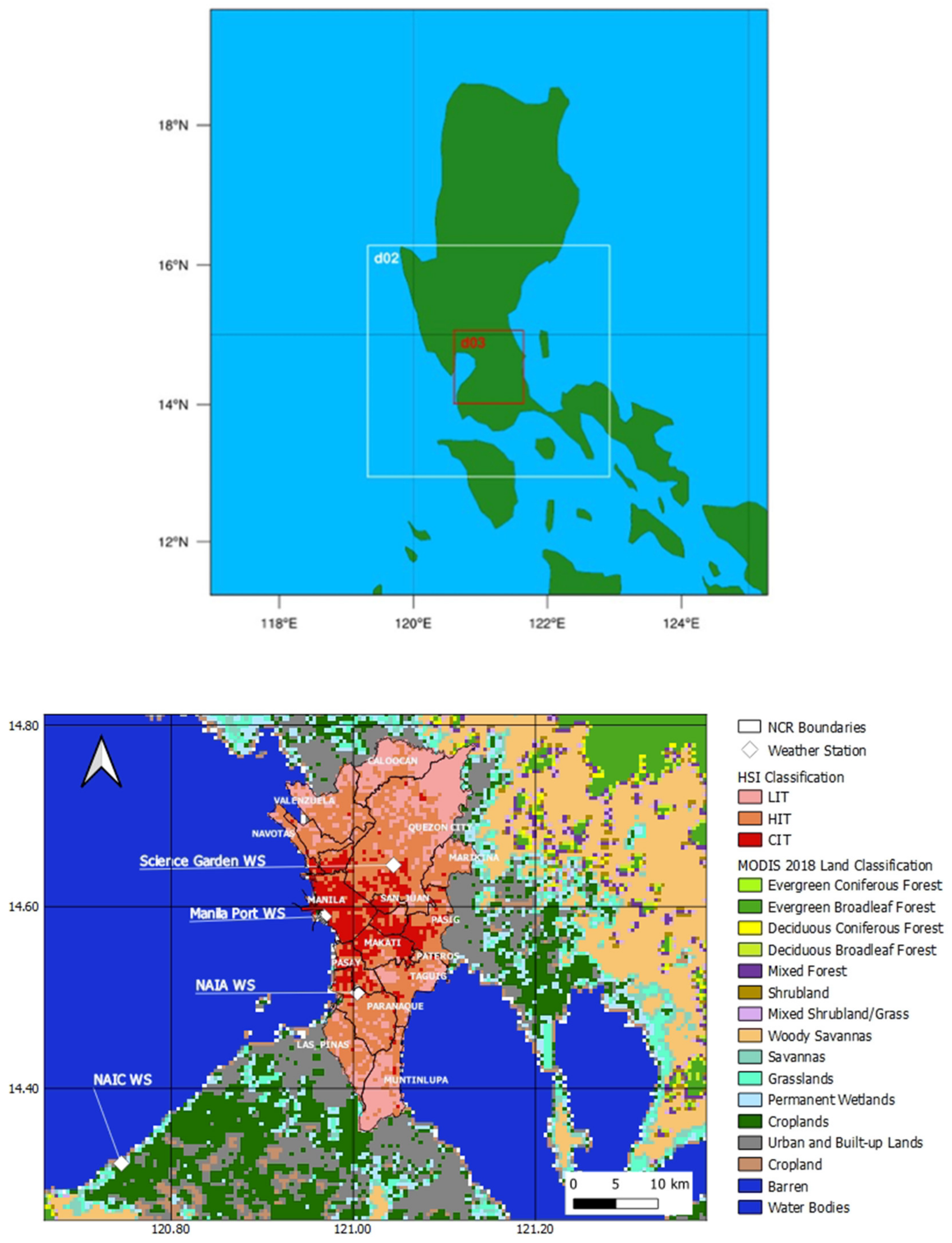
2.1. Study Area

Metro Manila is located at 14°35′ N, 121° E and covers an area of 636 km². It is located on an isthmus of two bodies of water, Manila Bay in the west and Laguna de Bay to the southeast, and is bounded by the Sierra Madre Mountain range to the east and northeast, and the Central Luzon plains to the north. Metro Manila is comprised of sixteen independent cities (one of which is Manila, the capital city of the Philippines), as well as an independent municipality. Each of these cities has its local government unit which gives them autonomy to create their land-use plan, with some cities having more built-up areas like Makati and Manila. These variations in land use may lead to differences in air and land surface temperature in the region. To simulate these spatiotemporal temperature variations, numerical models are used over a large area where urban features are parameterized. Furthermore, Metro Manila is composed of several cities and is divided into three districts, the Northern Manila District, Eastern Manila District, Southern Manila District, and Manila which is the capital district. The cities of Metro Manila are shown in Figure 1. In this study, Manila City is included in the Northern Manila District.

2.2. Meteorological Data

Data from NOAA’s Integrated Surface Dataset (ISD) in three meteorological stations in Metro Manila were used to validate WRF performance. ISD is a repository of worldwide surface weather observation from over 35,000 stations across the world (Smith, Neal, & Russ, 2011). The ISD data from Manila, Science Garden and NAIA was used. For comparison to rural air temperature, observation data from the BSWM Agromet station in Naic, Cavite was used. Naic is a first-class municipality of the province of Cavite and is located 47 km away from the city of Manila. MODIS land cover classifies Naic as a cropland area.

Table 1. Weather stations site information used in this study.

Observation Station	Location	Temporal Resolution	HSI/Land Use Category Location
Manila Port Area, Manila	14.59, 120.97	3-hourly	(3-Commercial/Industrial/Transportation)
Science Garden, Quezon City	14.65, 121.04	3-hourly	(2-High Intensity Residential)
NAIA, Pasay City	14.50, 121.00	hourly	(3-Commercial/Industrial/Transportation)
Naic, Cavite (Rural)	14.32, 120.75	hourly	Cropland

below shows the information of the observational stations including the HSI categories where the observations sites belong.

2.3. WRF Configuration

WRF v.3.9.1 [15] was used to simulate the near-surface variables in Metro Manila. WRF is a fully compressible, non-hydrostatic, mesoscale numerical weather prediction model that can also be used for urban studies application [31]. The model was configured with 3 one-way nested domains with a horizontal grid resolution of 9, 3, and 1 km and grid spacing of 100 × 105, 130 × 124, and 112 × 118, respectively, where the result from the innermost domain (d03) will be used in the analysis. The number of vertical layers is 40 sigma levels.

The initial and boundary condition used to drive the WRF model was taken from NCEP GDAS/FNL Operational Model Global reanalysis, which has a spatial resolution of 0.25° and a temporal resolution of 6 h [32].

WRF simulations were run from 0800 PHT on 21 April to 0000 PHT 30 April 2018, with an hourly resolution output. The first 16 simulated hours were treated as a spin-up period and discarded for simulation stability reasons, while the remaining hours constitutes the study period. The chosen study period coincides with the hot and dry season in Metro Manila. Furthermore, high temporals data sets were available from several stations for this period. A high heat index week was also forecasted during this period by the Philippine Atmospheric, Geophysical and Astronomical Services Administration (PAGASA), the country’s official weather bureau, and the highest air temperature and heat index recorded occurred on 25 April 2018 at 39.2 °C and 41 °C, respectively [33].

For the planetary boundary layer (PBL) parameterization, a Bougeault and Lacarrere scheme [34] was used since it supports the use of a multilevel urban canopy option. Other physical parameterizations used include Revised MM5 [35] for the surface layer, longwave and shortwave radiation for the RRTM [36] and Dudhia scheme [37] respectively. The land surface model is NOAH LSM [38] and Kain-Fritsch [39] for the cumulus parameterization.

Table 2. Configurations and physical parameterizations applied in WRF.

WRF Model	WRF V3.9
WRF Dynamical Solver	ARW
Domain Grid Spacing	D01: dx = 9000 m, dy = 9000 m D02: dx = 3000 m, dy = 3000 m D03: dx = 1000 m, dy = 1000 m
Land Use	MODIS 2018 data from LPDAAC data set with a spatial resolution of 30′.
Initial Meteorological Data	NCEP GDAS/FNL Operational Model Global Tropospheric Analyses Spatial Resolution = 0.25° Temporal Resolution = 6 h
Vertical Levels	40 with 16 levels below 1 km
	eta_levels =	1.000, 0.9986, 0.9972, 0.9958, 0.9943,
		0.9929, 0.9915, 0.9901, 0.9887, 0.9873,
		0.9859, 0.9845, 0.9824, 0.9792, 0.9749,
		0.9688, 0.9606, 0.9497, 0.9353, 0.9169,
		0.8935, 0.8646, 0.8296, 0.7884, 0.7412,
		0.6887, 0.632, 0.5724, 0.5115, 0.4506,
		0.3909, 0.3336, 0.2792, 0.2283, 0.1812,
		0.1379, 0.0984, 0.0599, 0.0279, 0.000
Physics Options	PBL: Boulac Scheme (BEP/BEM) Surface Layer: Revised MM5 Land Surface Model: NOAH LSM Longwave/Shortwave: RRTM/Dudhia Cumulus: Kain-Frisch (0 for d03) Microphysics: WRF Single Moment 3 (WSM3)

shows a summary of the physics scheme used for the simulation following earlier WRF studies in Philippine settings [29].

The modified Coronas climate classification places Metro Manila as a Type I climate which exhibits a distinct wet season from June to September, and a dry season for the rest of the year [40]. During the months of December, January, and February (DJF), Metro Manila experiences a distinct cool and dry season due to the cool air coming from the north. This season is known as the northeast monsoon, or locally known as “Amihan”. From March, April, and May (MAM), a transition period characterized by hot and dry winds is experienced due to the warm easterlies from the Pacific Ocean. Locally, this is considered as the summer season in the Philippines. The air temperature reaches its maximum during months of April and May [41], coinciding with period of this study. The months of June, July, and August (JJA) are characterized by hot and moist air and are considered as a wet or rainy season. The prevailing wind is the southwest monsoon or “Habagat”. Lastly, September, October, and November (SON) are also considered a transition period, where hot and wet winds originate from the West Philippine Sea. To add, higher tropical cyclone activities peaks during JJA and SON.

2.4. Updated Land-Use Data

WRF 3.9 and the recent version uses the default land-use classification from MODIS IGBP 21-category data. Although WRF allows usage of USGS land-use classification, both land-use data are outdated and may not reflect the rapid urban expansion since data were obtained from 1991 to 1992 [42]. One problem with the built-in land cover used by either USGS or MODIS is the homogeneity of urban land surfaces. In this study, land-use data will be updated into three urban subclasses given as an option by WRF—low-intensity residential (LIR), high-intensity residential (HIR), commercial/industrial/transportation (CIT). The human settlement index (HSI) will be used to subclassify the urban areas [43]. HSI uses a nighttime light image and the NDVI index to extract the residential site. HSI was used to extract urban areas where the nighttime light data was taken from the 2009 Defense Meteorological Satellite Program/Operational Linescan System (DMSP/OLS) [18]. One concern with the DMSP/OLS is the discontinuance of its operation after February 2014, which presents difficulty in urban extent extraction when performed after 2014. An alternative to this is the use of the Suomi National Polar-orbiting Partnership/Visible/Infrared Imaging Radiometer Suite (NPP/VIIRS), which was launched in 2011. The day-and-night band (DNB) area produced by VIIRS will be used to extract the three urban subcategories following the urban extent extraction study, using modified HSI by [18,44].

NDVI images were first generated from the monthly Landsat 8 OLI image for 2018 using Equation (1). Maximum NDVI is used from the multitemporal NDVI images to highlight urban areas. The use of NDVI poses concern as it has difficulty in distinguishing urban and bare lands, as well as water bodies, due to close index values [45]. To effectively differentiate urban areas from water bodies, NDWI is generated as a mask to remove the water bodies. NDWI is expressed using Equation (2).

$$NDVI=\frac{NIR-R}{NIR+R}$$

(1)

$$NDWI=\frac{G-NIR}{G+NIR}$$

(2)

where NIR, G, and R are the near-infrared, green, and red reflectance values from the Landsat8 OLI surface reflectance image.

To remove the cloud contamination, a composite NDVI was generated using the maximum algorithm. This is generated from multitemporal NDVI images and is expressed in Equation (3).

$$NDV{I}_{max}=MAX[NDV{I}_1,NDV{I}_2,NDV{I}_{3,\dots ,}NDV{I}_n]$$

(3)

To match the DN values of the NTL image and NDVI, first, zero-valued pixels were masked out and a natural logarithmic transformation was used to retain the details in the nighttime light. The data then were normalized using Equation (4) [46].

$$DN{B}_{ni}=\frac{DN{B}_i-DN{B}_{min}}{DN{B}_{max}-DN{B}_{min}}$$

(4)

where DNB_ni is the normalized value of the ith pixel, DNB_i is the original value of the ith pixel and DNB_min and DNB_max are the minimum and maximum values of all pixels.

HSI was calculated using Equation (5). The results were then used to classify urban lands into three subcategories. Pixels with HSI values of ≥80th percentile were classified as CIT areas, while HSI values between 30th and the 80th percentiles are classified as HIR areas, and HSI values of ≤ the 30th percentile are classified as LIR areas.

$$HSI=\frac{\left(1-NDVI\right)+DN{B}_{ni}}{\left(1-DN{B}_{ni}\right)+NDVI+DN{B}_{ni}\times NDVI}$$

(5)

HSI was only applied in Metro Manila. It was resampled to 500 m to match the spatial resolution of MODIS 15s 20-category LULC, which were used to classify land cover outside Metro Manila. MODIS data were retrieved from the Land Process Distributed Active Archive Center (LP DAAC) [47]. The HSI image of Metro Manila is shown in Figure 1. Upon observation, the three urban subclasses fit with the actual urban subclasses. For example, CIT coincides with the urban dense areas of Manila, Makati, Mandaluyong, Pasig, and some parts of Quezon City.

2.5. Experimental Design

Four experiments were performed in this study. First was the control simulation, designated as NO_URB (bulk), where urban parameters applied are based on NOAH LSM. Second was the integration of the single-layer UCM, designated as SLUCM, which integrates the urban canopy parameters of WRF but treats all urban areas as one category only (HIR). The third was the integration of building effect parameterization, designated as (BEP) and the fourth was the integration of building energy model to BEP, which is designated as BEM. Default values of urban parameters in the URBPARM.TBL were used in the simulation for Urban Canopy Model options due to the absence of urban morphology data in Metro Manila. It is important to note that this can be a source of uncertainty in the simulation.

2.6. Model Evaluation

To determine the performance of the model, the results of the simulations were assessed using performance statistics such as Mean Bias (MB), Root Mean Square Error (RMSE), Mean Absolute Error (MAE), and Index of Agreement (IOA) with Equations (6)–(9), respectively. The $y_i$ is the predicted value and $y_{i,obs}$ is the observed value.

$$MB=\frac{1}{N}{\displaystyle \sum }_{i=1}^N\left(y_i-y_{i,obs}\right)$$

(6)

$$RMSE=\sqrt{\frac{{{\displaystyle \sum }}_{i=1}^N{\left(y_i-y_{i,obs}\right)}^2}{N}}$$

(7)

$$MAE=\frac{1}{N}{\displaystyle \sum }_{i=1}^N\left(\left|y_i-y_{i,obs}\right|\right)$$

(8)

$$IOA=1-\frac{{{\displaystyle \sum }}_{i=1}^N{\left(y_i-y_{i,obs}\right)}^2}{{{\displaystyle \sum }}_{i=1}^N(\left|y_i-\overline{y}\right|+{\left|y_{i,obs}-\overline{y}\right|}^2)}$$

(9)

$$\overline{y}=\frac{1}{N}{{\displaystyle \sum }}_{i=1}^N{y}_{i,obs}$$

(10)

MB, RMSE, and MAE show the error or deviation of the modeled data from the observed data, while IOA shows how an error-free model predicts a variable.

Furthermore, the Nash-Sutcliffe efficiency coefficient (NSE) was also used to evaluate model performance and is expressed using Equation (11) [48]. NSE values can range from −∞ to 1, where the desired value should be close to 1 and negative values are regarded as unacceptable.

$$NSE=1-\frac{{{\displaystyle \sum }}_{i=1}^N{\left(y_i-y_{i,obs}\right)}^2}{{{\displaystyle \sum }}_{i=1}^N{\left(y_i-y_{mean}\right)}^2}$$

(11)

It is worth noting that in sensitivity studies, there are uncertainties in determining the threshold of values to determine if the model is performing well. In this study, the recommended values in

Table 3. Recommended values of statistical tests for the near surface variables adopted in this study.

Variable	Evaluation Parameter	Criteria
Temperature—2 m	RMSE MAE Mean Bias IOA	≤3.5 °C ≤2.0 °C ≤±2.0 °C ≥0.8
Relative Humidity—2 m	RMSE Mean Bias IOA	≤8.5% ≤±10.0% ≥0.60

, as adopted from the studies [49,50,51,52], will be used as a reference.

2.7. Calculation of Relative Humidity, Heat Index, and Relative Urban Heat Index

Relative humidity is not part of the measured output in ISD and WRF, hence it will be calculated as a function of temperature and dew point using the August–Roche–Magnus approximation [51] in Equation (12).

$$RH=100\frac{\exp \left(\frac{a{T}_D}{b+T_D}\right)}{\exp \left(\frac{aT}{b+T}\right)}$$

(12)

where T is the air temperature, T_D is the dew point temperatures, and the coefficients a = 17.67 and b = 243.5 [52].

Heat index (HI) is a measure of thermal comfort and is the temperature that a person feels given meteorological conditions. HI is calculated as a function of temperature and relative humidity, as is expressed using Equation (13) [53].

$$\begin{array}{cc}HI=-42.379& +2.04901523T_F+10.14333127RH-0.22475541T_{F}RH\hfill \\ & -6.83783\times {10}^{-3}{T}_F^2-5.481717\times {10}^{-3}{T}_F^{2}RH\hfill \\ & +1.22874\times {10}^{-3}{T}_F^{2}RH+8.5282\times {10}^{-4}TR{H}^2\hfill \\ & -1.99\times {10}^{-6}{T}^{2}R{H}^2 \hfill \end{array}$$

(13)

$T_F$ is the ambient dry bulb temperature in Fahrenheit and RH is the relative humidity in percentage.

The relative urban heat intensity is also simulated to determine the hot-spot and cold-spot in each region. Relative UHI is expressed using Equation (14), where D is the maximum absolute value of all UHI points in the area of interest [19]. The UHI is calculated as the difference in the air temperature with reference to an observed measurement located in a rural area (Naic, Cavite).

$$\begin{array}{c}Relative UHI \left(x,y\right)=\frac{UHI\left(x,y\right)}{D}\\ D=max\left|UHI\left(x,y\right)\right|\end{array}$$

(14)

Hotspots are those areas having positive relative UHI, while cold spots are those areas with negative relative UHI.

3. Results and Discussion

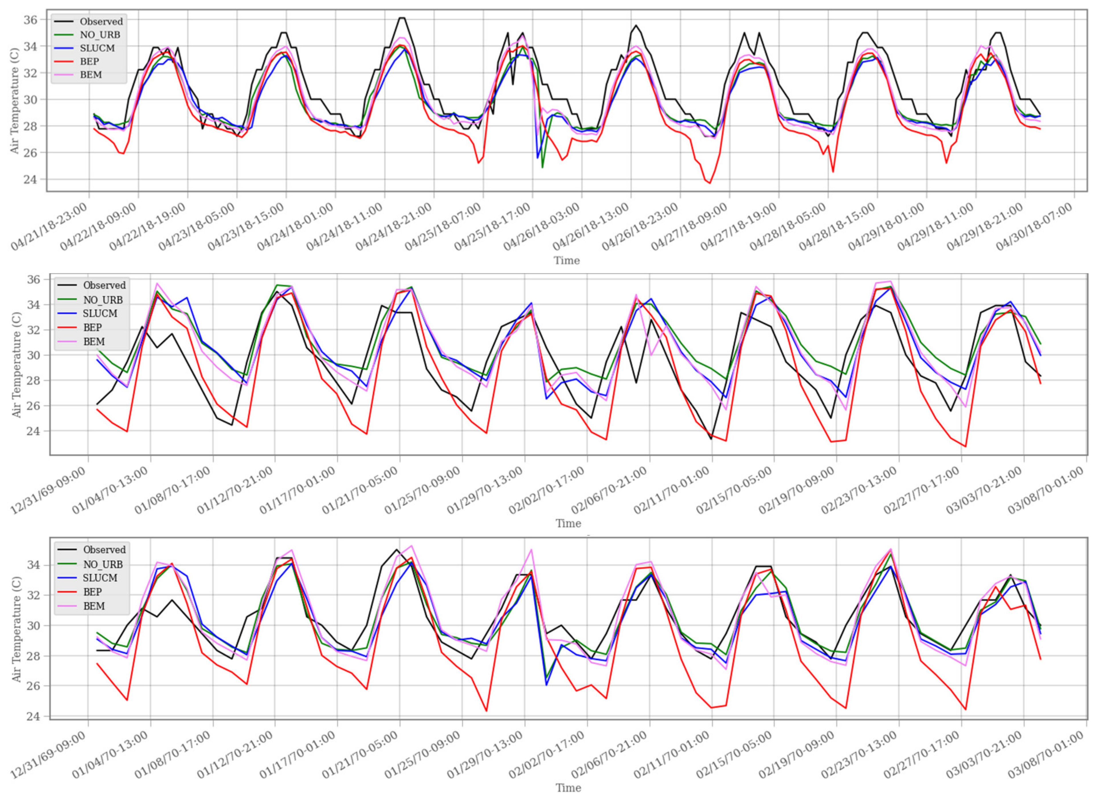
3.1. Comparison of Observed and Simulated Near-Surface Atmospheric Variables

3.1.1. 2 m Air Temperature

Table 4. Statistical performance result of no urban (NO_URB), single layer urban canopy model (SLUCM), building effect parameterization (BEP), and building energy model (BEM) over daily averaged air temperature for the three location sites.

Experimental Design	RMSE (°C)	MAE (°C)	Bias (°C)	IOA	NSE
NAIA, Pasay City
NO_URB	1.40	1.15	−0.91	0.90	0.69
SLUCM	1.56	1.30	−1.07	0.88	0.61
BEP	1.80	1.59	−1.50	0.89	0.48
BEM	1.21	0.99	−0.79	0.94	0.76
Manila Port Area, Manila
NO_URB	0.98	0.68	−0.09	0.94	0.76
SLUCM	1.13	0.82	−0.33	0.92	0.68
BEP	2.09	1.72	−1.28	0.84	−0.11
BEM	1.31	0.97	−0.24	0.91	0.57
Science Garden, Quezon City
NO_URB	2.46	1.95	1.56	0.79	0.35
SLUCM	2.06	1.67	1.01	0.86	0.52
BEP	2.41	1.84	−0.82	0.88	0.35
BEM	2.10	1.73	0.91	0.86	0.50

shows the statistical result for the air temperature, with bold fonts showing the best result. The RMSE and MAE values for NAIA and Manila Port show good agreement where values are ≤3 °C and ≤2 °C, respectively; these are within the recommended values as discussed in Section 2.6, except for Science Garden station (SGQ). The air temperature is generally underestimated in NAIA and Manila Port, which are in the CIT region, while overestimation is observed in HIR region where SGQ is located. A high IOA (around 0.80 and higher) is observed for all sites and experiments. NSE mostly shows positive values, indicating good performance of the model. Although all designs are within the benchmark values, results indicate that there is no single design that shows the best performance for all sites. For example, BEM works best for NAIA, while the NO_URB works for Manila Port and SLUCM for SGQ. The expectation was the MUCM should generally perform well compared to NO_URB and SLUCM because MUCM considers urban morphology and energy parameters. However, the results showed otherwise where BEP has the highest errors. This observation was similar to [54], where results showed simpler models performing as effective as the complex models.

One probable reason for this is the PBL option used for the MUCM. Currently, WRF-MUCM supports the use of MYJ and BOULAC only, while former WRF study used in Metro Manila recommends the use of Yonsei University Scheme (YSU) [41]. The integration of YSU into MUCM would greatly enhance the near-surface atmospheric variables. On the other hand, the biases observed may be mainly due to the inaccurate simulation of the surface layer energy budget. For example, underestimation of surface air temperature was potentially attributed to the underestimation of the absorbed solar shortwave radiation and the upward surface sensible heat flux [42]. On the other hand, overestimation was attributed to the underestimation of the outgoing longwave radiation or the overestimation of the upward surface flux [16]. Moreover, the inaccurate representation of the urban morphology may also contribute to the biases observed as urban morphology affects the radiation processes and energy balance in an urban area. The default WRF urban parameters used may not be reflective of the actual urban conditions in Metro Manila. This is similar to a study done by Sun et al. [55], where they found that WRF urban parameters tend to distort the morphology of Chinese cities, significantly affecting the surface energy balance process and leading to inaccurate surface temperature simulation. Other studies noted accurate urban surface representations and parameters are needed to accurately simulate temperature variation in an urban area [56,57,58,59]. For example, detailed information of the urban morphology and high-resolution urban canopy parameters are needed to correctly quantify anthropogenic heat, which affects accurate air temperature simulation [60]. Currently, no available studies or data have been conducted to determine the Philippines urban morphology that can be used for WRF in urban simulation. Hence, updating WRF urban parameters for the Philippines setting would further enhance the performance of the model. Furthermore, absence of surface energy balance measurements restricted researchers from further characterizing the air temperature. But for the purpose of this study, the BEM model performs reasonably well as it is within the recommended values used in this study. The temporal evolution of air temperature was also analyzed to determine if the simulations can follow the observed trend.

Figure 2 shows that the model performs relatively well, as evidenced by the simulated trends being close to the observed trend. NAIA generally underestimated the air temperature, while Manila Port and SGQ overestimated the air temperature during daytime but underestimated it at nighttime. Furthermore, with the current WRF set-up, all experiments were unable to accurately simulate the air temperature as they either underestimated or overestimated it. NAIA had a lower range of air temperature, although the minimum temperature was around 28 °C, while SGQ had the lowest minimum temperature averaging at 25 °C. It is interesting to note than an improvement in the air temperature trend is seen when using BEP and BEM during daytime, especially when the air temperature is at its peak during afternoon.

The time series of the Sensible Heat Flux or SHF seen in Figure A1 was also checked, since in a study it was found out that it directly affects surface temperature [61]. BEM showed the highest peak of SHF during afternoon and BEP with the lowest SHF during nighttime similar to Figure 2. This suggests that the high peak air temperature simulated by BEM in the afternoon and the low air temperature simulated by BEP in the evening is directly influenced by the simulated SHF. Furthermore, other studies have shown BEP unable to simulate nighttime temperature accurately. A modification to the BEP by adding an anthropogenic heat flux terms was proposed to address this [62].

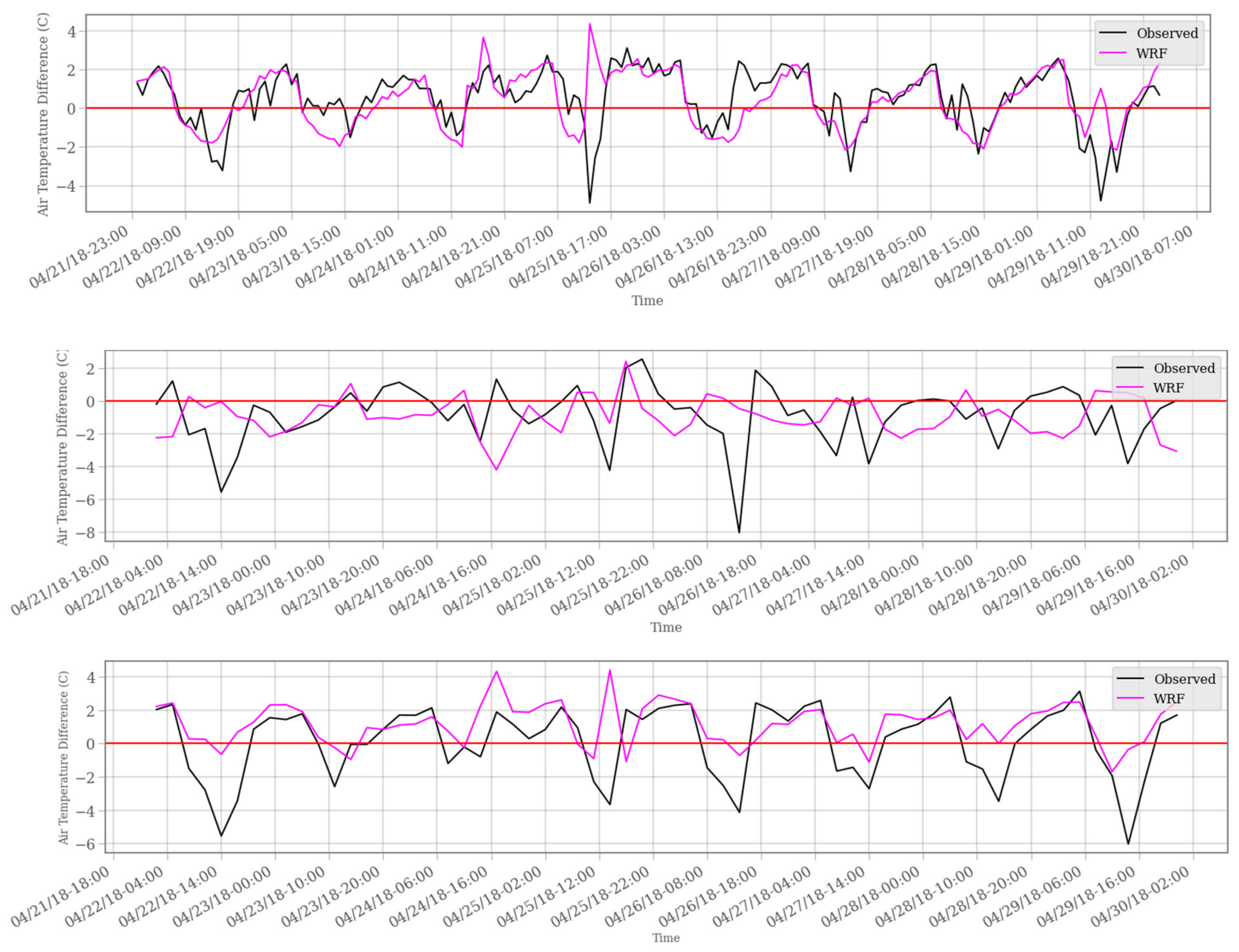
3.1.2. Diurnal Variation of Air Temperature

Urban heat island is primarily characterized by high temperature at nighttime; hence, a validation study was conducted where the 2 m air temperature was aggregated into daytime (7:00–17:00) and nighttime (18:00–6:00) to determine if the model can simulate well the diurnal pattern of the 2 m air temperature.

Results vary depending on the experiment and location, as seen in

Table 5. As in Table 4 but for the diurnal air temperature. D refers to daytime and N to nighttime.

Experimental Design	RMSE (°C)		MAE (°C)		Bias (°C)		IOA		NSE
	D	N	D	N	D	N	D	N	D	N
			NAIA, Pasay City
NO_URB	1.57	1.23	1.43	0.91	1.57	−0.56	0.82	0.73	0.23	0.29
SLUCM	1.80	1.30	1.67	0.89	1.80	−0.64	0.78	0.73	−0.01	0.20
BEP	1.68	1.88	1.52	1.64	1.68	−1.62	0.83	0.68	0.12	−0.67
BEM	1.27	1.14	1.12	0.88	1.29	−0.75	0.88	0.80	0.48	0.38
			Manila Port Area, Manila
NO_URB	1.08	0.87	0.83	0.53	−0.16	−0.01	0.91	0.81	0.59	0.31
SLUCM	1.33	0.90	1.03	0.61	−0.44	−0.22	0.87	0.83	0.38	0.26
BEP	2.08	2.11	1.51	1.93	−0.63	−1.93	0.80	0.58	−0.52	−3.1
BEM	1.73	0.67	1.37	0.57	−0.20	−0.27	0.82	0.91	−0.05	0.58
			Science Garden, Quezon City
NO_URB	1.99	2.84	1.28	2.63	0.65	2.46	0.79	0.57	−0.01	−1.26
SLUCM	1.82	2.28	1.36	1.98	0.21	1.81	0.83	0.66	0.17	−0.45
BEP	2.98	1.64	2.30	1.37	−0.60	−1.03	0.73	0.85	−1.24	0.25
BEM	2.12	2.09	1.62	1.85	0.16	1.67	0.81	0.69	−0.13	−0.22

. SGQ yielded the highest RMSE and MAE of greater than 2 °C for both day and night, while Manila had the lowest RMSE and MAE of less than 2 °C. In terms of Bias, the result shows underestimation for NAIA and Manila Port, while overestimation is observed for SGQ. NO_URB performed best for Manila Port and BEM for NAIA, while varying results are observed for SGQ. In most cases for both daytime and nighttime, BEP registered the highest errors and lowest correlation in all sites. A more realistic and site-specific urban morphology and parameters as opposed to using the default WRF parameters may improve the daytime and nighttime 2 m air temperature simulation, as suggested by Segura et al. [21]. On the other hand, it is interesting to note the addition of the anthropogenic heat offsets the errors of BEP as seen in the BEM simulations. This is because BEM considers latent and sensible anthropogenic heat in the 2 m air temperature simulation. Furthermore, it was suggested that improvement of the solar radiation simulation or soil moisture may improve the biases of BEP simulation. Overall, result shows no single experiment that is best for all sites.

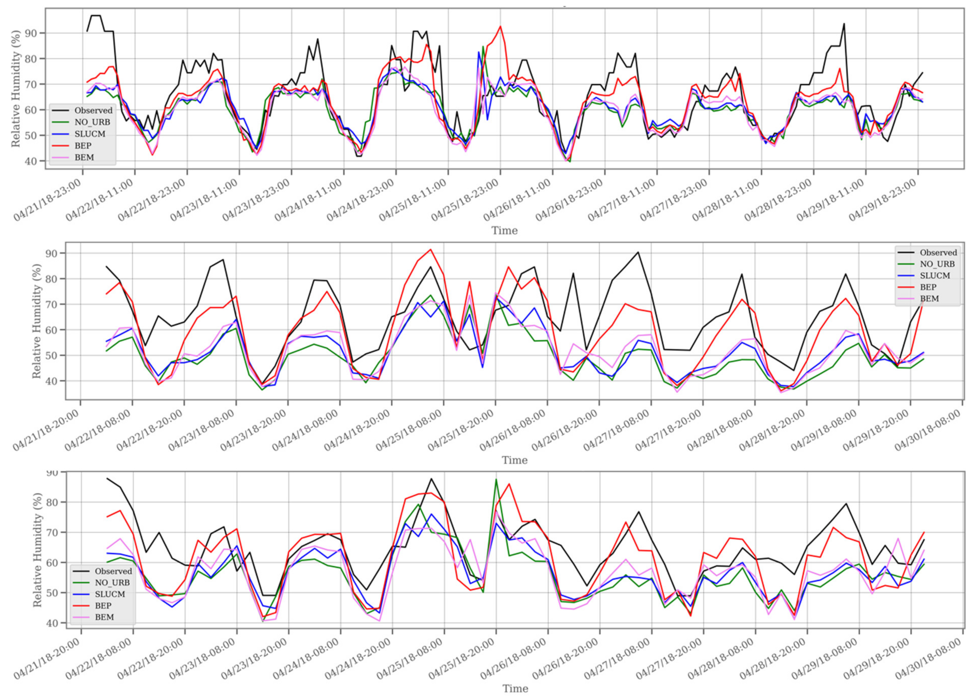
3.1.3. Relative Humidity

Table 6. As in Table 4 but for relative humidity.

Experimental Design	RMSE (%)	MAE (%)	Bias (%)	IOA	NSE
NAIA, Pasay City
NO_URB	10.3	7.55	−5.13	0.75	0.35
SLUCM	10.0	7.22	−4.24	0.75	0.40
BEP	8.46	6.13	−2.21	0.86	0.57
BEM	9.82	7.02	−5.35	0.80	0.42
Manila Port Area, Manila
NO_URB	11.7	9.96	−9.03	0.66	−0.68
SLUCM	10.7	8.90	−8.28	0.68	−0.41
BEP	8.57	6.87	−3.40	0.82	0.10
BEM	10.9	9.22	−7.91	0.68	−0.45
Science Garden, Quezon City
NO_URB	19.2	16.1	−15.3	0.56	−1.23
SLUCM	17.2	14.0	−13.4	0.60	−0.80
BEP	11.3	8.86	−5.23	0.82	0.22
BEM	16.6	13.8	−12.7	0.62	−0.67

shows the statistical performance of relative humidity. Underestimation is generally observed in all sites and designs. The highest underestimation was observed in SGQ-NO_URB, at 15.30% while NAIA- BEP showed the least at 2.213%. RMSE and MAE were lowest for NAIA at 8.461% and 6.134%, respectively, while SGQ had the highest at 19.17% and 16.05%, respectively. The simulation shows high agreement between model and observation, with IOA greater than 0.5, while NSE shows varying values depending on the site, which can be attributed to the size of the observations.

Results show that the addition of MUCM improved the performance of all statistical tests. Specifically, BEP performed best for all sites while the NO_URB gave poor results. Although improvement was observed with the addition of BEP, all designs did not meet the recommended values. Difficulty in simulating RH can be based on many factors, such as the soil moisture initialization and the land surface model in WRF [63]. Figure 3 shows the temporal evolution of the observed and simulated relative humidity. Result showed that the models can capture the observed trend, although underestimation was observed in all sites consistent with the result in Table 6. BEP showed good performance in all sites, while NO_URB performed poorly. Higher relative humidity was observed during nighttime, but it decreased as it approached daytime especially during the afternoon. All experiments seem to fail to capture the high peaks during nighttime, while at daytime, NAIA can capture the low peaks. PORT and SGQ do not show the same trend, which can be a result of its low temporal resolution.

3.2. Urban Heat Island Intensity (UHII)

To estimate the intensity of urban heat in Metro Manila, the difference in the air temperature of the observed sites and in Naic, Cavite was taken. Figure 4. shows the observed and WRF simulated UHII. Positive UHII indicates higher air temperature in the urban area, while negative UHII indicates higher air temperature in the rural area.

Generally, results show that WRF can simulate the observed UHII trend, although overestimations are observed. For the Naic-NAIA, the maximum UHII trend were mostly observed during nighttime, which indicates the presence of UHI. This is also observed in Manila, where higher air temperature difference was observed during nighttime. But, the case for SGQ is different where higher air temperature were mostly observed during daytime, similar to the study by Manalo et al. [64]. This can probably be attributed to the fact that SGQ (HIR category) has a relatively higher greenery compared to the other two sites (CIT category). It is interesting to note that negative UHI is mostly observed in urban areas during daytime which may suggest that features and materials in urban environments have an overall cooling effect [59]. This is also observed in other studies where they termed this condition as urban cooling island (UCI), opposite of UHI [65,66]. The negative UHIs observed can be a result of the differing heat capacities in rural and urban areas where the former is more exposed to solar radiation during daytime, resulting in faster heating compared to urban areas [64,67]. Another reason ia the shading effect from buildings in urban areas [68,69,70], which lower temperatures. The shading effect is taken into account in WRF UCM simulations [31]. Generally, the diurnal trend goes from high rural temperature during daytime and peaks at noon resulting to UCI in urban areas, while higher urban temperature is predominantly observed during nighttime as a result of UHI. Maximum observed nighttime air temperature difference is noted at 3 °C on 26 April 2018 in NAIA, while the minimum observed daytime air temperature difference in rural areas is at −8 °C on 26 April 2018 in SGQ.

The average relative UHI for the entire study period in Metro Manila, which shows the spatial distribution of UHI, is shown in Figure 5. At 08:00, hot spots were already observed in the Port Area of Manila and the areas near Laguna Lake, which includes the cities of Muntinlupa and Taguig after values reaching up to 0.30. On the other hand, prominent cold spots were observed in the area north of Quezon City, where the La Mesa watershed is located, and the inner part of the cities of Las Piñas and Parañaque. It is interesting to note that the hot spots observed were near open waters. This suggests these areas are either vegetated or have less urban build-up, which resulted in the observed cold spots. At 14:00, the previous hotspots observed near Laguna Lake evolved into a high cold spot. This included the southern Metro Manila areas, where values reach up to −1.0. On the other hand, Manila and its surrounding cities remained as hotspots having a higher positive relative UHI where values reach up to 0.70. Cold spots were found in the areas of Mandaluyong, Makati, and Taguig despite having dense built-up structures, probably because of building shade, which reduces solar exposure. At 20:00, it is interesting to note that most of Metro Manila experience hotspots, which is indicative of the urban heat island phenomenon. High, positive relative UHIs are specifically observed in northern and central Metro Manila. Specifically, the cities of Manila, Valenzuela, Caloocan, and Navotas, and the areas near Laguna Lake in the cities of Taguig and Muntinlupa, show high UHI.

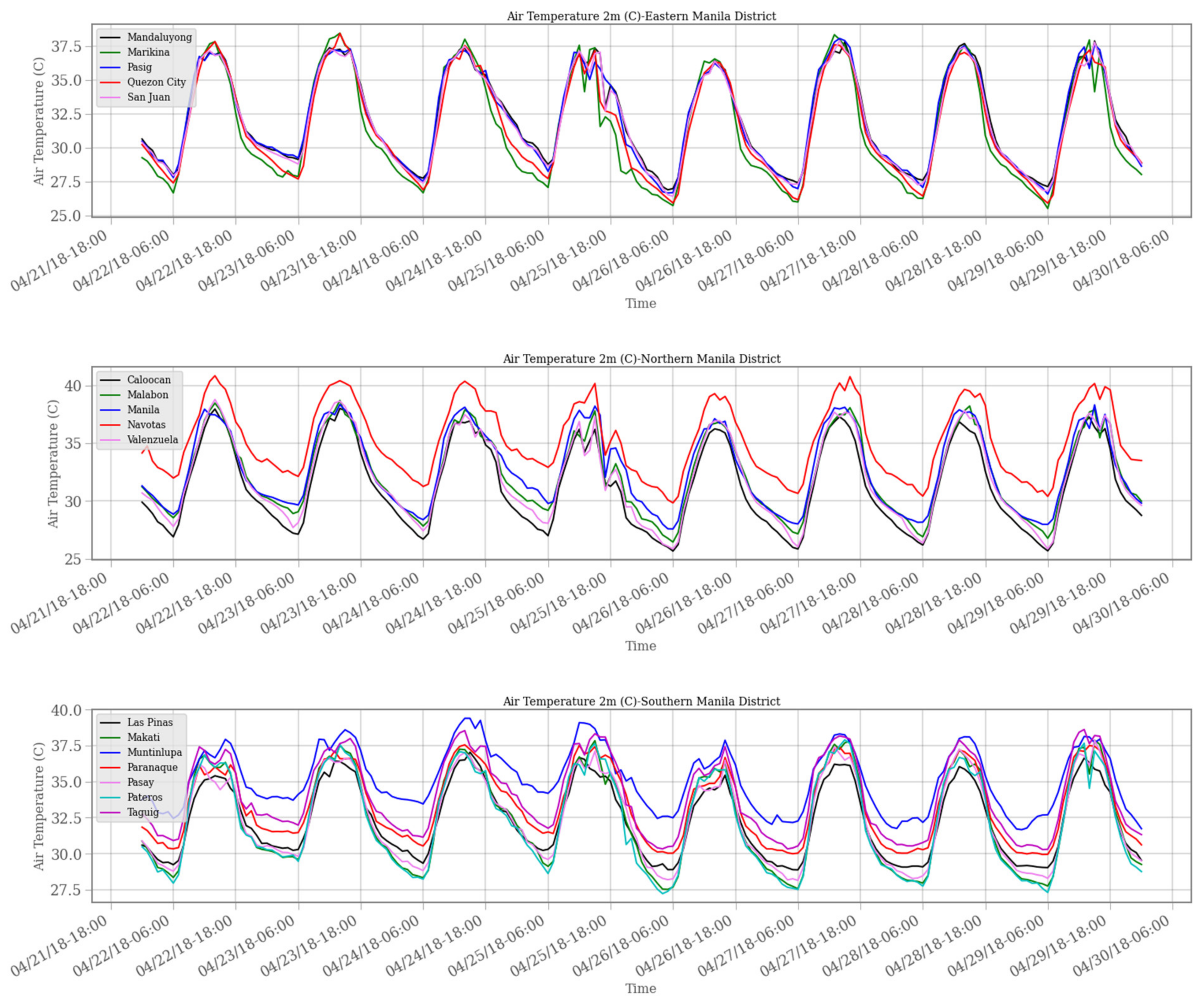
3.3. Air Temperature by Administrative District

As previously discussed, Metro Manila is an urban conurbation comprised of 16 independent cities and one independent municipality each having its autonomy in implementing a land-use development plan. Because of this, variations in land use may lead to a variation of urban heat intensity. In this regard, the study seeks to determine, which cities have the highest urban heat. This would help the local government units in assessing and creating plans to mitigate and urban heat.

Figure 6 shows the average time series air temperature for the three administrative districts in Metro Manila using zonal statistics. A larger range of air temperature is observed in Northern Manila District (NMD) while Southern Manila District (SMD) has the smallest range. It is interesting to note that SMD has the lowest air temperature peak, which does not reach 35 °C, when compared to the other two districts. In terms of intercity temperature variation, Eastern Manila District (EMD) has the lowest average standard deviation at 0.22, while NMD has the highest at 0.42. However, at nighttime, SMD shows a lower average standard deviation at 0.21, while NMD has the highest at 0.59.

On average, NMD has the highest air temperature at 31.04 °C, SMD has the lowest air temperature at 30.11 °C. By city component, Muntinlupa has the lowest average day and night air temperatures at 30.50 °C and 27.74 °C, respectively, while Navotas shows the highest at 32.7 °C and 29.49 °C, respectively.

Considering the location of SMD, which is near Laguna Lake, urban–lake breeze interaction may have a significant effect on the observed lower air temperature range. Pressure differences between lake and land cause the air in the urban area to rise up and be displaced by the cool air from the lake [71]. This vertical transport results in cooler near-surface air, which explains a relatively low air temperature in SMD. Although, the opposite is observed during nighttime in areas near the lake. During nighttime, it can be observed that although SMD shows low nighttime air temperature range, a slower dissipation rate of heat as the night progresses is seen in the air temperature dips. NMD and EMD shows minimum air temperature reaching below 26 °C, while SMD only reaches slightly below 27 °C. This is observed at 5 to 6 in the morning. Mean nighttime air temperature taken at 5:00 gives SMD the highest average temperature at 27.59 °C, while 27.41 °C and 27.35 °C was recorded for NMD and EMD, respectively. This is of interest considering SMD is near Laguna Lake and should have a lower air temperature. This occurrence was also observed in a simulation where it was noted that the cooling effect of the lake weakens and starts to warm up its surroundings, peaking early in the morning [72]. It was concluded that water temperature dictates the temperature change where water bodies, after reaching a higher temperature than its surrounding areas, act as nocturnal warming elements. This occurrence is usually observed during hot season.

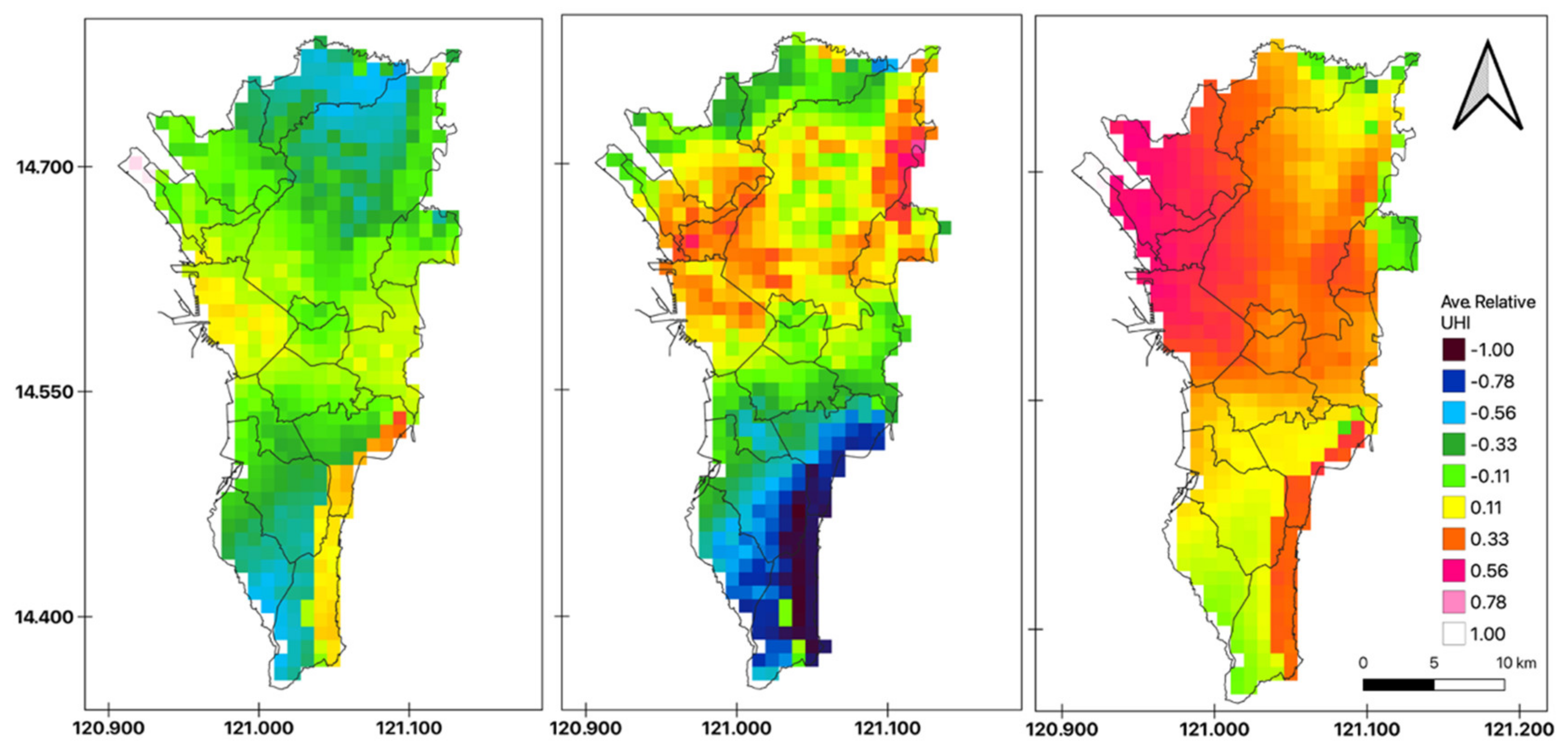
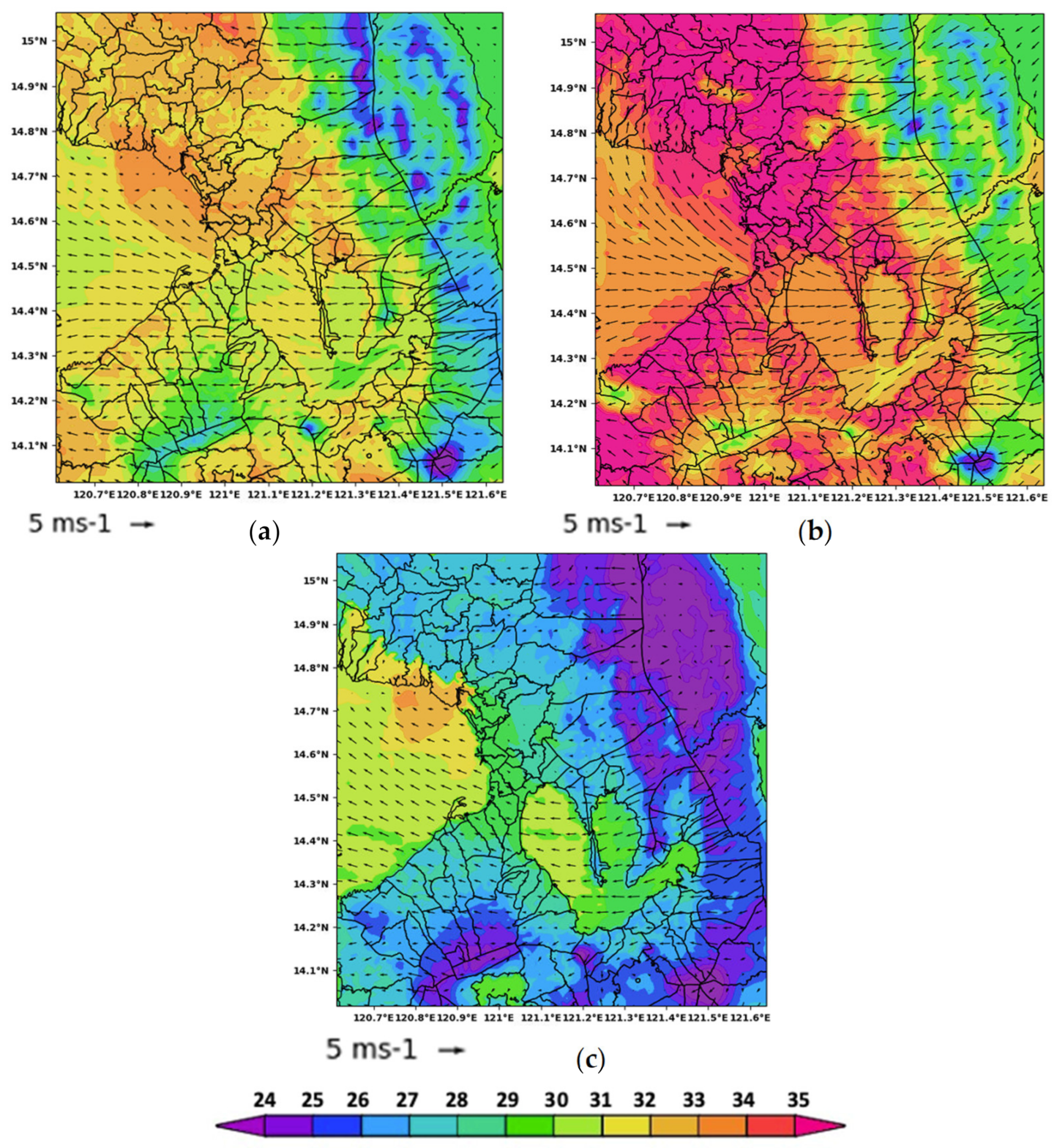
3.4. Spatial Variation of Air Temperature in Metro Manila

The results discussed in Section 3.3 show the average air temperature for the entire grid cell per city. They do not show the air temperature variation for the entire region. To better represent the variations, a spatial map of the average air temperature overlaid with the 10 m winds of Metro Manila is shown in Figure 7. The BEM simulation is used to generate the map to take into consideration effects of urban morphology. Further, results for BEM for air temperature are within the acceptable range. The map for 9:00, 14:00, and 20:00 is presented to show how air temperature, wind speed, and wind direction evolved for the day.

High air temperature at around 32–33 °C is observed at 9:00 in northern parts of Metro Manila, the central part of Quezon City, Marikina, Pasig, and San Juan. These areas have dense urban build-up, which explains their high air temperature. Furthermore, stagnant winds are also observed in the said areas, which may contribute to the high air temperature. The effect of stagnant wind with air temperature is further discussed in the next section.

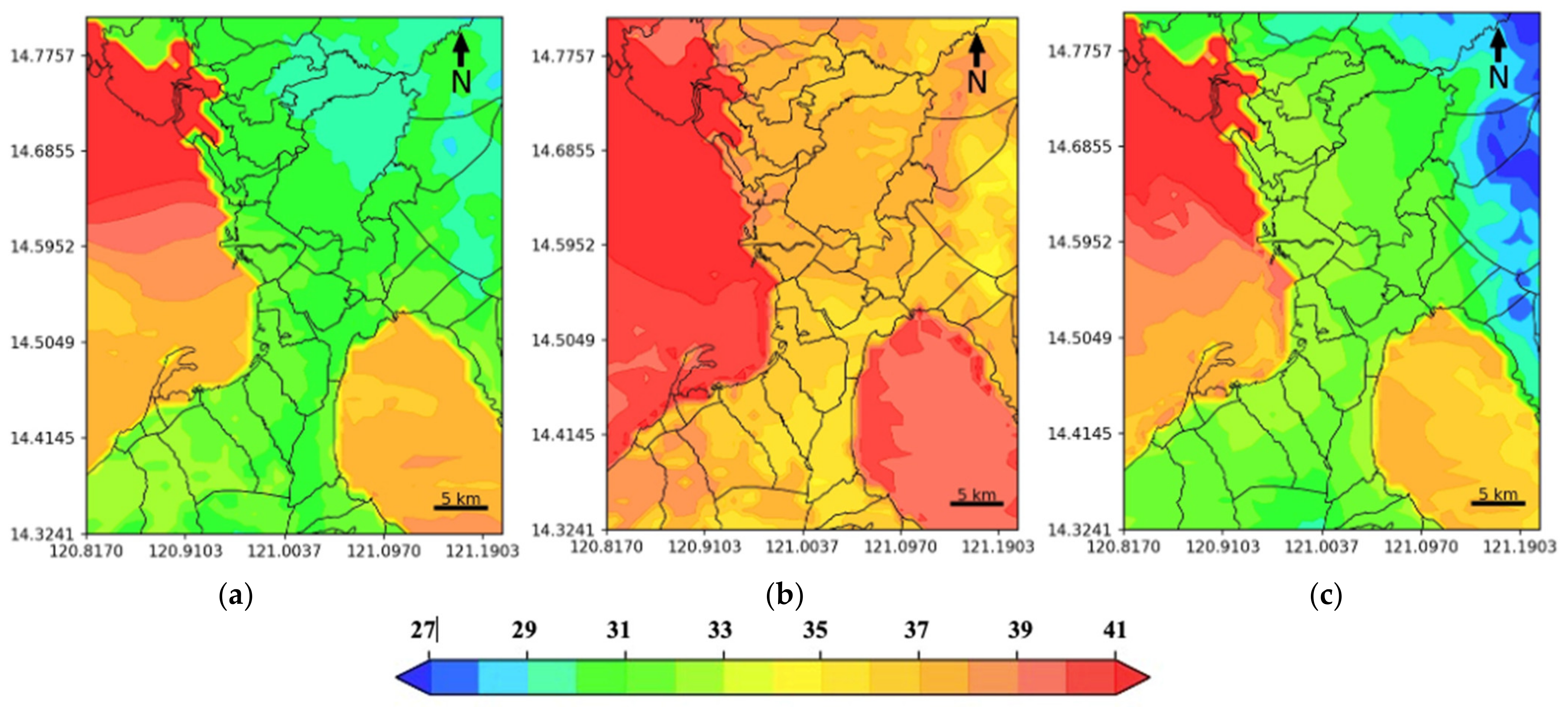
3.5. Spatial Variation of Heat Index in Metro Manila

Generally, PAGASA reports the HI based on the observations from the synoptic weather station. This, however, does not represent the spatial variation of HI canopy in terms of thermal comfort [19]. Numerical simulations like WRF can produce continuous spatial distribution, which can be used to assess the thermal comfort.

Figure 8 shows the distribution of the averaged HI in Metro Manila for daytime and nighttime. High HI of 35 °C is immediately observed at 8:00 in the cities of Manila, Pasay, Makati, and Mandaluyong. On the other hand, cities in southern Metro Manila and the areas northeast of Quezon have a lower HI at 32–33 °C. At 14:00, HI evolved to cover almost the entire Metro Manila at greater than 36 °C while cities near Laguna Lake remained at 34 °C. At nighttime, high HI at 31–34 °C is still observed in most part of the region, although cities near the Sierra Madre range have lower HI compared to those that are further away.

Consistent high HI is observed in open waters and areas near to them, especially the northwestern part of Metro Manila. As an example, daytime and nighttime average HI for Muntinlupa, Taguig, and Navotas, which are near open waters, are over 36 °C and 33 °C, respectively, whereas other cities are lower by around 1–2 °C. Open water tends to increase the humidity, resulting in an increase of HI in its surrounding areas. This was also observed by where open water bodies increase the humidity, dampening the positive effects on thermal comfort.

Overall, Navotas had the highest averaged HI throughout the study duration at 35 °C, while Marikina had the lowest at 31 °C. In terms of HI classification, result shows thermal discomfort for Metro Manila during the entire day. During daytime, HI is classified as Extreme Caution for the entire Metro Manila, while at nighttime it is classified as Caution.

4. Conclusions

The present study investigates the performance of WRF in simulating the air temperature and relative humidity in Metro Manila. Sensitivity analyses were conducted to determine the effectiveness of using the urban canopy model (UCM) options in WRF. Using the VIIRS nightlight image and the Human Settlement Index, Metro Manila was categorized into three suburban categories to take into consideration the effects of urban morphologies for the multilevel UCM.

The results show that the addition of UCM does not necessarily improve the performance of WRF in simulating near-surface meteorological variables. For example, simulation of air temperature shows that improvement using UCM is site dependent. Nighttime air temperature is better simulated by WRF compared to daytime. On the other hand, simulation of relative humidity still presents a challenge. Although, the use of UCM somehow improved the relative humidity simulation. The use of appropriate planetary boundary layers and contextualized urban parameters may improve the simulations. In this study, the default urban parameters used may not reflect the actual urban conditions of Metro Manila. Hence, a separate study can be conducted to locally contextualized the urban parameters in Metro Manila using the local climate zone (LCZ) classification [73], which can be integrated into WRF. Moreover, the use of another LSM such as NOAH-MP is shown to improve the simulation of near-surface meteorological variables [25]. Furthermore, important surface processes may not have been properly represented by WRF such as local land breeze/sea breeze, which is important for local wind simulations. This can be explored in another study.

UHII simulation shows hotspots in Metro Manila, especially during nighttime, indicating the presence of urban heat island. U HII values reached to a maximum of 3 °C higher during nighttime and 8 °C higher during daytime in Metro Manila. The presence of water bodies significantly reduces the air temperature of surrounding areas. This is observed where SMD has a lower air temperature compared to NMD and EMD, since it is located near Laguna Lake. Although, during nighttime, SMD is observed to have a higher air temperature due to Laguna Lake acting as a heat source during the hot season. Although air temperature is relatively lower in areas near water bodies, the heat index was observed to be high in these areas due to higher relative humidity. Generally, Metro Manila experiences thermal discomfort throughout the day until nighttime. The high HI at nighttime posits a concern especially for the physiologically vulnerable population who does not have any access to air conditioning facilities, which is relevant to Metro Manila due to the possible effects of heat stress.

The results from this study may be used by the local government as baseline data for projects and policy recommendations in reducing urban heat. Future works would focus on using WRF to simulate different mitigation strategies to reduce urban air temperature such as simulation of cool roof [74] or green spaces [75]. Furthermore, a study of a localized anthropogenic heat source is recommended, which can then be integrated into WRF to determine the contribution of human activities to urban heat in Metro Manila.

References

1. UN-HABITAT. The State of the World’s Cities 2008-2009: Harmonious Cities; United Nation Centre for Human Settlements: Nairobi, Kenya, 2010; ISBN 978-92-1-132010-7. [Google Scholar]
2. Navarro, A. Scrutinizing Urbanization Challenges in the Philippines through the Infrastructure Lens; Philippine Institute for Development Studies: Manila, Philippines, 2014. [Google Scholar]
3. Angel, S.; Blei, A.; Lason-Hall, P.; Sanchez, N.G.; Gopalan, P.; Kallergis, A.; Civco, D.; Kumar, S.; Madrid, M.; Shingade, S.; et al. Atlas of Urban Expansion. Available online: http://atlasofurbanexpansion.org/cities/view/Manila. (accessed on 12 March 2020).
4. Friedmann, J.; Sorensen, A. City Unbound: Emerging Mega-Conurbations in Asia. Int. Plan. Stud. 2019, 24, 1–12. [Google Scholar] [CrossRef] [Green Version]
5. Oke, T. The Heat Island of the Urban Boundary Layer: Characteristics, Causes and Effects. NATO ASI Ser. E Appl. Sci. -Adv. Study Inst. 1995, 277, 81–108. [Google Scholar] [CrossRef]
6. Wang, W.; Liu, K.; Tang, R.; Wang, S. Remote Sensing Image-Based Analysis of the Urban Heat Island Effect in Shenzhen, China. Phys. Chem. Earth Parts A/B/C 2019, 110, 168–175. [Google Scholar] [CrossRef]
7. Keeratikasikorn, C.; Bonafoni, S. Urban Heat Island Analysis over the Land Use Zoning Plan of Bangkok by Means of Landsat 8 Imagery. Remote Sens. 2018, 10, 440. [Google Scholar] [CrossRef]
8. Tiangco, M.; Lagmay, A.M.F.; Argete, J. ASTER-Based Study of the Night-Time Urban Heat Island Effect in Metro Manila. Int. J. Remote Sens. 2008, 29, 2799–2818. [Google Scholar] [CrossRef]
9. Firozjaei, M.K.; Weng, Q.; Zhao, C.; Kiavarz, M.; Lu, L.; Alavipanah, S.K. Surface Anthropogenic Heat Islands in Six Megacities: An Assessment Based on a Triple-Source Surface Energy Balance Model. Remote Sens. Environ. 2020, 242, 111751. [Google Scholar] [CrossRef]
10. Wang, X.; Huang, G.; Lin, Q.; Nie, X.; Liu, J. High-Resolution Temperature and Precipitation Projections over Ontario, Canada: A Coupled Dynamical-Statistical Approach. Q. J. R. Meteorol. Soc. 2014, 141, 1137–1146. [Google Scholar] [CrossRef]
11. Wolters, D.; Brandsma, T. Estimating the Urban Heat Island in Residential Areas in the Netherlands Using Observations by Weather Amateurs. J. Appl. Meteorol. Climatol. 2012, 51, 711–721. [Google Scholar] [CrossRef]
12. Manalo, J.A.; Matsumoto, J.; Takahashi, H.G.; Villafuerte, M.Q.; Olaguera, L.M.P.; Ren, G.; Cinco, T.A. The Effect of Urbanization on Temperature Indices in the Philippines. Int. J. Climatol. 2021, 1–18. [Google Scholar] [CrossRef]
13. Hidayat, D.J.; Soekirno, S. Development of Temperature Monitoring and Prediction System for Urban Heat Island (UHI) Based on the Internet of Things. J. Phys. Conf. Ser. 2021, 1816, 12054. [Google Scholar] [CrossRef]
14. Oh, J.W.; Ngarambe, J.; Duhirwe, P.N.; Yun, G.Y.; Santamouris, M. Using Deep-Learning to Forecast the Magnitude and Characteristics of Urban Heat Island in Seoul Korea. Sci. Rep. 2020, 10, 3559. [Google Scholar] [CrossRef] [Green Version]
15. Skamarock, W.; Klemp, J.; Dudhia, J.; Gill, D.; Barker, D.; Duda, M.; Huang, X.; Wang, W. A Description of the Advanced Research WRF Version 3; University Corporation for Atmospheric Research: Boulder, CO, USA, 2008. [Google Scholar]
16. Giannaros, T.M.; Melas, D.; Daglis, I.A. Numerical Study of the Urban Heat Island over Athens (Greece) with the WRF Model. Atmos. Environ. 2013, 73, 103–111. [Google Scholar] [CrossRef]
17. Fallmann, J.; Emeis, S.; Suppan, P. Mitigation of Urban Heat Stress—A Modelling Case Study for the Area of Stuttgart. Erde 2013, 144, 202–216. [Google Scholar] [CrossRef]
18. Chen, F.; Yang, X.; Zhu, W. WRF Simulations of Urban Heat Island under Hot-Weather Synoptic Conditions: The Case Study of Hangzhou City, China. Atmos. Res. 2014, 138, 364–377. [Google Scholar] [CrossRef]
19. Bhati, S.; Mohan, M. WRF Model Evaluation for the Urban Heat Island Assessment under Varying Land Use/Land Cover and Reference Site Conditions. Theor. Appl. Climatol. 2016, 126, 385–400. [Google Scholar] [CrossRef]
20. Deng, Q.; Zhou, Z. Measurement and Evaluation of the Microphysics and Boundary-Layer Schemes in Hot and Humid Zones in WRF Model. Environ. Prog. Sustain. Energy 2016, 1–7. [Google Scholar] [CrossRef]
21. Segura, R.; Badia, A.; Ventura, S.; Gilabert, J.; Martilli, A.; Villalba, G. Sensitivity Study of PBL Schemes and Soil Initialization Using the WRF-BEP-BEM Model over a Mediterranean Coastal City. Urban Clim. 2021, 39, 100982. [Google Scholar] [CrossRef]
22. Kusaka, H.; Kimura, F. Coupling a Single-Layer Urban Canopy Model with a Simple Atmospheric Model: Impact on Urban Heat Island Simulation for an Idealized Case. J. Meteorol. Soc. Japan 2004, 82, 67–80. [Google Scholar] [CrossRef] [Green Version]
23. Kusaka, H.; Kondo, H.; Kikegawa, Y.; Kimura, F. A Simple Single Layer Urban Canopy Model for Atmospheric Models: Commparison with Multi-Layer and Slab Models. Bound.-Layer Meteorol. 2001, 101, 329–358. [Google Scholar] [CrossRef]
24. Tewari, M.; Chen, F.; Dudhia, J.; LeMone, M.A.; Mitchell, K.E.; Ek, M.B.; Gayno, G.; Wegiel, J.; Cuenca, R. Implementation and Verifcation of the Unified NOAH Land Surface Model in the WRF Model. In Proceedings of the 20th Conference on Weather Analysis and Forecasting/16th Conference on Numerical Weather Prediction, Seattle, WA, USA, 11–15 January 2004; pp. 11–15. [Google Scholar]
25. Salamanca, F.; Zhang, Y.; Barlage, M.; Chen, F.; Mahalov, A.; Miao, S. Evaluation of the WRF-Urban Modeling System Coupled to Noah and Noah-MP Land Surface Models Over a Semiarid Urban Environment. J. Geophys. Res. Atmos. 2018, 123, 2387–2408. [Google Scholar] [CrossRef]
26. Salamanca, F.; Martilli, A.; Tewari, M.; Chen, F. A Study of the Urban Boundary Layer Using Different Urban Parameterizations and High-Resolution Urban Canopy Parameters with WRF. J. Appl. Meteorol. Climatol. 2011, 50, 1107–1128. [Google Scholar] [CrossRef]
27. Cinco, T.A.; de Guzman, R.G.; Hilario, F.D.; Wilson, D.M. Long-Term Trends and Extremes in Observed Daily Precipitation and near Surface Air Temperature in the Philippines for the Period 1951-2010. Atmos. Res. 2014, 145–146, 12–26. [Google Scholar] [CrossRef]
28. Bagtasa, G. 118-Year Climate and Extreme Weather Events of Metropolitan Manila in the Philippines. Int. J. Climatol. 2020, 40, 1228–1240. [Google Scholar] [CrossRef]
29. Oliveros, J.M.; Vallar, E.A.; Galvez, M.C.D. Investigating the Effect of Urbanization on Weather Using the Weather Research and Forecasting (WRF) Model: A Case of Metro Manila, Philippines. Environ. MDPI 2019, 6, 10. [Google Scholar] [CrossRef] [Green Version]
30. Estoque, R.C.; Ooba, M.; Seposo, X.T.; Togawa, T.; Hijioka, Y.; Takahashi, K.; Nakamura, S. Heat Health Risk Assessment in Philippine Cities Using Remotely Sensed Data and Social-Ecological Indicators. Nat. Commun. 2020, 11, 1–12. [Google Scholar] [CrossRef] [Green Version]
31. Chen, F.; Kusaka, H.; Bornstein, R.; Ching, J.; Grimmond, C.S.B.; Grossman-Clarke, S.; Loridan, T.; Manning, K.W.; Martilli, A.; Miao, S.; et al. The Integrated WRF/Urban Modelling System: Development, Evaluation, and Applications to Urban Environmental Problems. Int. J. Climatol. 2011, 31, 273–288. [Google Scholar] [CrossRef]
32. National Centers for Environmental Prediction, National Weather Service, NOAA, U.S. Department of Commerce, 2015: NCEP GDAS/FNL 0.25 Degree Global Tropospheric Analyses and Forecast Grids. Research Data Archive at the National Center for Atmospheric Research, Computational and Information Systems Laboratory, Boulder, Co. Available online: https://doi.org/10.5065/D65Q4T4Z (accessed on 20 January 2020).
33. Malasig, J. It’s Getting Hot in Here: Manila’s “Extreme” Heat Index Level. Available online: https://interaksyon.philstar.com/breaking-news/2018/04/26/125543/extreme-heat-index-levels-manila-2018/ (accessed on 26 April 2018).
34. Bougeault, P.; Lacarrere, P. Parameterization of Orography-Induced Turbulence in a Mesobeta–Scale Model. Mon. Weather Rev. 1989, 117, 1872–1890. [Google Scholar] [CrossRef]
35. Jiménez, P.A.; Dudhia, J.; González-Rouco, J.F.; Navarro, J.; Montávez, J.P.; García-Bustamante, E. A Revised Scheme for the WRF Surface Layer Formulation. Mon. Weather Rev. 2012, 140, 898–918. [Google Scholar] [CrossRef] [Green Version]
36. Mlawer, E.J.; Taubman, S.J.; Brown, P.D.; Iacono, M.J.; Clough, S.A. Radiative Transfer for Inhomogeneous Atmospheres: RRTM, a Validated Correlated-k Model for the Longwave. J. Geophys. Res. Atmos. 1997, 102, 16663–16682. [Google Scholar] [CrossRef] [Green Version]
37. Dudhia, J. Numerical Study of Convection Observed during the Winter Monsoon Experiment Using a Mesoscale Two-Dimensional Model. J. Atmos. Sci. 1988, 46, 3077–3107. [Google Scholar] [CrossRef]
38. Ek, M.B.; Mitchell, K.E.; Lin, Y.; Rogers, E.; Grunnmann, P.; Koren, V.; Gayno, G.; Tarpley, J.D. Implementation of NOAH Land Surface Model Advances in the NCEP Operational Mesoscale Eta Model. J. Geophys. Res. 2003, 108, 8851. [Google Scholar] [CrossRef]
39. Kain, J.S. The Kain-Fritsch Convective Parameterization: An Update. J. Appl. Meteorol. 2004, 43, 170–181. [Google Scholar] [CrossRef]
40. Tolentino, P.L.M.; Poortinga, A.; Kanamaru, H.; Keesstra, S.; Maroulis, J.; David, C.P.C.; Ritsema, C.J. Projected Impact of Climate Change on Hydrological Regimes in the Philippines. PLoS ONE 2016, 11, e0163941. [Google Scholar] [CrossRef] [PubMed] [Green Version]
41. Garcia, J.A.; Vallar, E.; Galvez, M.C.; Bagtasa, G. Application of the WRF/Chem v.3.6.1 on the Reanalysis of Criteria Pollutants over Metro Manila. Sustain. Environ. Res. 2019, 1, 1–17. [Google Scholar] [CrossRef] [Green Version]
42. Chen, G.; Zhao, L.; Mochida, A. Urban Heat Island Simulations in Guangzhou, China, Using the Coupled WRF/UCM Model with a Land Use Map Extracted from Remote Sensing Data. Sustainability 2016, 8, 628. [Google Scholar] [CrossRef] [Green Version]
43. Lu, D.; Tian, H.; Zhou, G.; Ge, H. Regional Mapping of Human Settlements in Southeastern China with Multisensor Remotely Sensed Data. Remote Sens. Environ. 2008, 112, 3668–3679. [Google Scholar] [CrossRef]
44. Li, X.; Zhao, L.; Li, D.; Xu, H. Mapping Urban Extent Using Luojia 1-01 Nighttime Light Imagery. Sensors 2018, 18, 3665. [Google Scholar] [CrossRef] [Green Version]
45. Ma, T.; Xu, T.; Huang, L.; Zhou, A. Human Settlement Composite Index (HSCI) Derived from Nighttime Luminosity Associated with Imperviousness and Vegetation Indexes. Remote Sens. 2018, 10, 455. [Google Scholar] [CrossRef] [Green Version]
46. Wang, R.; Wan, B.; Guo, Q.; Hu, M.; Zhou, S. Mapping Regional Urban Extent Using NPP-VIIRS DNB and MODIS NDVI Data. Remote Sens. 2017, 9, 862. [Google Scholar] [CrossRef] [Green Version]
47. Friedl, M.; Sulla-Menashe, D. MCD12Q1 MODIS/Terra+Aqua Land Cover Type Yearly L3 Global 500m SIN Grud V006 2019. Available online: https://doi.org/10.5067/MODIS/MCD12Q1.006 (accessed on 16 January 2020).
48. Nash, J.E.; Sutcliffe, J.V. River Flow Forecasting through Conceptual Models: Part I. A Discussion of Principles. J. Hydrol. 1970, 10, 282–290. [Google Scholar] [CrossRef]
49. Carbonell, L.T.; Capote Mastrapa, G.; Fonseca Rodriguez, Y.; Alvarez Escudero, L.; Sanchez Gacita, M.; Bezanilla Morlot, A.; Borrajero Montejo, I.; Ruiz, E.M.; Pire Rivas, S. Assessment of the Weather Research and Forecasting Model Implementation in Cuba Addressed to Diagnostic Air Quality Modeling. Atmos. Pollut. Res. 2013, 4, 64–74. [Google Scholar] [CrossRef] [Green Version]
50. Arasa, R.; Porras, I.; Domingo-Dalmau, A.; Picanyol, M.; Codina, B.; González, M.Á.; Piñón, J. Defining a Standard Methodology to Obtain Optimum WRF Configuration for Operational Forecast: Application over the Port of Huelva (Southern Spain). ACS 2016, 06, 329–350. [Google Scholar] [CrossRef] [Green Version]
51. Alduchov, O.A.; Eskridge, R.E. Improved Magnus Form Approximation of Saturation Vapor Pressure. J. Appl. Meteorol. 1996, 35, 601–609. [Google Scholar] [CrossRef]
52. Bolton, D. The Computation of Equivalent Potential Temperature. Mon. Weather Rev. 1980, 108, 1046–1053. [Google Scholar] [CrossRef]
53. Rothfusz, L. The Heat Index Equation; Scientific Services Division: Fort Worth, TX, USA, 1990. Available online: https://www.weather.gov/media/ffc/ta_htindx.PDF (accessed on 5 February 2020).
54. Chemel, C.; Sokhi, R. Response of London’s Urban Heat Island to a Marine Air Instrusion in an Easterly Wind Regime. Bound.-Layer Meteorol. 2012, 144, 65–81. [Google Scholar] [CrossRef] [Green Version]
55. Sun, Y.; Zhang, N.; Miao, S.; Kong, F.; Zhang, Y.; Li, N. Urban Morphological Parameters of the Main Cities in China and Their Application in the WRF Model. J. Adv. Model. Earth Syst. 2021, 13, 1–20. [Google Scholar] [CrossRef]
56. He, X.; Li, Y.; Wang, X.; Chen, L.; Yu, B.; Zhang, Y.; Miao, S. High-Resolution Dataset of Urban Canopy Parameters for Beijing and Its Application to the Integrated WRF/Urban Modelling System. J. Clean. Prod. 2019, 208, 373–383. [Google Scholar] [CrossRef]
57. Li, D.; Bou-Zeid, E.; Baeck, M.; Jessup, S.; Smith, J. Modeling Land Surface Processes and Heavy Rainfall in Urban Environments: Sensitivity to Urban Surface Representations. J. Hydrometeorol. 2013, 14, 1098–1118. [Google Scholar] [CrossRef]
58. Zhang, X.; Steeneveld, G.-J.; Zhou, D.; Ronda, R.J.; Duan, C.; Koopmans, S.; Holtslag, A.A.M. Modelling Urban Meteorology with Increasing Refinements for the Complex Morphology of a Typical Chinese City (Xi’an). Build. Environ. 2020, 182, 107109. [Google Scholar] [CrossRef]
59. Silva, R.; Carvalho, A.C.; Carvalho, D. Study of Urban Heat Islands Using Different Urban Canopy Models and Identification Methods. Atmosphere 2021, 12, 521. [Google Scholar] [CrossRef]
60. Salamanca, F.; Martilli, A.; Yagüe, C. A Numerical Study of the Urban Heat Island over Madrid during the DESIREX (2008) Campaign with WRF and an Evaluation of Simple Mitigation Strategies. Int. J. Climatol. 2012, 32, 2372–2386. [Google Scholar] [CrossRef]
61. Dado, J.M.; Narisma, G. The Effect of Urban Expansion in Metro Manila on the Southwest Monsoon Rainfall. Asia-Pac. J. Atmos. Sci. 2019, 58, 1–12. [Google Scholar] [CrossRef]
62. Gohil, K.; Jin, M.S. Validation and Improvement of the WRF Building Environment Parametrization (BEP) Urban Scheme. Climate 2019, 7, 109. [Google Scholar] [CrossRef] [Green Version]
63. Jain, S.; Panda, J.; Rath, S.; Devara, P. Evaluating Land Surface Models in WRF Simulations over DMIC Region. Indian J. Sci. Technol. 2017, 10, 1–24. [Google Scholar] [CrossRef]
64. Manalo, J.A.; Matsumoto, J.; Nodzu, M.I.; Olaguera, L.M.P. Diurnal Variability of Urban Heat Island Intensity: A Case Study of Metro Manila, Philippines. Geogr. Rep. Tokyo Metrop. Univ. 2022, 57, 13–22. [Google Scholar]
65. Oliveira, A.; Lopes, A.; Correia, E.; Niza, S.; Soares, A. Heatwaves and Summer Urban Heat Islands: A Daily Cycle Approach to Unveil the Urban Thermal Signal Changes in Lisbon, Portugal. Atmosphere 2021, 12, 292. [Google Scholar] [CrossRef]
66. Li, X.; Koh, T.; Panda, J.; Norford, L.K. Impact of Urbanization Patterns on the Local Climate of a Tropical City, Singapore: An Ensemble Study. J. Geophys. Res. Atmos. 2016, 121, 4386–4403. [Google Scholar] [CrossRef] [Green Version]
67. Li, X.-X.; Koh, T.-Y.; Entekhabi, D.; Roth, M.; Panda, J.; Norford, L.K. A Multi-Resolution Ensemble Study of a Tropical Urban Environment and Its Interactions with the Background Regional Atmosphere: STUDY OF TROPICAL URBAN ENVIRONMENT. J. Geophys. Res. Atmos. 2013, 118, 9804–9818. [Google Scholar] [CrossRef]
68. Soltani, A.; Sharifi, E. Daily Variation of Urban Heat Island Effect and Its Correlations to Urban Greenery: A Case Study of Adelaide. Front. Archit. Res. 2017, 6, 529–538. [Google Scholar] [CrossRef]
69. Theeuwes, N.; Steeneveld, G.-J.; Ronda, R.J.; Rotach, M.; Holtslag, B. Cool City Mornings by Urban Heat. Environ. Res. Lett. 2015, 10, 4022. [Google Scholar] [CrossRef]
70. Gonçalves, A.; Ornellas, G.; Castro Ribeiro, A.; Maia, F.; Rocha, A.; Feliciano, M. Urban Cold and Heat Island in the City of Bragança (Portugal). Climate 2018, 6, 70. [Google Scholar] [CrossRef]
71. Conry, P.; Sharma, A.; Potosnak, M.J.; Leo, L.S.; Bensman, E.; Hellmann, J.J.; Fernando, H.J.S. Chicago’s Heat Island and Climate Change: Bridging the Scales via Dynamical Downscaling. J. Appl. Meteorol. Climatol. 2015, 54, 1430–1448. [Google Scholar] [CrossRef]
72. Theeuwes, N.E.; Solcerová, A.; Steeneveld, G.J. Modeling the Influence of Open Water Surfaces on the Summertime Temperature and Thermal Comfort in the City. J. Geophys. Res. Atmos. 2013, 118, 8881–8896. [Google Scholar] [CrossRef] [Green Version]
73. Stewart, I.D.; Oke, T.R. Local Climate Zones for Urban Temperature Studies. Bull. Am. Meteorol. Soc. 2012, 93, 1879–1900. [Google Scholar] [CrossRef]
74. Mughal, M.O.; Li, X.X.; Yin, T.; Martilli, A.; Brousse, O.; Dissegna, M.A.; Norford, L.K. High-Resolution, Multilayer Modeling of Singapore’s Urban Climate Incorporating Local Climate Zones. J. Geophys. Res. Atmos. 2019, 124, 7764–7785. [Google Scholar] [CrossRef]
75. Deng, Q.; Zhou, Z.; Shan, X.; Li, C.; Liu, D. Effects of Greening Areas and Water Bodies on Urban Microclimate in Wuhan—A Simulation Study Considering Prospective Planning. Atmosphere 2022, 13, 725. [Google Scholar] [CrossRef]
Figure 1. Map of the study area showing WRF domains (top) and the cities of Metro Manila, Human Settlement Index (HSI) classifications, weather stations (WS), and land cover classifications outside Metro Manila (bottom) based on MODIS land use/land cover data.
Atmosphere 13 01658 g001
Figure 2. Temporal evolution of the observed and simulated air temperature (°C) at 2 m for NAIA (top), SGQ (center), and Manila Port (bottom). Simulation follows observed trend, although biases are observed notably at peak values. BEP performs poorly among the designs.
Atmosphere 13 01658 g002
Figure 3. Temporal evolution of the observed and simulated relative humidity for NAIA (top), SGQ (center), and Manila Port (bottom). Simulation follows observed trend, although underestimations are predominantly observed for all design in all sites. BEP performs best among all designs.
Atmosphere 13 01658 g003
Figure 4. Temporal evolution of urban heat island intensity of observed and WRF simulation for NAIA (top), SGQ (center), and Manila Port (bottom). Positive values indicate higher urban temperature while negative values indicate higher rural temperature.
Atmosphere 13 01658 g004
Figure 5. Average relative urban heat intensity in metro Manila. Positive values correspond to hot spots, while negative values correspond to cold spots. 8:00 (left), 14:00 (center), 20:00 (right).
Atmosphere 13 01658 g005
Figure 6. Temporal evolution of air temperature for the cities in the three administrative districts of Metro Manila. Eastern Manila District (top), Northern Manila District (center), and Southern Manila District (bottom).
Atmosphere 13 01658 g006
Figure 7. Evolution of air temperature (°C) and 10 m wind speed (m/s) simulated by BEM on 23 April 2018. (a) 9:00, (b) 14:00, and (c) 20:00.
Atmosphere 13 01658 g007
Figure 8. Averaged heat index (°C) simulated by BEM on 22–28 April 2018. (a) 8:00, (b) 14:00, and (c) 20:00.
Atmosphere 13 01658 g008