Article

Some New Results on Convergence, Weak w2-Stability and Data Dependence of Two Multivalued Almost Contractive Mappings in Hyperbolic Spaces

by
Austine Efut Ofem
1,*,
Jacob Ashiwere Abuchu
1,2,
Reny George
3,*,
Godwin Chidi Ugwunnadi
4,5 and
Ojen Kumar Narain
1
1
School of Mathematics, Statistics and Computer Science, University of KwaZulu-Natal, Durban 4001, South Africa
2
Department of Mathematics, University of Calabar, Calabar P.M.B. 1115, Nigeria
3
Department of Mathematics, College of Science and Humanities in Al-Kharj, Prince Sattam Bin Abdulaziz University, Al-Kharj 11942, Saudi Arabia
4
Department of Mathematics, University of Eswatini, Private Bag 4, Kwaluseni M201, Eswatini
5
Department of Mathematics and Applied Mathematics, Sefako Makgatho Health Sciences University, Pretoria 0204, South Africa
*
Authors to whom correspondence should be addressed.
Mathematics 2022, 10(20), 3720; https://doi.org/10.3390/math10203720
Submission received: 14 September 2022 / Revised: 4 October 2022 / Accepted: 6 October 2022 / Published: 11 October 2022
(This article belongs to the Special Issue Advances in Fixed Point Theory and Its Applications)

Abstract

:
In this article, we introduce a new mixed-type iterative algorithm for approximation of common fixed points of two multivalued almost contractive mappings and two multivalued mappings satisfying condition ( E ) in hyperbolic spaces. We consider new concepts of weak w 2 -stability and data dependence results involving two multivalued almost contractive mappings. We provide examples of multivalued almost contractive mappings to show the advantage of our new iterative algorithm over some exiting iterative algorithms. Moreover, we prove several strong ∆-convergence theorems of our new algorithm in hyperbolic spaces. Furthermore, with another novel example, we carry out a numerical experiment to compare the efficiency and applicability of a new iterative algorithm with several leading iterative algorithms. The results in this article extend and improve several existing results from the setting of linear and CAT(0) spaces to hyperbolic spaces. Our main results also extend several existing results from the setting of single-valued mappings to the setting of multivalued mappings.

1. Introduction

In fixed point theory, the role played by ambient spaces is paramount. Several problems in diverse fields of science are naturally nonlinear. Therefore, transforming the linear version of a given problem into its equivalent nonlinear version is very pertinent. Moreover, studying various problems in spaces without a linear structure is significant in applied and pure sciences. Several efforts have been made to introduce a convex-like structure on a metric space. Hyperbolic space is one of the spaces that posses this structure.
In this paper, our studies will be carried out in the setting of hyperbolic space studied by Kohlenbach [1]. This notion of hyperbolic space is more restrictive than the notion of hyperbolic space considered in [2] and more general than the notion of hyperbolic space studied in [3]. Banach and CAT(0) spaces are well known to be special cases of hyperbolic spaces. Moreover, the class of hyperbolic spaces properly contains a Hilbert ball endowed with hyperbolic metric [4], Hadamard manifolds, R -trees, and the Cartesian product of Hilbert spaces.
Definition 1.
A hyperbolic space ( Q , d , K ) in the sense used by Kohlenbach [1] is a metric space ( Q , d ) with a convexity mapping K : Q 2 × [ 0 , 1 ] Q that satisfies
(C1)
d ( η , K ( m , w , ξ ) ) ξ d ( η , m ) + ( 1 ξ ) d ( η , w ) ;
(C2)
d ( K ( m , w , ξ ) , K ( m , w , υ ) ) | ξ υ | d ( m , w ) ;
(C3)
K ( m , w , ξ ) = K ( w , m , ( 1 ξ ) ) ;
(C4)
d ( K ( m , u , ξ ) , K ( w , v , ξ ) ) ( 1 ξ ) d ( m , w ) + ξ d ( u , v ) ,
for all m , w , u , v Q and ξ , υ [ 0 , 1 ] . A nonempty subset J of a hyperbolic space Q is termed convex, if K ( m , w , ξ ) J , for all m , w J and ξ [ 0 , 1 ] .
Suppose m , w Q and ξ [ 0 , 1 ] , the notation ( 1 ξ ) m ξ w is used for K ( m , w , ξ ) . The following also holds for the more general setting of convex metric space [5]: for any m , w Q and ξ [ 0 , 1 ] , d ( m , ( 1 ξ ) m ξ w ) = ξ d ( m , w ) and d ( w , ( 1 ξ ) m ξ w ) = ( 1 ξ ) d ( m , w ) . Consequently, 1 m 0 w = m , 0 m 1 w = w and ( 1 ξ ) m ξ m = ξ m ( 1 ξ ) m = m .
The notion of multivalued contraction mappings and nonexpasive mappings using the Hausdorff metric was initiated by Nadler [6] and Markin [7]. The theory of multivalued mappings has several applications in convex optimization, game theory, control theory, economics, and differential equations.
Let Q be a metric space and J a nonempty subset of Q . The subset J is called proximal if for all m Q , there exists a member w in J such that
d ( m , w ) = dist ( m , J ) = inf { d ( m , s ) : s J } .
Let P ( J ) denote the collection of all nonempty proximal bounded and closed subsets of J , and B C ( J ) the collection of all nonempty closed bounded subsets. The Hausdorff distance on B C ( J ) is defined by
H ( W , V ) = max sup m W d ( m , V ) , sup w V d ( w , W ) , W , V B C ( J ) .
A point m J is called a fixed point of the multivalued mapping G : J 2 J if m G m . Let ( G ) denote the set of all fixed points of G . A multivalued mapping G : J B C ( J ) is called nonexpansive if H ( G m , G w ) ρ ( m , w ) , for all m , w J and it is called quasi-nonexpansive if ( G ) such that H ( G m , G q ) ρ ( m , q ) , for all m J and q ( G ) . In 2007, the notion of single-valued almost contractive mappings of Berinde [8] was extended to multivalued almost contractive mappings by M. Berinde and V. Berinde [9], as follows.
Definition 2.
A multivalued mapping G : J B C ( J ) is said to be almost contractive if there exist ϱ [ 0 , 1 ) and L 0 such that the following inequality holds:
H ( G m , G w ) ϱ d ( m , w ) + L dist ( m , G m ) , m , w J .
In 2008, Suzuki [10] introduced a generalized class of nonexpansive mappings, which is also known as condition ( C ) , and further showed that the class of mapping satisfying condition ( C ) is more general than the class of nonexpansive mappings. In 2011, Eslami and Abkar [11] defined the multivalued version of condition ( C ) as follows.
Definition 3.
A multivalued mapping G : J B C ( J ) is said to satisfy condition ( C ) if the following inequalities hold:
1 2 dist ( m , G m ) d ( m , w ) H ( G m , G w ) d ( m , w ) , m , w J .
Very recently, García–Falset et al. [12] defined a new single-valued mapping called condition ( E ) . This class of mappings is weaker than the class of nonexpansive mappings and stronger than the class of quasi-nonexpansive mappings. Recently, Kim et al. [13] defined the multivalued and hyperbolic space version of the class of mappings satisfying condition ( E ) . The authors also established some existence and convergence results for such mappings.
Definition 4.
A multivalued mapping G : J B C ( J ) is said to satisfy condition ( E μ ) if the following inequality holds:
dist ( m , G w ) μ dist ( m , G m ) + d ( m , w ) , m , w J .
The mapping G is said to satisfy condition ( E ) whenever G satisfies condition ( E μ ) for some μ 1 .
The studies involving multivalued nonexpansive mappings are known to be more difficult than the concepts involving single-valued nonexpansive mappings. For the approximation of fixed points of various mappings, iterative methods are well known to be essential. In recent years, several authors have introduced and studied different iterative algorithms for approximating fixed points of multivalued nonexpansive mappings as well as multivalued mappings satisfying condition ( E ) (see [13,14,15,16,17,18] and the references in them).
In 2007, Argawal et al. [19] introduced the S-iterative algorithm for single-valued contraction mappings. In 2014, Chang et al. [15] considered the mixed-type S-iterative algorithm in hyperbolic spaces for multivalued nonexpansive mappings as follows:
m 1 J , w k = K ( m k , u k , η k ) , m k + 1 = K ( u k , v k , ξ k ) , k N ,
where v k G 1 w k , u k G 2 m , { ξ k } and { η k } are real sequences in (0,1).
In addition, in [13] Kim et al. considered the multivalued and hyperbolic space version of S-iterative algorithm for fixed points multivalued mappings satisfying condition ( E ) as follows:
m 1 J , w k = K ( m k , u k , η k ) , m k + 1 = K ( u k , v k , ξ k ) , k N ,
where v k G w k , u k G m k , { ξ k } and { η k } are real sequences in (0,1).
It is worth noting that the iterative algorithm (4) involves two multivalued mappings and the iterative algorithm (5) involves one multivalued mapping and the class of mappings considered by Kim et al. [13] is more general than the class of mappings considered by Chang et al. [15].
In 2019, Chuadchawnay et al. [20] studied the iterative algorithm (4) for common fixed points of two multivalued mappings satisfying condition ( E ) in hyperbolic spaces.
Very recently, Ahmad et al. [21] developed the hyperbolic space version of the F iterative algorithm [22]. The authors obtained some fixed point convergence results for single-valued mappings satisfying condition ( E ) and single-valued almost contractive mappings. Furthermore, they obtained data dependence and weak w 2 -stability results for single-valued almost contractive mappings. At the same time, they also raised the following interesting open questions:
Open Question 1. 
Is it possible to establish all the results of Ahmad et al. [21] in the setting of multivalued mappings?
Open Question 2. 
Is it possible to establish all the results of Ahmad et al. [21] in the setting of common fixed points?
Remark 1.
It is worth mentioning that, as far as we know, there are no works in the literature concerning stability and data dependence results of mixed-type iterative algorithms for single-valued and multivalued mappings in hyperbolic spaces. Therefore, one of our aims in this article is to fill such gaps and hence give affirmative answers to the above Open Questions 1–2.
It is well known that common fixed point problems have direct application with minimization problems [23].
Motivated and inspired by the above results, in this paper, we introduce the following mixed-type hyperbolic space version of the novel iterative algorithm considered in [24]:
m 1 J , s k = K ( m k , u k , η k ) , w k = K ( u k , t k , ξ k ) , p k = h k , m k + 1 = k , k N ,
where { ξ k } , { η k } are real sequences in (0,1) and k G 1 p k , h k , G 2 w k , t k G 1 s k , u k G 2 m k . We prove strong convergence theorems of the iterative method (6) for common fixed points of two multivalued almost contractive mappings. Next, we present some novel numerical examples to compare the efficiency and applicability of our new iterative algorithm (6) with many leading iterative algorithms in the current literature. Moreover, we study new concepts of weak w 2 -stability and data-dependence results of (6) for two multivalued almost contractive mappings. Furthermore, we prove strong and ∆ convergence results of (6) for common fixed points of two multivalued mappings satisfying the condition ( E ) . We provide another example and with the aid of the example, we show the advantage of our iterative method (6) over some existing iterative methods in terms of rate of convergence. Our results give affirmative answers to the two above Open Questions 1 and 2 raised by Ahmad [21].

2. Preliminaries

A hyperbolic space ( Q , d , K ) is termed uniformly convex [5], if, given s > 0 and ε ( 0 , 2 ] , there exists σ ( 0 , 1 ] , such that for any m , w , p Q ,
d ( 1 2 m 1 2 w , p ) ( 1 σ ) s ,
provided d ( m , p ) s , d ( m , p ) s and d ( m , w ) ε s . A mapping Θ : ( 0 , ) × ( 0 , 2 ] ( 0 , 1 ] which ensures that σ = Θ ( s , ε ) for any s > 0 and ε ( 0 , 2 ] , is said to be a modulus of uniform convexity. The mapping Θ is termed monotone if for fixed ε , it decreases with s; that is, Θ ( s 2 , ε ) Θ ( s 1 , ε ) , for all s 2 s 1 > 0 .
In 2007, with a modulus of uniform convexity σ ( s , ε ) = ε 2 8 quadratic in ε , Leustean [25] showed that CAT(0) space are uniformly convex hyperbolic spaces. This implies that the class of uniformly convex hyperbolic spaces are a natural generalization of both CAT(0) space and uniformly convex Banach spaces [5].
Next, we give the definition of ∆-convergence. In view of this, we consider the following concept which will be useful in the definition. Let J denote a nonempty subset of the metric space ( Q , d ) and { m k } be any bounded sequence in Q . For all m Q , we define
  • asymptotic radius of { m k } at m as
    r a ( { m k } , m ) = lim sup k d ( m k , m ) ;
  • asymptotic radius of { m k } relative to J as
    r a ( { m k } , J ) = inf { r a ( { m k } , m ) ; m J } ; a n d
  • asymptotic center of { m k } relative to J as
    A C ( { m k } , J ) = { m J ; r a ( { m k } , m ) = r a ( { m k } , J ) } .
It is known that every sequence that is bounded has a unique asymptotic center with respect to each closed convex subset in Banach spaces and CAT(0) spaces. If the asymptotic center is taken with rest to Q , then we simply denote it by A C ( { m k } ) .
The following lemma by Leustean [25] shows that the above property holds in a complete uniformly convex hyperbolic space.
Lemma 1
([25]). Let ( Q , d , K ) be a complete, uniformly convex hyperbolic space with a monotone modulus of uniform convexity Θ. Then, for any sequence { m k } that is bounded in Q , it has a unique asymptotic center with respect to any nonempty closed convex subset J of Q .
Now, we further consider some definitions and lemmas that will be useful in proving our main results as follows.
Definition 5.
A sequence { m k } in Q is said to be ∆-convergent to an element m in Q , if m is the unique asymptotic center of every subsequence { m k l } of { m k } . For this, we write lim k m k = m and say m is the ∆-limit of { m k } .
Lemma 2
([23]). Assume that Q is a uniformly convex hyperbolic space with the monotone modulus of uniform convexity Θ. Let m Q and { ϑ k } be a sequence in [ d , e ] for some d , e ( 0 , 1 ) . Suppose { m k } and { w k } are sequences in Q such that lim sup k d ( m k , m ) c , lim sup k d ( w k , m ) c and lim k d ( K ( m k , w k , ϑ k ) , m ) = c for some c 0 , and then we get lim k d ( m k , w k ) = 0 .
Lemma 3
([26]). Let { ρ k } and { ϕ k } be non-negative sequences for which one assumes that there exists a z 0 N such that, for all z z 0 , and
ρ k + 1 = ( 1 φ k ) ρ k + φ k ϕ k
is satisfied, where φ k ( 0 , 1 ) for all k N , k = 0 ϕ k = and ϕ k 0 k N . Then the following holds:
0 lim sup k ρ k lim sup k ϕ k .
Definition 6
([26]). Let G , G ˜ be two self-mappings on Q . We say that G ˜ is an approximate operator of G if for all ϵ > 0 , we have that d ( G m , G ˜ m ) ϵ holds for any m Q .
Definition 7
([27]). Two sequences { m k } and { w k } are said to be equivalent if
d ( m k , w k ) 0 , as k .
Definition 8
([28]). Let ( Q , d ) be a metric space, G : Q Q be a self-map and for arbitrary m 1 Q , { m k } is the iterative algorithm defined by
m k + 1 = f ( G , m k ) , k 0 .
Assume that m k q as k , for all q ( G ) and for any sequence { y k } Q which is equivalent to { m k } , and we have
lim k d ( y k + 1 , f ( G , y k ) ) = 0 lim k y k = q ,
and then we say that the iterative algorithm (8) is weak w 2 -stable with respect to G .
Proposition 1
([13]). Suppose G : J B C ( J ) is a multivalued mapping satisfying condition ( E ) , such that F ( G ) , and then G is a multivalued quasi-nonexpansive mapping.
Lemma 4
([13]). Let ( Q , d , K ) be a complete uniformly convex hyperbolic space with a monotone modulus of uniform convexity Θ, and let J be a nonempty closed convex subset of Q . Let G : J P ( J ) be a multivalued mapping which satisfies condition ( E ) with convex values. Suppose { m k } is a sequence in J with lim k m k = m and lim k dist ( m k , G m k ) = 0 , then m ( G ) .
Lemma 5
([15]). Let ( Q , d , K ) be a complete uniformly convex hyperbolic space with a monotone modulus of uniform convexity Θ and { m k } be a sequence which is bounded in Q such that A C ( { m k } ) = { m } . Suppose that { u k } is a subsequence of { m k } such that A C ( { u k } ) = { u } , and the sequence { d ( m k , u ) } is convergent, and then we have m = u .

3. Convergence Results for Two Multivalued, Almost Contraction Mappings

Theorem 3.
Let J be a nonempty closed convex subset of a hyperbolic space Q and G i : J P ( J ) (i=1,2) be two multivalued almost contraction mappings. Let F = i = 1 2 ( G i ) and G i q = { q } for each q F ( i = 1 , 2 ) . Let { m k } be the sequence defined by (6). Then, { m k } converges to a point in F.
Proof. 
Let q F . From (1) and (6), we have
d ( s k , q ) = d ( K ( m k , u k , η k ) , q ) ( 1 η k ) d ( m k , q ) + η k d ( u k , q ) ( 1 η k ) d ( m k , q ) + η k dist ( u k , G 2 q ) ( 1 η k ) d ( m k , q ) + η k H ( G 2 m k , G 2 q ) = ( 1 η k ) d ( m k , q ) + η k H ( G 2 q , G 2 m k ) ( 1 η k ) d ( m k , q ) + η k [ ϱ d ( q , m k ) + L dist ( q , G 2 q ) ] ( 1 η k ) d ( m k , q ) + η k ϱ d ( m k , q ) = ( 1 ( 1 ϱ ) η k ) d ( m k , q ) .
Because 0 ϱ < 1 and 0 < η k < 1 , it follows that ( 1 ( 1 ϱ ) η k ) < 1 . Thus, (9) becomes
d ( s k , q ) d ( m k , q ) .
By using (6) and (10), we have
d ( w k , q ) = d ( K ( u k , t k , ξ k ) , q ) ( 1 ξ k ) d ( u k , q ) + ξ k d ( t k , q ) ( 1 ξ k ) dist ( u k , G 2 q ) + ξ k dist ( t k , G 1 q ) ( 1 ξ k ) H ( G 2 m k , G 2 q ) + ξ k H ( G 1 s k , G 1 q ) ( 1 ξ k ) ϱ d ( m k , q ) + ξ k ϱ d ( s k , q ) ( 1 ξ k ) ϱ d ( m k , q ) + ξ k ϱ d ( m k , q ) ( 1 ( 1 ϱ ) ξ k ) ϱ d ( m k , q ) .
Because 0 ϱ < 1 and 0 < ξ k < 1 , it follows that ( 1 ( 1 ϱ ) ξ k ) < 1 . Thus, (9) becomes
d ( w k , q ) ϱ d ( m k , q ) .
Moreover, from (6) and (12), we have
d ( p k , q ) = d ( h k , q ) dist ( h k , G 2 q ) H ( G 2 w k , G 2 q ) ϱ d ( w k , q ) ϱ 2 d ( m k , q ) .
Finally, by (6) and (13), we have
d ( m k + 1 , q ) = d ( k , q ) dist ( k , G 1 q ) H ( G 1 p k , G 1 q ) ϱ d ( p k , q ) ϱ 3 d ( m k , q ) .
Inductively, we obtain
d ( m k + 1 , q ) ϱ 3 ( k + 1 ) d ( m 0 , q ) .
Because 0 ϱ < 1 , it follows that lim k m k = q . □
Next, we give examples of two multivalued almost contractive mappings that are neither contraction nor nonexpansive mappings. With the provided example, we also compare the efficiency of our iterative algorithm (6) with some existing methods.
Example 1.
Let Q = R with the distance metric and J = [ 1 , 1 ] . Let G 1 , G 2 : J P ( J ) be defined by
G 1 m = [ 0 , m 4 ] , i f m [ 1 , 0 ] , { 0 } , i f m ( 0 , 1 ] ;
and
G 2 m = [ 0 , m 8 ] , i f m [ 1 , 0 ] { 0 } , i f m ( 0 , 1 ] .
Because every nonexpansive mapping is continuous, we know that G 1 and G 2 are not multivalued nonexpansive mappings because of their discontinuity at 0 [ 1 , 1 ] and hence, they are not multivalued contraction mappings. Next, we show that G 1 is a multivalued almost contractive mapping. In view of this, we consider the following cases.
Case I:  When m , w [ 1 , 0 ] , we have
H ( G 1 m , G 1 w ) = 1 4 | m w | 1 4 | m w | + 4 5 3 m 4 = 1 4 | m w | + 4 5 m m 4 = 1 4 d ( m , w ) + 4 5 dist m , [ 0 , m 4 ] = 1 4 d ( m , w ) + 4 5 dist ( m , G 1 m ) .
Case II:  When m , w ( 0 , 1 ] , we have
H ( G 1 m , G 1 w ) = 0 1 4 d ( m , w ) + 4 5 dist ( m , G 1 m ) .
Case III:  When m [ 1 , 0 ] and w ( 0 , 1 ] , we have
H ( G 1 m , G 1 w ) = m 4 < 1 4 | m w | + 4 5 3 m 4 = | m w | + 4 5 m m 4 = 1 4 d ( m , w ) + 4 5 dist m , [ 0 , m 4 ] = 1 4 d ( m , w ) + 4 5 dist ( m , G 1 m ) .
Case IV:  When m ( 0 , 1 ] and w [ 1 , 0 ] , we have
H ( G 1 m , G 1 w ) = w 4 < 1 4 | m w | + 4 5 m = | m w | + 4 5 m 0 = 1 4 d ( m , w ) + 4 5 dist m , { 0 } = 1 4 d ( m , w ) + 4 5 dist ( m , G 1 m ) .
From all the above cases, we have seen that G 1 satisfies (1) for ϱ = 1 4 and L = 4 5 .
Similarly, we can show that G 2 satisfies (1) for ϱ = 1 4 and L = 4 5 . Clearly, F = ( G 1 ) ( G 2 ) = { 0 } .
Now, for control parameters ξ k = η k = ζ k = 0.65 , for all k N and starting point m 1 = 1 , then by using MATLAB R2015a, we obtain the following Table 1 and Table 2 and Figure 1 and Figure 2.
As seen in Table 1 and Table 2 and Figure 1 and Figure 2 above, it is very clear that our new iterative algorithm (6) converges faster to 0 than Mann [29], Ishikawa [30], Abbas [31], S [19], M [32], Noor [33], SP [34], Picard-Man [35], Picard-S [36], and F [22] iteration processes.

4. Weak w 2 -Stability Results for Two Multivalued Almost Contractive Mappings

In this section, we first give the definition of w 2 -stability involving two mappings in hyperbolic space. After this, we prove that our new iterative algorithm (6) is weak w 2 -stable with respect to two multivalued almost contractive mappings.
Definition 9.
Let ( Q , d , K ) be a hyperbolic space, G i : Q Q ( i = 1 , 2 ) be two self-maps, and arbitrary m 1 Q , { m k } be the iterative algorithm defined by
m k + 1 = f ( G i , m k ) ( i = 1 , 2 ) , k 0 .
Assume that m k q as k , for all q F = i = 1 2 ( G i ) and for any sequence { x k } Q which is equivalent to { m k } , we have
lim k ϵ k = lim k d ( x k + 1 , f ( G i , x k ) ) = 0 lim k x k = q .
Then we say that the iterative algorithm (15) is weak w 2 -stable with respect to G i ( i = 1 , 2 ) .
Theorem 4.
Suppose that all the assumptions in Theorem 3 are satisfied. Then, the sequence { m k } defined by (6) is weak w 2 -stable with respect to G 1 and G 2 .
Proof. 
Suppose { m k } is the sequence defined by (6) and { x k } J an equivalent sequence of { m k } . We define { ϵ k } R + by
x 1 W , c k = K ( x k , g k , η k ) , b k = K ( g k , i k , ξ k ) , a k = f k , ϵ k = d ( x k + 1 , e k ) , k N ,
where { ξ k } , { η k } are real sequences in (0,1) and a k G 1 a k , f k , G 2 b k , i k G 1 c k , g k G 2 x k .
Suppose lim k ϵ k = 0 and q F . From (6) and (16), we have
d ( s k , c k ) = d ( K ( m k , u k , η k ) , K ( x k , g k , η k ) ) ( 1 η k ) d ( m k , x k ) + η k H ( G 2 m k , G 2 x k ) ( 1 η k ) d ( m k , x k ) + η k ϱ d ( m k , x k ) + η k L dist ( m k , G 2 m k ) ( 1 ( 1 ϱ ) η k ) d ( m k , x k ) + η k L d ( m k , q ) + η k L dist ( G 2 m k , q ) ( 1 ( 1 ϱ ) η k ) d ( m k , x k ) + η k L d ( m k , q ) + η k L H ( G 2 m k , G 2 q ) ( 1 ( 1 ϱ ) η k ) d ( m k , x k ) + η k L d ( m k , q ) + η k L ϱ d ( m k , q ) ( 1 ( 1 ϱ ) η k ) d ( m k , x k ) + η k L ( 1 + ϱ ) d ( m k , q ) .
Because 0 ϱ < 1 and 0 < η k < 1 , it follows that ( 1 ( 1 ϱ ) η k ) < 1 . Thus, (17) becomes
d ( s k , c k ) d ( m k , x k ) + η k L ( 1 + ϱ ) d ( m k , q ) .
By (6), (16), and (18), we obtain
d ( w k , b k ) = d ( K ( u k , t k , ξ k ) , K ( g k , i k , ξ k ) ) ( 1 ξ k ) H ( G 2 m k , G 2 x k ) + ξ k H ( G 1 s k , G 1 c k ) ( 1 ξ k ) [ ϱ d ( m k , x k ) + L dist ( m k , G 2 m k ) ] + ξ k [ ϱ d ( s k , c k ) + L dist ( s k , G 1 s k ) ] ( 1 ξ k ) [ ϱ d ( m k , x k ) + L d ( m k , q ) + L dist ( G 2 m k , q ) ] + ξ k [ ϱ d ( s k , c k ) + L d ( s k , q ) + L dist ( G 1 s k , q ) ] ( 1 ξ k ) [ ϱ d ( m k , x k ) + L d ( m k , q ) + L H ( G 2 m k , G 2 q ) ] + ξ k [ ϱ d ( s k , c k ) + L d ( s k , q ) + L H ( G 1 s k , G 1 q ) ] ( 1 ξ k ) [ ϱ d ( m k , x k ) + L d ( m k , q ) + L ϱ d ( m k , q ) ] + ξ k [ ϱ d ( s k , c k ) + L d ( s k , q ) + L ϱ d ( s k , q ) ] ( 1 ξ k ) [ ϱ d ( m k , x k ) + L ( 1 + ϱ ) d ( m k , q ) ] + ξ k [ ϱ d ( s k , c k ) + L ( 1 + ϱ ) d ( s k , q ) ] ϱ d ( m k , x k ) + L ( 1 + ϱ ) d ( m k , q ) + ξ k ϱ d ( s k , c k ) + ξ k L ( 1 + ϱ ) d ( s k , q ) ϱ d ( m k , x k ) + L ( 1 + ϱ ) d ( m k , q ) + ξ k ϱ [ d ( m k , x k ) + η k L ( 1 + ϱ ) d ( m k , q ) ] + ξ k L ( 1 + ϱ ) d ( s k , q ) .
By (6), (16), and (19), we obtain
d ( p k , a k ) = d ( h k , f k ) = H ( G 2 w k , G 2 b k ) ϱ d ( w k , b k ) + L dist ( w k , G 2 w k ) ϱ d ( w k , b k ) + L d ( w k , q ) + L dist ( G 2 w k , q ) ϱ d ( w k , b k ) + L d ( w k , q ) + L H ( G 2 w k , G 2 q ) ϱ d ( w k , b k ) + L d ( w k , q ) + L ϱ d ( w k , q ) ϱ d ( w k , b k ) + L ( 1 + ϱ ) d ( w k , q ) ϱ 2 d ( m k , x k ) + ϱ L ( 1 + ϱ ) d ( m k , q ) + ϱ 2 ξ k [ d ( m k , x k ) + ϱ η k L ( 1 + ϱ ) d ( m k , q ) ] + ϱ ξ k L ( 1 + ϱ ) d ( s k , q ) + L ( 1 + ϱ ) d ( w k , q ) .
By using (6), (16), and (20), we obtain
d ( x k + 1 , q ) d ( x k + 1 , m k + 1 ) + d ( m k + 1 , q ) d ( x k + 1 , e k ) + d ( e k , m k + 1 ) + d ( m k + 1 , q ) ϵ k + d ( e k , k ) + d ( m k + 1 , q ) ϵ k + H ( G 1 p k , G 1 a k ) + d ( m k + 1 , q ) ϵ k + ϱ d ( p k , a k ) + L dist ( p k , G 1 p k ) + d ( m k + 1 , q ) ϵ k + ϱ d ( p k , a k ) + L d ( p k , q ) + L dist ( G 1 p k , q ) + d ( m k + 1 , q ) ϵ k + ϱ d ( p k , a k ) + L d ( p k , q ) + L H ( G 1 p k , G 1 q ) + d ( m k + 1 , q ) ϵ k + ϱ d ( p k , a k ) + L d ( p k , q ) + L ϱ d ( p k , q ) + d ( m k + 1 , q ) ϵ k + ϱ 3 d ( m k , x k ) + ϱ 2 L ( 1 + ϱ ) d ( m k , q ) + ϱ 3 ξ k [ d ( m k , x k ) + ϱ 2 η k L ( 1 + ϱ ) d ( m k , q ) ] + ϱ 2 ξ k L ( 1 + ϱ ) d ( s k , q ) + ϱ L ( 1 + ϱ ) d ( w k , q ) + L ( 1 + ϱ ) d ( p k , q ) + d ( m k + 1 , q ) .
By Theorem 3, lim k d ( m k , q ) = 0 . Consequently, we have lim m d ( m k + 1 , q ) = 0 . Moreover, by the equivalence of { m k } and { x k } , we have lim m d ( m k , x k ) = 0 .
Thus, using (10), (12), (13), and by taking the limit of both sides of (21), we have
lim k d ( x k , q ) = 0 .
Hence, our new iterative sequence (6) is weak w 2 -stable with respect to G 1 and G 2 . □

5. Data Dependence Results for Two Multivalued Almost Contractive Mappings

In this section, we show that our new iterative method (6) is data dependent with respect to two multivalued almost contractive mappings.
Theorem 5.
Let J be a nonempty closed convex subset of a hyperbolic space Q and G i : J P ( J ) (i=1,2) be two multivalued almost contractive mappings. Let G ˜ i : J P ( J ) (i=1,2) be two multivalued approximate operators of G 1 and G 2 , respectively, such that H ( G i m , G i m ) ϵ (i=1,2) for all m J . If { m k } is the sequence defined by (6) for two multivalued almost contractive mappings G 1 and G 2 . Then, we define an iterative sequence { m ˜ k } as follows:
m 1 ˜ J , s k ˜ = K ( m k ˜ , u k ˜ , η k ) , w k ˜ = K ( u k ˜ , t k ˜ , ξ k ) , p k ˜ = h k ˜ , m ˜ k + 1 = k ˜ , k N ,
where { ξ k } , { η k } are real sequences in (0,1) such that 1 2 ξ k η k and k ˜ G ˜ 1 p k ˜ , h k ˜ G ˜ 2 w ˜ k , t ˜ k G ˜ 1 s ˜ k , u ˜ k G ˜ 2 m ˜ k . If F = i = 1 2 ( G i ) , G i q = { q } for each q F ( i = 1 , 2 ) , F ˜ = i = 1 2 ( G ˜ i ) and G ˜ i q ˜ = { q ˜ } for each q ˜ F ˜ ( i = 1 , 2 ) such that m ˜ k q ˜ as m , and we have
d ( q , q ˜ ) 11 ϵ 1 ϱ ,
where ϵ is a fixed number.
Proof. 
From (6) and (22), we have
d ( s k , s ˜ k ) = d ( K ( m k , u k , η k ) , K ( m k ˜ , u k ˜ , η k ) ) ( 1 η k ) d ( m k , m k ˜ ) + η k d ( u k , u k ˜ ) ( 1 η k ) d ( m k , m k ˜ ) + η k d ( u k , G 2 m k ˜ ) + η k d ( G 2 m k ˜ , u k ˜ ) ( 1 η k ) d ( m k , m k ˜ ) + η k H ( G 2 m k , G 2 m k ˜ ) + η k H ( G 2 m k ˜ , G ˜ 2 m ˜ k ) ( 1 η k ) d ( m k , m k ˜ ) + η k ϱ d ( m k , m ˜ k ) + η k L dist ( m k , G 2 m k ) + η k ϵ ( 1 ( 1 ϱ ) η k ) d ( m k , m k ˜ ) + η k L d ( m k , q ) + η k L dist ( G 2 m k , q ) + η k ϵ ( 1 ( 1 ϱ ) η k ) d ( m k , m k ˜ ) + η k L d ( m k , q ) + η k L H ( G 2 m k , G 2 q ) + η k ϵ ( 1 ( 1 ϱ ) η k ) d ( m k , m k ˜ ) + η k L d ( m k , q ) + η k L ϱ d ( m k , q ) + η k ϵ = ( 1 ( 1 ϱ ) η k ) d ( m k , m k ˜ ) + η k L ( 1 + ϱ ) d ( m k , q ) + η k ϵ .
From (6), (22) and (23), we have
d ( w k , w ˜ k ) = d ( K ( u k , t k , ξ k ) , K ( m k ˜ , u k ˜ , ξ k ) ) ( 1 ξ k ) d ( u k , u k ˜ ) + ξ k d ( t k , t k ˜ ) ( 1 ξ k ) [ d ( u k , G 2 m k ˜ ) + d ( G 2 m k ˜ , u k ˜ ) ] + ξ k [ d ( t k , G 1 s k ˜ ) + η k d ( G 1 s k ˜ , t k ˜ ) ] ( 1 ξ k ) [ H ( G 2 m k , G 2 m k ˜ ) + H ( G 2 m k ˜ , G ˜ 2 m ˜ k ) ] + ξ k [ H ( G 1 s k , G 1 s k ˜ ) + H ( G 1 s k ˜ , G ˜ 1 s ˜ k ) ] ( 1 ξ k ) [ ϱ d ( m k , m ˜ k ) + L dist ( m k , G 2 m k ) + ϵ ] + ξ k [ ϱ d ( s k , s ˜ k ) + L dist ( s k , G 1 s k ) + ϵ ] ( 1 ξ k ) [ ϱ d ( m k , m ˜ k ) + L d ( m k , q ) + L dist ( G 2 m k , q ) + ϵ ] + ξ k [ ϱ d ( s k , s ˜ k ) + L d ( m k , q ) + L dist ( G 1 s k , q ) + ϵ ] ( 1 ξ k ) [ ϱ d ( m k , m ˜ k ) + L d ( m k , q ) + L H ( G 2 m k , G 2 q ) + ϵ ] + ξ k [ ϱ d ( s k , s ˜ k ) + L d ( s k , q ) + L H ( G 1 s k , G 1 q ) + ϵ ] ( 1 ξ k ) [ ϱ d ( m k , m ˜ k ) + L d ( m k , q ) + L ϱ d ( m k , q ) + ϵ ] + ξ k [ ϱ d ( s k , s ˜ k ) + L d ( s k , q ) + L ϱ d ( s k , q ) + ϵ ] = ( 1 ξ k ) ϱ d ( m k , m ˜ k ) + ( 1 ξ k ) [ L ( 1 + ϱ ) d ( m k , q ) + ϵ ] + ξ k ϱ d ( s k , s ˜ k ) + ξ k [ L ( 1 + ϱ ) d ( s k , q ) + ϵ ] = ( 1 ξ k ) ϱ d ( m k , m ˜ k ) + ( 1 ξ k ) [ L ( 1 + ϱ ) d ( m k , q ) + ϵ ] + ξ k ϱ [ ( 1 ( 1 ϱ ) η k ) d ( m k , m k ˜ ) + η k L ( 1 + ϱ ) d ( m k , q ) + η k ϵ ] + ξ k [ L ( 1 + ϱ ) d ( s k , q ) + ϵ ] ϱ [ 1 ( 1 ϱ ) ξ k η k ] d ( m k , m k ˜ ) + L ( 1 + ϱ ) d ( m k , q ) + ϵ + ϱ ξ k η k L ( 1 + ϱ ) d ( m k , q ) + ϱ ξ k η k ϵ + ξ k L ( 1 + ϱ ) d ( s k , q ) + ξ k ϵ .
From (6), (22), and (24), we have
d ( p k , p ˜ k ) d ( h k , h k ˜ ) d ( h k , G 2 w k ˜ ) + d ( G 2 w k ˜ , h k ˜ ) H ( G 2 w k , G 2 w k ˜ ) + H ( G 2 w k ˜ , G ˜ 2 w ˜ k ) ϱ d ( w k , w ˜ k ) + L dist ( w k , G 2 w k ) + ϵ ϱ d ( w k , w ˜ k ) + L d ( w k , q ) + L dist ( G 2 w k , q ) + ϵ ϱ d ( w k , w ˜ k ) + L d ( w k , q ) + L H ( G 2 w k , G 2 q ) + ϵ ϱ d ( w k , w ˜ k ) + L d ( w k , q ) + L ϱ ( w k , q ) + ϵ = ϱ d ( w k , w ˜ k ) + L ( 1 + ϱ ) d ( w k , q ) + ϵ ϱ 2 [ 1 ( 1 ϱ ) ξ k η k ] d ( m k , m k ˜ ) + ϱ L ( 1 + ϱ ) d ( m k , q ) + ϱ ϵ + ϱ 2 ξ k η k L ( 1 + ϱ ) d ( m k , q ) + ϱ 2 ξ k η k ϵ + ϱ ξ k L ( 1 + ϱ ) d ( s k , q ) + ϱ ξ k ϵ + L ( 1 + ϱ ) d ( w k , q ) + ϵ .
From (6), (22), and (25), we obtain
d ( m k + 1 , m ˜ k + 1 ) d ( k , k ˜ ) d ( k , G 1 p k ˜ ) + d ( G 1 p k ˜ , k ˜ ) H ( G 1 p k , G 1 p k ˜ ) + H ( G 1 p k ˜ , G ˜ 1 p ˜ k ) ϱ d ( p k , p ˜ k ) + L dist ( p k , G 1 p k ) + ϵ ϱ d ( p k , p ˜ k ) + L d ( p k , q ) + L dist ( G 1 p k , q ) + ϵ ϱ d ( p k , p ˜ k ) + L d ( p k , q ) + L H ( G 1 p k , G 1 q ) + ϵ ϱ d ( p k , p ˜ k ) + L d ( p k , q ) + L ϱ ( k , q ) + ϵ = ϱ 3 [ 1 ( 1 ϱ ) ξ k η k ] d ( m k , m k ˜ ) + ϱ 2 L ( 1 + ϱ ) d ( m k , q ) + ϱ 2 ϵ + ϱ 3 ξ k η k L ( 1 + ϱ ) d ( m k , q ) + ϱ 3 ξ k η k ϵ + ϱ 2 ξ k L ( 1 + ϱ ) d ( s k , q ) + ϱ 2 ξ k ϵ + ϱ L ( 1 + ϱ ) d ( w k , q ) + ϱ ϵ + L ( 1 + ϱ ) d ( p k , q ) + ϵ .
Because 0 ϱ < 1 and 0 < ξ k , η k < 1 , then (26) yields
d ( m k + 1 , m ˜ k + 1 ) [ 1 ( 1 ϱ ) ξ k η k ] d ( m k , m k ˜ ) + L ( 1 + ϱ ) d ( m k , q ) + ξ k η k L ( 1 + ϱ ) d ( m k , q ) + ξ k η k ϵ + L ( 1 + ϱ ) d ( s k , q ) + L ( 1 + ϱ ) d ( w k , q ) + L ( 1 + ϱ ) d ( p k , q ) + 4 ϵ .
Because 1 2 ξ k η k , k 1 , it implies that 1 2 ξ k η k , k 1 . Thus, (27) becomes
d ( m k + 1 , m ˜ k + 1 ) [ 1 ( 1 ϱ ) ξ k η k ] d ( m k , m k ˜ ) + 2 ξ k η k L ( 1 + ϱ ) d ( m k , q ) + ξ k η k L ( 1 + ϱ ) d ( m k , q ) + ξ k η k ϵ + 2 ξ k η k L ( 1 + ϱ ) d ( s k , q ) + 2 ξ k η k L ( 1 + ϱ ) d ( w k , q ) + 2 ξ k η k L ( 1 + ϱ ) d ( p k , q ) + 9 ξ k η k ϵ . [ 1 ( 1 ϱ ) ξ k η k ] d ( m k , m k ˜ ) + ( 1 ϱ ) ξ m η k × 2 L ( 1 + ϱ ) d ( m k , q ) + L ( 1 + ϱ ) d ( m k , q ) + ϵ + 2 L ( 1 + ϱ ) d ( s k , q ) + 2 L ( 1 + ϱ ) d ( w k , q ) + 2 L ( 1 + ϱ ) d ( p k , q ) + 9 ϵ 1 ϱ .
Therefore, (28) can be written as
ρ k + 1 = ( 1 φ k ) ρ k + φ k ϕ k ,
where
ρ k + 1 = d ( m k + 1 , m ˜ k + 1 ) ,
φ k = ( 1 ϱ ) ξ k η k ( 0 , 1 ) ,
and
ϕ k = 2 L ( 1 + ϱ ) d ( m k , q ) + L ( 1 + ϱ ) d ( m k , q ) + ϵ + 2 L ( 1 + ϱ ) d ( s k , q ) + 2 L ( 1 + ϱ ) d ( w k , q ) + 2 L ( 1 + ϱ ) d ( p k , q ) + 9 ϵ 1 ϱ 0 .
From Theorem 3, we know that m k q as k and by the hypothesis m ˜ k q ˜ as k , then applying Lemma 3, we obtain
d ( q , q ˜ ) 11 ϵ 1 ϱ .

6. ∆-Convergence and Strong Converges Results for Two Multivalued Mappings

In this section, we establish ∆-convergence and strong convergence theorems of our new iterative algorithm (6) for common fixed points of two multivalued mappings satisfying condition ( E ) . Throughout the remaining part of this article, let ( Q , d , K ) denote a complete uniformly convex hyperbolic space with a monotone modulus of convexity Θ and let J be a nonempty closed convex subset of Q .
Theorem 6.
Let J be a nonempty closed convex subset of Q and G i : J P ( J ) ( i = 1 , 2 ) be two multivalued mappings satisfying condition ( E ) with convex values. Let F = i = 1 2 ( G i ) and G i q = { q } for each q F ( i = 1 , 2 ) . Let { m k } be the sequence defined by (6). Then, { m k } ∆-converges to a common fixed point of G 1 and G 2 .
Proof. 
The proof will be divided into the following three steps:
Step 1: 
First, we show that lim k d ( m k , q ) exists for each q F . By Proposition 1, we know that G i ( i = 1 , 2 ) are multivalued quasi-nonexpansive mappings. Therefore, for all q F and by (6), we obtain
d ( s k , q ) = d ( K ( m k , u k , η k ) , q ) ( 1 η k ) d ( m k , q ) + η k d ( u k , q ) ( 1 η k ) d ( m k , q ) + η k dist ( u k , G 2 q ) ( 1 η k ) d ( m k , q ) + η k H ( G 2 m k , G 2 q ) ( 1 η k ) d ( m k , q ) + η k d ( m k , q ) = d ( m k , q ) .
Again, from (6) and (29), we have
d ( w k , q ) = d ( K ( u k , t k , ξ k ) , q ) ( 1 ξ k ) d ( u k , q ) + ξ k d ( t k , q ) ( 1 ξ k ) dist ( u k , G 2 q ) + ξ k dist ( t k , G 1 q ) ( 1 ξ k ) H ( G 2 m k , G 2 q ) + ξ k H ( G 1 s k , G 1 q ) ( 1 ξ k ) d ( m k , q ) + ξ k d ( s k , q ) ( 1 ξ k ) d ( m k , q ) + ξ k ϱ d ( m k , q ) = d ( m k , q ) .
From (6) and (30), we have
d ( p k , q ) = d ( h k , q ) dist ( h k , G 2 q ) H ( G 2 w k , G 2 q ) d ( w k , q ) d ( m k , q ) .
Finally, by (6) and (31), we have
d ( m k + 1 , q ) = d ( k , q ) dist ( k , G 1 q ) H ( G 1 p k , G 1 q ) d ( p k , q ) d ( m k , q ) .
This implies that the sequence { d ( m k , q ) } is non-increasing and bounded below. Thus, lim m d ( m k , q ) exists for each q F .
Step 2: 
Next, we show that
lim k dist ( m k , G i m k ) = 0 , for all i = 1 , 2 .
From Step 1, it is established that for all q F , lim k d ( m k , q ) exists. Let
lim k d ( m k , q ) = γ 0 .
If γ = 0 , then we get
dist ( m k , G i m k ) d ( m k , q ) + dist ( G i m k , q ) d ( m k , q ) + H ( G i m k , G i q ) d ( m k , q ) + d ( m k , q ) = 2 d ( m k , q ) 0 as k .
Hence, lim k dist ( m k , G i m k ) = 0 , for all i = 1 , 2 . If γ > 0 , Now from (29), (30), (31) and (32), we have
lim sup k d ( s k , q ) γ ;
lim sup k d ( w k , q ) γ ;
lim sup k d ( p k , q ) γ ;
and
lim sup k d ( m , q ) γ .
Consequently, we obtain the following inequalities
lim sup k d ( u k , q ) lim sup k H ( G 2 m k , G 2 q ) lim sup k d ( m k , q ) = γ ;
lim sup k d ( t k , q ) lim sup k H ( G 1 s k , G 1 q ) lim sup k d ( s k , q ) γ
and
lim sup k d ( k , q ) lim sup k H ( G 2 p k , G 2 p k ) lim sup k d ( p k , q ) γ .
By using (6) and (34), we have
γ = lim k d ( m k + 1 , q ) = lim k d ( k , q ) lim k H ( G 1 p k , G 1 p k ) lim k d ( p k , q ) = lim k d ( h k , q ) lim k H ( G 2 w k , G 2 q ) lim k d ( w k , q ) = lim k d ( K ( u k , t k , ξ k ) , q ) .
From Lemma 2, we obtain
lim k d ( u k , t k ) = 0 .
Again, from (6) we get
d ( m k + 1 , q ) = d ( k , q ) H ( G 1 p k , G 1 q ) d ( p k , q ) ,
this yields
γ lim inf k d ( p k , q ) .
By (22) and (43), we have
lim k d ( p k , q ) = γ .
Now, by using (6), we obtain
d ( p k , q ) = d ( h k , q ) H ( G 2 w k , G 2 q ) d ( w k , q ) ,
which yields
γ lim inf k d ( w k , q ) .
From (36) and (46), we have
lim k d ( w k , q ) = γ .
From (6) and (42), we have
d ( w k , q ) = ( K ( u k , t k , ξ k ) , q ) d ( u k , q ) + ξ k d ( t k , u k ) ,
which gives
γ lim inf k d ( u k , q ) .
By using (39) and (48), we have
lim k d ( u k , q ) = γ .
In addition,
d ( u k , q ) d ( u k , t k ) + d ( t k , q ) d ( u k , t k ) + H ( G 2 s k , G 2 q ) d ( u k , t k ) + d ( s k , q ) ,
implies that
γ lim inf k d ( s k , q ) .
From (35) and (50), we obtain
lim k d ( s k , q ) = γ .
Finally, by (6), we obtain
lim k d ( s k , q ) = lim k d ( K ( m k , u k , η k ) , q ) = γ .
Now, due to (34), (39), (52), and Lemma 2, we have
lim k d ( m k , u k ) = 0 .
Because dist ( m k , G 2 m k ) d ( m k , u k ) , we get
lim k d ( m k , G 2 m k ) = 0 .
On the other hand, by (6) and (53), we have
d ( s k , m k ) = d ( K ( m k , u k , η k ) , m k ) η k d ( m k , u k ) ,
and
dist ( s k , G 1 s k ) d ( s k , t k ) = d ( K ( m k , u k , η k ) , t k ) ( 1 η k ) d ( m k , t k ) + η k d ( u k , t k ) ( 1 η k ) [ d ( m k , u k ) + d ( u k , t k ) ] + η k d ( u k , t k ) .
Now, by using (42) and (53), we have
lim k dist d ( s k , G 1 s k ) = 0 .
Because G 1 satisfies condition ( E ) , we obtain
dist ( m k , G 1 m k ) d ( m k , s k ) + dist ( s k , G 1 m k ) d ( m k , s k ) + μ dist d ( s k , G 1 s k ) + d ( s k , m k ) 2 d ( u γ , w γ ) + μ ρ ( w γ , M 1 w k ) .
By (53), (55), and (57), we have
lim k dist ( m k , G 1 m k ) = 0 .
Hence, lim k dist ( m k , G 1 m k ) = 0 , i = 1 , 2 .
Step 3: Finally, we show that the sequence { m k } is ∆-convergent to a point in F . In view of this, it suffices to show that
K ( { m k } ) = { u k } { m k } F
and K ( { m k } ) has only one point. Set u K ( { m k } ) . Then a subsequence { u k } of { m k } exists such that A C ( { u k } ) = { u } . From Lemma 1, a subsequence { v k } of { u k } exists such that lim k v k = v J . Because lim k dist ( v k , G i v k ) = 0 ( i = 1 , 2 ) , by Lemma 4, we know that v F . By the convergence of { d ( u k , v ) } , then from Lemma 5, we obtain u = v . This implies that K ( { m k } ) F . Now, we show that the set K ( { m k } ) contains exactly one element. For this, let { u k } be a subsequence of { m k } with A C ( { u k } ) = { u } and A C ( { m k } ) = { m } . We have already seen that u = v and v F . Conclusively, by the convergence of { d ( m k , q ) } , then by Lemma 5, we obtain m = v F . It follows that K ( { m k } ) = { m } . This completes the proof. □
Next, we establish some strong convergence theorems.
Theorem 7.
Let J be a nonempty closed compact subset of Q and G i : J B C ( J ) ( i = 1 , 2 ) be two multivalued mappings satisfying condition ( E ) with convex values. Let F = i = 1 2 ( G i ) and G i q = { q } for each q F ( i = 1 , 2 ) . Let { m k } be the sequence defined by (6). Then, { m k } converges strongly to a point in F.
Proof. 
For all m J and i = 1 , 2 , we can assume that G i is a bounded closed and convex subset of J . By the compactness of J , we know that G i is a nonempty compact convex subset and bounded proximal subset in J . It follows that G i : J P ( J ) . Thus, all the assumptions in Theorem 6 are performed. Hence, from Theorem 6, we have that lim k ( m k , q ) exists and lim k dist d ( m k , G i m k ) = 0 , for each q F and i = 1 , 2 . By the compactness of J , we are sure of the existence of a subsequence { m k i } of { m k } with lim k m k i = χ J . By using condition ( E ) for some μ 1 and for each i = 1 , 2 , we have
dist ( χ , G i χ ) dist ( χ , m k i ) + dist ( m k i , G i χ ) μ dist ( m k i , G i m k i ) + 2 d ( χ , m k i ) 0 as k .
This shows that χ F . By the strong convergence of { m k i } to χ and the existence of lim k d ( m k , χ ) from Theorem 6, it is implied that the sequence { m k } converges strongly to χ . □
Theorem 8.
Let J be a nonempty closed compact subset of Q and G i : J B C ( J ) ( i = 1 , 2 ) be two multivalued mappings satisfying condition ( E ) with convex values. Let F = i = 1 2 ( G i ) and G i q = { q } for each q F ( i = 1 , 2 ) . Let { m k } be the sequence defined by (6). Then, { m k } converges strongly to a point in F if and only if lim inf k dist ( m k , F ) = 0 .
Proof. 
Suppose that lim inf k dist ( m k , F ) = 0 . From (32), we have d ( m k + 1 , q ) d ( m k , q ) , for all q F . It follows that dist ( m k + 1 , F ) dist ( m k , F ) . Therefore, lim k dist ( m k + 1 , F ) exists and lim k dist ( m k + 1 , F ) = 0 . Thus, there exists a subsequence { m k r } of the sequence { m k } such that d ( m k r , t r ) 1 2 r for all r 1 , where { t r } is a sequence in F. In view of (32), we obtain
d ( m k r + 1 , t r ) d ( m k r , t r ) 1 2 r .
By using (60) and the concept of triangle inequality, then we get
d ( t r + 1 , t r ) d ( t r + 1 , w k r + 1 ) + d ( w k r + 1 , t r ) 1 2 r + 1 + 1 2 r < 1 2 r 1 .
It follows clearly that { t r } is a Cauchy sequence in J and moreover, it is convergent to some p J . Because for all i = 1 , 2 ,
dist ( t r , G i p ) H ( G i t r , G i p ) d ( p , t r )
and t r p as k , it is implied that dist ( p , G i p ) = 0 , and hence, p F and { m k r } strongly converges to p. Because lim k d ( m k , p ) exists, it is implied that { m k } converges strongly to p. □
Theorem 9.
Let J be a nonempty closed compact subset of Q and G i : J B C ( J ) ( i = 1 , 2 ) be two multivalued mappings satisfying condition ( E ) with convex values. Let F = i = 1 2 ( G i ) and G i q = { q } for each q F ( i = 1 , 2 ) . Let { m k } be the sequence defined by (6). Assume that there exists an increasing self-function f defined on [ 0 , ) such that f ( 0 ) = 0 with f ( l ) > 0 for all l > 0 and i = 1 , 2 , and we have
dist ( m k , G i m k ) f ( dist ( m k , F ) ) .
Then, the sequence { m k } converges strongly to a point in F.
Proof. 
It is established in Theorem 6 that dist ( m k , G i m k ) = 0 . Hence, one can assume that
lim k f ( dist ( m k , F ) ) lim k dist ( m k , G i m k ) = 0 .
Thus, it is implied that lim k f ( dist ( m k , F ) ) = 0 . Because f is an increasing self-function defined on [ 0 , ) with f ( 0 ) = 0 , we know that lim k dist ( m k , F ) = 0 . The conclusion of the proof follows from Theorem 8. □

7. Numerical Example

In this section, we provide examples of mappings which satisfy condition ( E ) but do not satisfy condition (C). We carry out numerical experiment to show the efficiency and applicability of new method (6) with some existing iterative methods.
Example 2.
Let Q = R with the distance metric d ( m , w ) = | m w | and J = [ 0 , ) . Let G 1 , G 2 : J P ( J ) be defined by
G 1 m = [ 0 , 3 m 4 ] , i f m [ 1 5 , ) , { 0 } , i f m [ 0 , 1 5 ) ;
and
G 2 m = [ 0 , m 2 ] , i f m ( 2 , ] , { 0 } , i f m [ 0 , 2 ] ,
for all m J .
Clearly, F = ( G 1 ) ( G 2 ) = { 0 } . Because G 1 and G 2 are not continuous at 1 5 and 2, respectively, so G 1 and G 2 are not nonexpansive mappings. Next, we show that G 1 and G 2 do not satisfy condition ( C ) . For G 1 , let m = 1 15 and w = 1 5 . Then,
1 2 dist ( m , G 1 m ) = 1 2 dist 1 15 , G 1 1 15 = 1 30 < 2 15 = d ( m , w ) .
However,
H ( G 1 m , G 1 w ) = H ( G 1 1 15 , G 1 1 5 ) = H ( { 0 } , [ 0 , 3 20 ] ) = 3 20 > 2 15 = d ( m , w ) .
Thus, G 1 does not satisfy condition ( C ) .
Similarly, for m = 3 2 and w = 5 2 , we can show that G 2 does not satisfy condition ( C ) .
Finally, we show that G 1 and G 2 are multivalued mappings satisfying condition ( E ) . First, we consider G 1 and the following possible cases:
Case 1: 
If m , w [ 1 5 , ) , then
dist ( m , G 1 m ) = dist m , 0 , 3 m 4 = m 3 m 4 = m 4 .
Therefore,
dist ( m , G 1 w ) = dist m , 0 , 3 w 4 = m 3 w 4 = m 3 m 4 + 3 m 4 3 w 4 m 3 m 4 + 3 m 4 3 w 4 4 m 4 + 3 4 m w 4 m 4 + m w = 4 dist ( m , G 1 m ) + d ( m , w ) .
Case 2: 
If m , w [ 0 , 1 5 ) , then
dist ( m , G 1 m ) = dist m , { 0 } = m 0 = m .
Therefore,
dist ( m , G 1 w ) = dist m , { 0 } = | m | 4 | m | + | m w | = 4 dist ( m , G 1 m ) + d ( m , w ) .
Case 3: 
If m [ 1 5 , ) and w [ 0 , 1 5 ) , then
dist ( m , G 1 m ) = dist m , 0 , 3 m 4 = m 3 m 4 = m 4 .
Therefore,
dist ( m , G 1 w ) = dist m , { 0 } = | m | = 4 m 4 4 m 4 + | m w | = 4 dist ( m , G 1 m ) + d ( m , w ) .
Case 4: 
If m [ 0 , 1 5 ) and w [ 1 5 , ) , then
dist ( m , G 1 m ) = dist m , { 0 } = m 0 = m .
Therefore,
dist ( m , G 1 w ) = dist m , 0 , 3 w 4 = m 3 w 4 = m 3 m 4 + 3 m 4 3 w 4 m 3 m 4 + 3 m 4 3 w 4 = m 4 + 3 4 m w m + m w 4 m + m w = 4 dist ( m , G 1 m ) + d ( m , w ) .
For all m , w J , we seen that G 1 satisfies (1) for some μ = 4 . Hence, G 1 is a multivalued mapping satisfying condition ( E ) .
Following the same approach above, we can show that G 2 is a multivalued mapping satisfying condition ( E ) for some μ = 2 .
Now, for control parameters ξ k = η k = ζ k = 1 2 , for all k N and starting point m 1 = 5 . Then by using MATLAB R2015a, we obtain the following Table 3 and Table 4 and Figure 3 and Figure 4.
From Table 3 and Table 4 and Figure 3 and Figure 4 above, it is very clear that our new iterative algorithm (6) converges faster to 0 than Mann [29], Ishikawa [30], Thakur [37], S [19], M [32], Noor [33], CR [38], Picard–Man [35], Picard-S [36], and F [22] iteration processes.

8. Conclusions

(i)
In this work, we have introduced a new iterative algorithm (6) in hyperbolic spaces.
(ii)
We have proven the strong convergence of the newly defined iterative algorithm (6) to the common fixed point of two multivalued almost contractive mappings.
(ii)
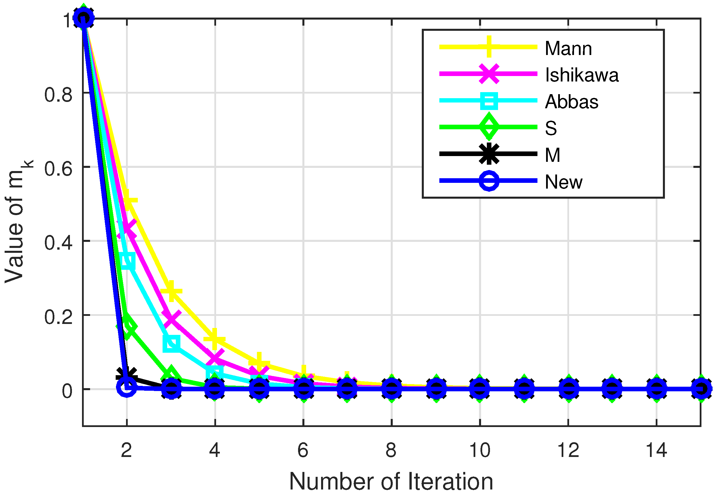
We have also provided some examples of multivalued, almost contractive mappings. We show with the aid of the examples that our iterative algorithm (6) converges faster than many existing iterative algorithms.
(iii)
We have introduced the concepts of weak w 2 -stability and data dependence results involving two multivalued almost contractive mappings. These concepts are relatively new in the literature.
(iv)
We have proved several strong and ∆-convergence results of (6) for the common fixed point of multivalued mappings satisfying condition ( E ) .
(v)
We presented interesting examples of mappings which satisfy condition ( E ) but do not satisfy condition ( C ) . We further performed numerical experiments to compare the efficiency and applicability of our iterative method with some leading iterative algorithms.
(vi)
The results in this article extend and generalize the results in [24,39] and several others from the setting of Banach spaces to the setting hyperbolic spaces. Moreover, our results improve and generalize the results in [22,24,39] and several others from the setting of single-valued mappings to the setting of multivalued mappings. In addition, we improve and extend the results in [22,24,39] from the setting of fixed points of single mapping to the setting common fixed points of two mappings.
(vii)
Our results give affirmative answers to the two interesting open questions raised by Ahmad et al. [21].
(viii)
The main results derived in this article continue to be true in linear and CAT(0) spaces, because the hyperbolic space properly includes these spaces.

Author Contributions

Conceptualization, J.A.A.; Supervision, G.C.U. and O.K.N.; Writing—original draft, A.E.O.; Writing—review & editing, R.G. All authors have read and agreed to the published version of the manuscript.

Funding

This research received no external funding.

Data Availability Statement

The data used to support the findings of this study are included within the article.

Conflicts of Interest

The authors declare that they have no competing interests.

References

  1. Kohlenbach, U. Some logical metatheorems with applications in functional analysis. Trans. Am. Soc. 2005, 357, 89–128. [Google Scholar] [CrossRef] [Green Version]
  2. Goebel, K.; Kirk, W.A. Iteration processes for nonexpansive mappings Topological Methods in Nonlinear Functional Analysis. Contemp. Math. 1983, 21, 115–123. [Google Scholar]
  3. Reich, S.; Shafrir, I. Nonexpansive iterations in hyperbolic spaces. Nonlinear Anal. 1990, 15, 537–558. [Google Scholar] [CrossRef]
  4. Goebel, K.; Reich, S. Uniform Convexity, Hyperbolic Geometry, and Nonexpansive Mappings; Marcel Dekker: New York, NY, USA, 1984. [Google Scholar]
  5. Imdad, M.; Dashputre, S. Fixed point approximation of Picard normal S-iteration process for generalized nonexpansive mappings in hyperbolic spaces. Math. Sci. 2016, 10, 131–138. [Google Scholar] [CrossRef] [Green Version]
  6. Nadler, S.B. Multivalued contraction mappings. Pacific J. Math. 1969, 30, 475–488. [Google Scholar] [CrossRef] [Green Version]
  7. Markin, J. Continuous dependence of fixed point sets. Proc. Am. Math. Soc. 1973, 38, 545–547. [Google Scholar] [CrossRef]
  8. Berinde, V. Approximating fixed points of weak contractions using the Picard iteration. Nonlinear Anal. Forum 2004, 9, 43–53. [Google Scholar]
  9. Berinde, M.; Berinde, V. On a general class of multivalued weakly Picard mappings. J. Math. Anal. 2007, 326, 772–782. [Google Scholar] [CrossRef] [Green Version]
  10. Suzuki, T. Fixed point theorems and convergence theorems for some generalized nonexpansive mappings. J. Math. Anal. Appl. 2008, 340, 1088–1095. [Google Scholar] [CrossRef] [Green Version]
  11. Eslamian, M.; Abkar, A. One-step iterative process for finite family of multivalued mappings. Math. Comput. Model. 2011, 54, 105–111. [Google Scholar] [CrossRef]
  12. García-Falset, J.; Llorens-Fuster, E.; Suzuki, T. Fixed point theory for a class of generalized nonexpansive mappings. J. Math. Anal. Appl. 2011, 375, 185–195. [Google Scholar] [CrossRef] [Green Version]
  13. Kim, J.K.; Pathak, R.P.; Dashputre, S.; Diwan, S.D.; Gupta, R. Convergence theorems for generalized nonexpansive multivalued mappings in hyperbolic spaces. SpringerPlus 2016, 5, 912. [Google Scholar] [CrossRef] [PubMed]
  14. Abdeljawad, T.; Ullah, K.; Ahmad, J.; Mlaiki, N. Iterative approximation of endpoints for Multivalued Mappings in Banach spaces. J. Funct. Spaces 2020, 2020, 2179059. [Google Scholar] [CrossRef]
  15. Chang, S.; Wanga, G.; Wanga, L.; Tang, Y.K.; Mab, Z.L. ∆-convergence theorems for multivalued nonexpansive. Appl. Math. Comput. 2014, 249, 535–540. [Google Scholar]
  16. Karahan, I.; Jolaoso, L.O. A three steps iterative process for approximating the fixed points of multivalued generalized α–nonexpansive mappings in uniformly convex hyperbolic spaces. Sigma J. Eng. Nat. Sci. 2020, 38, 1031–1050. [Google Scholar]
  17. Okeke, G.A.; Abbas, M.; de la Sen, M. Approximation of the mixed Point of multivalued quasi-nonexpansive mappings via a faster iterative process with applications. Discret. Dyn. Nat. Soc. 2020, 2020, 8634050. [Google Scholar] [CrossRef]
  18. Shrama, N.; Mishra, L.N.; Mishra, V.N.; Almusawa, H. Endpoint Approximation of Standard Three-Step Multi-Valued Iteration Algorithm for Nonexpansive Mappings. Appl. Math. Inf. Sci. 2021, 15, 73–81. [Google Scholar]
  19. Agarwal, R.P.; O’Regan, D.; Sahu, D.R. Iterative construction of fixed points of nearly asymptotically nonexpansive mappings. J. Nonlinear Convex Anal. 2007, 8, 61–79. [Google Scholar]
  20. Chuadchawnay, P.; Farajzadehz, A.; Kaewcharoeny, A. On convergence theorems for two generalized nonexpansive multivalued mappings in hyperbolic spaces. Thai J. Math. 2019, 17, 445–461. [Google Scholar]
  21. Ahmad, J.; Ullah, K.; Arshad, M. Convergence, weak w2 stability, and data dependence results for the F iterative scheme in hyperbolic spaces. Numer. Algorithms 2022. [Google Scholar] [CrossRef]
  22. Ali, J.; Jubair, M.; Ali, F. Stability and convergence of F iterative scheme with an application to the fractional differential equation. Eng. Comput. 2020, 38, 693–702. [Google Scholar] [CrossRef]
  23. Khan, A.R.; Fukhar-ud-din, H.; Khan, M.A.A. An implicit algorithm for two finite families of nonexpansive maps in hyperbolic spaces. Fixed Point Theory Appl. 2012, 2012, 54. [Google Scholar] [CrossRef] [Green Version]
  24. Ofem, A.E.; Udofia, U.E.; Igbokwe, D.I. New iterative algorithm for solving constrained convex minimization problem and Split Feasibility Problem. Eur. J. Math. Anal. 2021, 1, 106–132. [Google Scholar] [CrossRef]
  25. Leuştean, L. A quadratic rate of asymptotic regularity for CAT(0) space. J. Math. Anal. Appl. 2007, 325, 386–399. [Google Scholar] [CrossRef] [Green Version]
  26. Soltuz, S.M.; Grosan, T. Data dependence for Ishikawa iteration when dealing with contractive like operators. Fixed Point Theory Appl. 2008, 2008, 242916. [Google Scholar] [CrossRef] [Green Version]
  27. Cardinali, T.; Rubbioni, P. A generalization of the Caristi fixed point theorem in metric spaces. Fixed Point Theory 2010, 11, 3–10. [Google Scholar]
  28. Timis, I. On the weak stability of Picard iteration for some contractive type mappings, Annals of the University of Craiova. Math. Comput. Sci. Ser. 2010, 37, 106–114. [Google Scholar]
  29. Mann, W.R. Mean value methods in iteration. Proc. Am. Math. Soc. 1953, 4, 506–510. [Google Scholar] [CrossRef]
  30. Ishikawa, S. Fixed points and iteration of a nonexpansive mapping in a Banach space. Proc. Am. Math. Soc. 1976, 59, 65–71. [Google Scholar] [CrossRef]
  31. Abbas, M.; Nazir, T. A new faster iteration process applied to constrained minimization and feasibility problems. Mat. Vesnik 2014, 66, 223–234. [Google Scholar]
  32. Ullah, K.; Arshad, M. Numerical Reckoning Fixed Points for Suzuki’s Generalized Nonexpansive Mappings via New Iteration Process. Filomat 2018, 32, 187–196. [Google Scholar] [CrossRef] [Green Version]
  33. Noor, M.A. New approximation schemes for general variational inequalities. J. Math. Anal. Appl. 2000, 251, 217–229. [Google Scholar] [CrossRef] [Green Version]
  34. Phuengrattana, W.; Suantai, S. On the rate off convergence of Mann, Ishikawa, Noor and SP iterations for continuous functions on an arbitrary interval. J. Comput. Appl. Math. 2011, 235, 3006–3014. [Google Scholar] [CrossRef] [Green Version]
  35. Khan, H.S. A Picard-Man hybrid iterative process. Fixed Point Theory Appl. 2013, 2013, 69. [Google Scholar] [CrossRef]
  36. Güsoy, F. A Picard-S iterative Scheme for Approximating Fixed Point of Weak-Contraction Mappings. Filomat 2014, 30, 2829–2845. [Google Scholar] [CrossRef] [Green Version]
  37. Thakurr, B.S.; Thakur, D.; Postolache, M. A new iterative scheme for numerical reckoning of fixed points of Suzuki’s generalized nonexpansive mappings. Appl. Math. Comput. 2016, 275, 147–155. [Google Scholar] [CrossRef]
  38. Chugh, R.; Kumar, V.; Kumar, S. Strong convergence of a new three step iterative scheme in Banach spaces. Am. J. Comput. Math. 2012, 2, 345–357. [Google Scholar] [CrossRef] [Green Version]
  39. Ofem, A.E.; Udofia, U.E.; Igbokwe, D.I. A robust iterative approach for solving nonlinear Volterra Delay integro-differential equations. Ural. Math. J. 2021, 7, 59–85. [Google Scholar] [CrossRef]
Figure 1. Graph corresponding to Table 1.
Mathematics 10 03720 g001
Figure 2. Graph corresponding to Table 2.
Mathematics 10 03720 g002
Figure 3. Graph corresponding to Table 3.
Mathematics 10 03720 g003
Figure 4. Graph corresponding to Table 4.
Mathematics 10 03720 g004
Table 1. Convergence behavior of various iterative algorithms.
m k MannIshikawaAbbasSMNew
m 1 1.0000001.0000001.0000001.0000001.0000001.000000
m 2 0.5125000.4332810.3480680.1707810.0320310.003557
m 3 0.2626560.1877330.1211520.0291660.0010260.000000
m 4 0.1346110.0813410.0421690.0049810.0000330.000000
m 5 0.0689880.0352440.0146780.0008510.0000010.000000
m 6 0.0353570.0152700.0051090.0001450.0000000.000000
m 7 0.0181200.0066160.0017780.0000250.0000000.000000
m 8 0.0092870.0028670.0006190.0000040.0000000.000000
m 9 0.0047590.0012420.0002150.0000010.0000000.000000
m 10 0.0024390.0005380.0000750.0000000.0000000.000000
m 11 0.0012500.0002330.0000260.0000000.0000000.000000
m 12 0.0006410.0001010.0000090.0000000.0000000.000000
m 13 0.0003280.0000440.0000030.0000000.0000000.000000
m 14 0.0001680.0000190.0000010.0000000.0000000.000000
m 15 0.0000860.0000080.0000000.0000000.0000000.000000
The reds show the point of convergence of various iterative methods.
Table 2. Convergence behavior of various iterative algorithms.
m k NoorSPPicard-ManPicard-SFNew
m 1 1.0000001.0000001.0000001.0000001.0000001.000000
m 2 0.4583200.1346110.1281250.0426950.0080080.003557
m 3 0.2100580.0181200.0164160.0018230.0000640.000000
m 4 0.0962740.0024390.0021030.0000780.0000010.000000
m 5 0.0441240.0003280.0002690.0000030.0000000.000000
m 6 0.0202230.0000440.0000350.0000000.0000000.000000
m 7 0.0092690.0000060.0000040.0000000.0000000.000000
m 8 0.0042480.0000010.0000010.0000000.0000000.000000
m 9 0.0019470.0000000.0000000.0000000.0000000.000000
The reds show the point of convergence of various iterative methods.
Table 3. Convergence behavior of various iterative algorithms.
m k MannIshikawaSPicard-MannFNew
m 1 5.000000005.000000005.000000005.000000005.000000005.00000000
m 2 4.375000004.140625003.515625003.281250001.845703130.99609375
m 3 3.828125003.428955082.471923832.153320310.681324010.19844055
m 4 3.349609382.839603421.738071441.413116460.251504370.03953308
m 5 2.930908202.351546591.222081480.927357670.092840480.00787573
m 6 2.564544681.947374520.859276040.608578470.034271190.00156899
m 7 2.243976591.612669520.604178470.399379620.012650890.00031257
m 8 1.963479521.335491950.424812980.262092880.004669960.00006227
m 9 1.718044581.105954270.298696630.171998450.001723870.00001241
m 10 1.503289010.915868380.210021070.112873980.000636350.00000247
m 11 1.315377880.758453500.147671060.074073550.000234900.00000049
m 12 1.150955650.628094310.103831220.048610770.000086710.00000010
m 13 1.007086190.520140600.073006320.031900820.000032010.00000002
m 14 0.881200420.430741430.051332570.020934910.000011820.00000000
The reds show the point of convergence of various iterative methods.
Table 4. Convergence behavior of various iterative algorithms.
m k NoorCRThakurPicard-SMNew
m 1 5.000000005.000000005.000000005.000000005.000000005.00000000
m 2 4.052734382.119140632.636718751.816406252.460937500.99609375
m 3 3.284931180.898151401.390457150.659866331.211242680.19844055
m 4 2.662590700.380661820.733248890.239717070.596158500.03953308
m 5 2.158154580.161335190.386674220.087084720.293421760.00787573
m 6 1.749285450.068378390.203910230.031636240.144418520.00156899
m 7 1.417877850.028980680.107530790.011492850.071080990.00031257
m 8 1.149256460.012282830.056705690.004175140.034985180.00006227
m 9 0.931526230.005205810.029903390.001516750.017219270.00001241
m 10 0.755045680.002206370.015769370.000551010.008475110.00000247
m 11 0.611999910.000935120.008315880.000200170.004171340.00000049
m 12 0.496054620.000396330.004385330.000072720.002053080.00000010
m 13 0.402075520.000167980.002312570.000026420.001010500.00000002
m 14 0.325901060.000071190.001219520.000009600.000497360.00000000
The reds show the point of convergence of various iterative methods.
Publisher’s Note: MDPI stays neutral with regard to jurisdictional claims in published maps and institutional affiliations.

