Abstract
Land cover classification is critical for urban sustainability applications. Although deep convolutional neural networks (DCNNs) have been widely utilized, they have rarely been used for land cover classification of complex landscapes. This study proposed the prior knowledge-based pretrained DCNNs (i.e., VGG and Xception) for fine land cover classifications of complex surface mining landscapes. ZiYuan-3 data collected over an area of Wuhan City, China, in 2012 and 2020 were used. The ZiYuan-3 imagery consisted of multispectral imagery with four bands and digital terrain model data. Based on prior knowledge, the inputs of true and false color images were initially used. Then, a combination of the first and second principal components of the four bands and the digital terrain model data (PD) was examined. In addition, the combination of red and near-infrared bands and digital terrain model data (43D) was evaluated (i.e., VGG-43D and Xcep-43D). The results indicate that: (1) the input of 43D performed better than the others; (2) VGG-43D achieved the best overall accuracy values; (3) although the use of PD did not produce the best models, it also provides a strategy for integrating DCNNs and multi-band and multimodal data. These findings are valuable for future applications of DCNNs to determine fine land cover classifications in complex landscapes.
1. Introduction
Land cover classification [1,2,3,4] is widely studied in the remote sensing community, and its corresponding products (e.g., roads in complex environments [5,6] and semantic level results of scene classification [7,8] etc.) are very useful for various earth science and urban sustainability applications [2,9]. Presently, determining land cover classification in complex landscapes, particularly fine land cover classification, has many challenges [10,11,12]. Thus, corresponding algorithm and application research are of great significance. Although determining the land cover classification and fine land cover classification of complex surface mining landscapes has been conducted in previous studies [13,14,15,16,17,18,19,20], it deserves further investigation.
With recent developments in optical imagery, high spatial resolution topographic data and object-oriented analysis technology [21], determining land cover classification and fine land cover classification in complex landscapes, have achieved some advances [22]. However, the low-level spectral–spatial and topographic features based on feature engineering [17,22,23,24,25] are far from sufficient for characterizing the complex patterns present within complex landscapes.
Deep learning is a type of end-to-end feature extraction and classification algorithm that has been applied with great success in computer vision and remote sensing research [26,27]. The main deep learning methods include the restricted Boltzmann machine-based deep belief network (DBN) [28], stacked autoencoder [29,30,31], and convolutional neural networks (CNNs) [32]. CNNs are the most utilized deep learning algorithm in remote sensing applications [33,34,35,36]. For fine land cover classification of complex surface mining landscapes, Li et al. [18] combined DBN and two machine learning classifiers (i.e., random forest and support vector machine). They [19] also examined multi-level output-based DBN and CNN algorithms. Qian et al. [20] used a multimodal data and multiscale kernel-based multistream CNN model. However, complex deep learning algorithms often require a large amount of sample data. Remote sensing image classification is a natural case of few samples, especially for fine land cover classification. In the case of few samples, it is challenging to determine how to provide more input information and guide the design of deep learning models based on prior knowledge, in order to obtain effective feature representations.
Designs of shallow CNN models are effective. For example, Li et al. [37], Xu et al. [38], Chen et al. [39,40], Jahan et al. [41], and Rasti et al. [42] applied multistream CNN models based on hyperspectral image and light detection and ranging data. Zhang et al. [43,44] utilized multiscale feature-based CNN models. For fine land cover classification of complex surface mining landscapes, Qian et al. [20] used a three-stream CNN model. However, the structures and hyper-parameters of those models were application-specific and data-specific, with poor generalization ability.
Recently, the emergence of deep CNNs (DCNNs), such as VGG [45] and Xception [46], has advanced the remote sensing scene classification process [47,48]. One of the most important advances can be attributed to the ImageNet-based [49] pretrained network, which can be used to directly extract features or for further fine-tuning with limited amounts of labeled data [50]. DCNNs have been applied to land cover classification in some complex landscapes. For example, Mahdianpari et al. [50] successfully used several DCNNs to map complex wetlands. Rezaee et al. [51] utilized AlexNet to classify complex wetland. Dang et al. [52] conducted coastal wetland classification with a deep U-Net model. Zhao et al. [53] performed a preliminary classification of cropland, forest, buildup, and water in a complex landscape by the pretrained CNN method. Moreover, Mahdianpari et al. [50] and Rezaee et al. [51] used a correlation analysis for multispectral imagery to pick out three bands as the input of DCNN models. Thus, whether the DCNN is suitable for fine land cover classification in complex surface mining landscapes is uncertain and requires further investigation. In particular, how to integrate the spectral bands and topographic information into a DCNN with three informative input bands is an issue.
This study aimed to (1) investigate the performance of the prior knowledge-based DCNN models for determining fine land cover classification in complex surface mining landscapes, (2) compare different combinations of spectral bands as the inputs for different DCNNs to determine fine land cover classification in complex surface mining landscapes, and (3) propose a pipeline process for applying multi-band and multi-source remote sensing data in DCNN-based classifications.
2. Materials and Methods
2.1. Study Area and Satellite Remote Sensing Data
The study area was located in Wuhan City, China, with an area of 109.4 km2 [15,17] (Figure 1). The study area included seven main land cover types: water, road, forest land, crop land, residential land, bare land, and surface mining land [17]. Moreover, the land cover types were characterized as complex surface mining landscapes by previous studies [17]. This was an ideal study area because it contains high intraclass differences and interclass similarities [50], significant positive and negative terrain [54,55], and large spatiotemporal variation changes [56,57]. In this study, we mainly focused on determining the fine classification of the land cover subclasses [17].
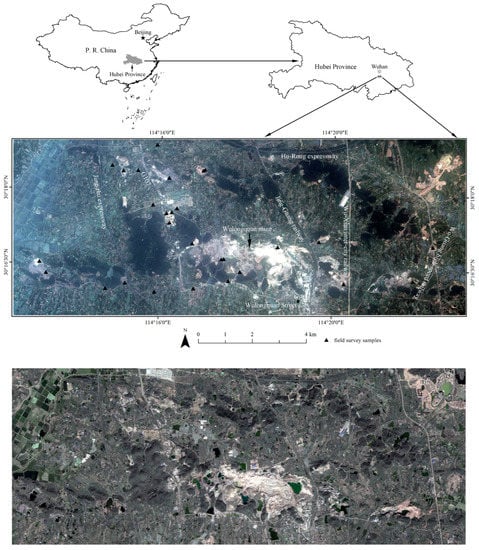
Figure 1.
ZiYuan-3 true-color imagery (using red, green, and blue bands for color composition) on 20 June 2012 [17] (top) and 11 November 2020 [20] (bottom), and location of the study site and field sampling points [17].
Satellite imagery acquired on 20 June 2012 by ZiYuan-3 was utilized in this study [17]. First, the stereo image pairs, i.e., the front and backward-facing images (3.6 m), were used to extract the digital terrain model data with a spatial resolution of 10 m. Then, panchromatic and multispectral images (2.1 m and 5.8 m, respectively) were used to construct a 2.1 m multispectral image based on the Gram–Schmidt fusion method. Finally, digital terrain model was resampled to 2.1 m.
Another ZiYuan-3 image from 11 November, 2020 was also used in this study (Figure 1) [20]. The fused multispectral image and digital terrain model data were also obtained. These two data could help to evaluate the model performance.
2.2. Prior Knowledge-Based DCNN Models
Figure 2 shows the flowchart of the prior knowledge-based DCNN model. First, some spectral-spatial and topographic features were extracted from the multimodal multispectral imagery and digital terrain model data. Then, based on prior knowledge, some selections of three features for combinations were used as input data. Subsequently, input patches were extracted and resized. The resulted input patches were then used for fine-tuning of the pretrained DCNN models. Finally, the models were assessed and analyzed.
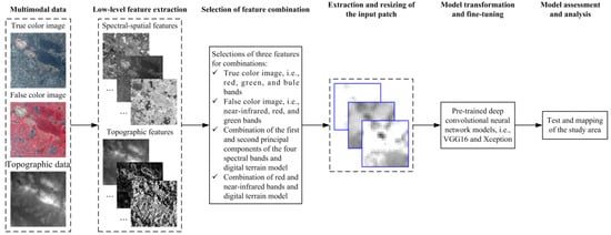
Figure 2.
Flowchart of prior knowledge-based deep convolutional neural network model (the subset images were from the data in 2012).
2.2.1. Prior Knowledge-Based Inputs
To directly transfer the pretrained DCNN models, the input data only needed three bands. Naturally, two band combinations (true and false color images) can be used as inputs (i.e., DCNN-321 and DCNN-432). Especially, Qian et al. [20] proved that true and false color images had different feature representation capabilities and were effective for fine land cover classification of complex surface mining landscapes.
Considering that four spectral bands and topographic data from the digital terrain model were available, two principal components for the multispectral imagery and digital terrain model data (PD) (DCNN-PD) were combined. Moreover, Li et al. [17] indicated that the two principal components could represent the multispectral image, with a cumulative contribution rate of 98.99%. Figure 3 shows the images of these two components. It can be seen that there were some visual differences for the land covers of water, road, vegetation, and mining areas, etc.
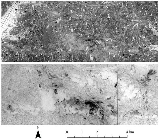
Figure 3.
Images of the first two principal components.
Moreover, a combination of the red and near-infrared bands and digital terrain model data (43D) (DCNN-43D) was used as inputs. The prior knowledge of using red and near-infrared bands could be obtained from the feature selection results in Li et al. [17], which indicated that for spectral bands only the red and near-infrared bands with higher importance were selected.
Furthermore, Li et al. [17] and Chen et al. [15] revealed that the digital terrain model was one of the most important features for fine land cover classification of complex surface mining landscapes.
For each pixel, the neighborhood patch was used as the input for the DCNNs [58]. The scale of the input patch was identified based on a trial-and-error method [59], from which a 15 × 15 pixel scale was selected [20]. Qian et al. [20] indicated that the pixel neighbor scale of 15 × 15 can depict the features of pixel’s land cover classes and the surroundings (for details, see Figures 5 and 6 in [20]). The patch size of 15 × 15 pixels was then resized to 128 × 128 pixels for the DCNNs by using bilinear interpolation method.
2.2.2. Transformation and Fine-Tuning of DCNNs
The pretrained VGG16 and Xception (for details see Section 2.2.3) models and a fine-tuning strategy were used in this study. The number of epochs and the batch size were 200 and 256, respectively. Adam was selected as the optimization algorithm. The learning rate was 0.0001. All of the models were programmed based on the Python software and the TensorFlow framework. The machine used for the computations had two Intel Xeon E5-2603 v4 CPUs, 128 GB of memory, and two NVIDIA GeForce GTX 1080 Ti GPUs.
Then, the models of VGG-321, Xcep-321, VGG-432, Xcep-432, VGG-PD, Xcep-PD, VGG-43D, and Xcep-43D were constructed.
By using training and validation sets, the optimal epochs were selected when the accuracies of the validation set reached the highest values. The accuracy and loss curves for training and validation sets and the optimal epoch values are shown in Figures S1–S8. When the epoch reached 50, the accuracies and losses of the validation set were stable.
2.2.3. VGG and Xception Networks
The VGG algorithm [45] is a typical DCNN that contains some small convolution operations, with kernels of 3 pixels × 3 pixels (Figure 4). VGG16 includes 13 convolution and three fully connected layers. Moreover, there are five max-pooling layers with no parameters and one Softmax layer used for classification [47].
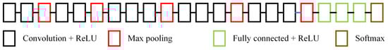
Figure 4.
Schematic diagram of the VGG16 network [45].
The Xception network [46] is a revised version of inception (GoogLeNet), in which the inception module is replaced by depth-wise separable convolutions (Figure 5). Moreover, the Xception algorithm is stacked with several normal depth-wise separable 1 × 1 convolutional layers [60].
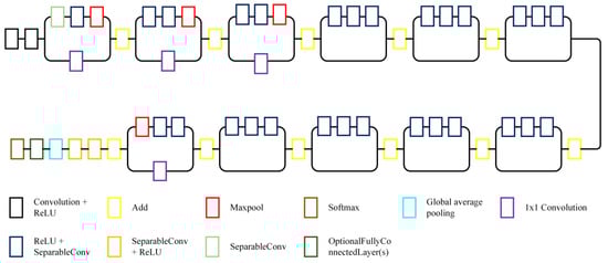
Figure 5.
Schematic diagram of the Xception network [46].
2.3. Training, Validation, and Test Data
Five sets of training, validation, and test data were derived from a group of data polygons in the study area by using the stratified random sampling strategy. The numbers of data polygons and data fractions are shown in Table 1. For each land cover subclass, these three datasets included 2000, 500, and 500 sample points (Table 1). The data polygons utilized in this study were obtained from Li et al. [18]. The training, validation, and test data were randomly selected and were independent (for details, see Figure 5 in [18]). Only the total pixels of six subclasses exceeded 20% of the number of pixels in the corresponding data polygons. The training, validation, and test data were used for model development and accuracy assessment [61].

Table 1.
Number and area (km2) of the data polygons (DPs) and the fractions (%) of the number of pixels in the training, validation, and test data [18]. Fraction 1: the ratio of the numbers of pixels in the training data and the DPs. Fraction 2: the ratio of the numbers of pixels in the validation (test) data and the DPs. Fraction 3: the ratio of the numbers of pixels in the three datasets and the DPs.
Similarly, the training, validation, and test sets of the imagery in 2020 were also with 2000, 500, and 500 random samples for each subclass, respectively [20].
2.4. Accuracy Evaluation Metrics
Three metrics (i.e., overall accuracy, F1-score, and Kappa coefficient) were used to quantify the total performances of all of the models. The F1-measure [62] was calculated to assess the accuracy of each land cover subclass. Five repeated runs were conducted for each experiment, and the mean and standard deviation values were calculated for those four metrics. The percentage deviation value [63] that conducted on the mean values of those four metrics was applied to evaluate performance differences among the different models.
3. Results and Discussion
3.1. Overall Performance Assessment
3.1.1. Assessment for Imagery in 2012
The overall performances of the proposed and former models are listed in Table 2. The corresponding percentage deviation values are listed in Tables S1–S3. In all of the models, the overall accuracy values decreased in the order of VGG-43D, Xcep-43D, Xcep-321, VGG-321, Xcep-432, Xcep-PD, VGG-PD, and VGG-432. This order was the same for Kappa and the F1-score. The best-performing model was obviously VGG-43D. Moreover, the 43D input overtook the others. Li et al. [17] performed a feature selection for land cover classifications of complex surface mining landscapes and found that: (1) the digital terrain model had the highest importance, and (2) for four spectral bands, only the red and near-infrared bands were picked out. This may explain the superiority of using 43D as the input data. Based on the different inputs, almost all of the Xception models outperformed the VGG models, with the exception of VGG-43D and Xcep-43D. It also can be seen from Table 2 that VGG-43D outperformed all the traditional machine learning algorithms, DBN, and CNN-based models in [18,19,20], respectively.
Table 2.
Overall performances of the models by using imagery in 2012.
With respect to the true color imagery and PD inputs, the percentage deviations of the overall accuracy, Kappa, and F1-score metrics between Xception and VGG ranged from 3.95% to 7.44% (Table S1). For the false color imagery input, the differences were very large, with corresponding percentage deviations of 15.95%, 17.12%, and 16.06%, respectively. However, the VGG-43D model overtook the Xcep-43D model. Compared to the utilization of other inputs, the accuracy differences of Xcep-432 and VGG-432 were very large. The false color imagery is only discriminative for land covers of water and vegetation, etc. Compared to VGG, the deeper structure of Xception can extract more effective features from the false color imagery. Perhaps this was the reason for the superiority of Xcep-432.
Based on the VGG network, the 43D input yielded the best performance, while the false color imagery input yielded the worst performance (Table S2). Compared to the VGG-based models using true and false color images and PD inputs, the VGG-43D model yielded improvements ranging from 10.55% to 33.50% in its overall accuracy, Kappa, and F1-score metrics. Similarly, compared to the VGG-based models using false color images and PD inputs, the VGG-321 model yielded improvements ranging from 13.40% to 20.07%. In addition, the VGG-PD model outperformed the VGG-432 model, with metric improvements of about 5%.
In the Xception network, the 43D input yielded the best model performance, while the PD input resulted in the worst performance (Table S3). Similarly, compared to the Xception-based models using true and false color images and PD inputs, the Xcep-43D model increased the overall accuracy, Kappa, and F1-score values by 2.40% to 13.88%. Compared to the Xception-based models using false color images and PD inputs, the Xcep-321 model increased by 6.51% to 11.10%. Additionally, the Xcep-432 model performed better than the Xcep-PD model (with improvements of about 4%).
3.1.2. Assessment for Imagery in 2020
Table 3 presents the overall accuracy, Kappa, and F1-score values for imagery on 11 November 2020. The corresponding percentage deviation values are listed in Tables S4–S6. Similarly, the 43D input overtook the others. On the contrary, based on the different inputs, almost all of the VGG models outperformed the Xception models. Due to the time of ZiYuan-3 imagery, some land covers were hard to classify. Perhaps the strategy proposed in this study reached an accuracy bottleneck. As such, the deeper structure of Xception may have negative effect. Moreover, the 432 input outperformed 321. The VGG-PD had a better performance than VGG-321, and Xcep-PD overtook Xcep-432 and Xcep-321. Perhaps due to the time of the ZiYuan-3 imagery, the proposed models were not very good, and obviously worse than the CNN-based models in [20]. It is worth further investigating this in the future.
Table 3.
Overall performances of the models by using imagery in 2020.
With respect to all the inputs, the percentage deviations of the overall accuracy, Kappa, and F1-score metrics between VGG and Xception were not large, ranging from 2.11% to 5.57% (Table S4).
Based on the VGG network, the 43D input yielded the best performances, while the true color imagery input yielded the worst performances (Table S5). Similarly, different input-based models have small differences, ranging from 0.40% to 3.09%.
Table S6 shows the percentage deviations from different input-based Xception models. Similarly, the 43D input yielded the best model performances, and the true color imagery input resulted in the worst performances. Moreover, the differences only ranged from 0.35% to 6.12%.
3.2. Assessment of the Predicted Maps
3.2.1. Assessment of the Maps in 2012
The predicted maps of the study area derived from the VGG-43D (Figure 6b), Xcep-43D (Figure 6c), and Xcep-321 (Figure 6e) models, the DBN-based support vector machine algorithm in Li et al. [18] (Figure 6d), and that from the multimodal data and multiscale kernel-based multistream convolutional neural network with the selected value of parameter k [20] (Figure 6a) are shown in Figure 6. The VGG-43D model achieved both better test accuracy values and visual accuracy. However, the DBN-based support vector machine algorithm yielded higher overall accuracy values (i.e., 94.74% ± 0.35%) (Li et al. [18]) than the Xcep-43D and Xcep-321 models, and its visual accuracy of the study area was obviously worse. The bare land, residential land, dumping ground, roads, ore-processing sites, and pond and stream areas (i.e., areas 1–6 in Figure 6) in this study were all classified more accurately. Moreover, compared to VGG-43D model, the multimodal data and multiscale kernel-based multistream convolutional neural network with the selected value of parameter k [20] achieved better performances on woodland and ore-processing sites, and worse results on bare surface.
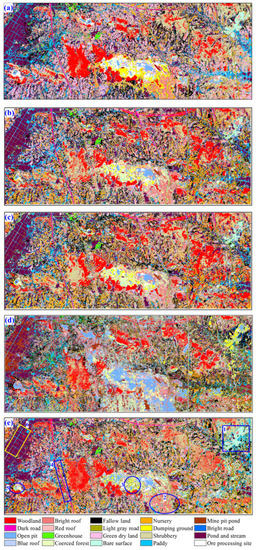
Figure 6.
Predicted maps of the study area derived from the VGG-43D (b), Xcep-43D (c), and Xcep-321 (e) models, the deep belief network-based support vector machine model in Li et al. [18] (d), and that from the multimodal data and multiscale kernel-based multistream convolutional neural network with the selected value of parameter k [20] (a) by using imagery in 2012. Numbers 1–6 represent the areas with different predicted classes that derived from those above-mentioned models.
The predicted map of the study area derived from the VGG-PD and VGG-432 models are shown in Figure 7. The VGG-PD model outperformed the VGG-432 model, particularly in areas 1 and 3 in Figure 7, as some woodlands were misclassified by the VGG-432 model. For areas 2, 4, and 5, some of the open pit classes were also incorrectly classified by the VGG-432 model.
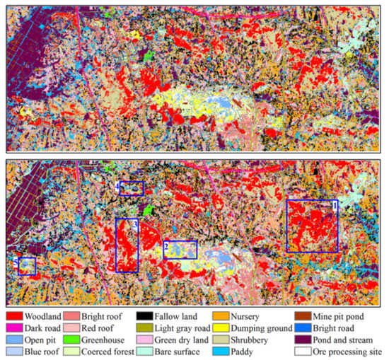
Figure 7.
Predicted maps of the study area derived from the VGG-PD (bottom) and VGG-432 (top) models by using imagery in 2012. Numbers 1–5 represent the areas with different predicted classes that derived from those above-mentioned models.
3.2.2. Assessment of the Maps in 2020
The predicted map of the study area derived from the VGG-432 (Figure 8b), VGG-PD (Figure 8c), and VGG-43D (Figure 8d) models, and that from the multimodal data and multiscale kernel-based multistream convolutional neural network with the selected value of parameter k [20] (Figure 8a)—by using ZiYuan-3 imagery on 11 November 2020—are shown in Figure 8. For the rectangular areas, there were some visual differences among the predicted maps. The multimodal data and multiscale kernel-based multistream convolutional neural network with the selected value of parameter k [20] achieved obviously better performances on paddy field, bright roof, bare surface land, harvest land, and mining lands, etc. For area 1, some water was wrongly classified by multiscale kernel-based multistream convolutional neural network with the selected value of parameter k [20] and VGG-PD. For area 2, some dumping ground lands were misclassified by VGG-PD and VGG-43D. For area 3, some open pit and dumping ground lands were misclassified by the VGG-432, VGG-PD, and VGG-43D model. For area 4, some dumping ground lands were also wrongly classified bye the three models of VGG-432, VGG-PD, and VGG-43D.
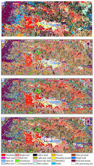
Figure 8.
Predicted maps of the study area derived from the VGG-432 (b), VGG-PD (c), and VGG-43D (d) models, and that from the multimodal data and multiscale kernel-based multistream convolutional neural network with the selected value of parameter k [20] (a) by using imagery in 2020. Numbers 1–4 represent the areas with different predicted classes that derived from those above-mentioned models.
3.3. Assessment of Different Land Cover Accuracies
3.3.1. Assessment of Each Land Cover for Imagery in 2012
The assessment of different land cover accuracies was conducted on imagery from 2012. The F1-measures of the land cover subclasses based on each of the models are listed in Table 4. The corresponding percentage deviation values are listed in Tables S7–S9. The performances of all models (Table 4) based on the subclass F1-measures exhibited the same decreasing order as that described in Section 3.1.1, with some exceptions. For example, based on the different inputs, the Xception-based models achieved larger F1-measures for almost all of the land cover types than the VGG-based models, with only four exceptions (i.e., percentage deviation values less than 0 in Table S7). Based on the VGG network, the 43D input resulted in the best performance for over half of the land cover types, while the false color imagery input yielded the worst performance (exceptions are negative values in Table S8). Based on the Xception network, the 43D input yielded the best performance for over half of the land cover types, while the PD input yielded the worst (exceptions are negative values in Table S9).
Table 4.
F1-measures (%) for each land cover subclass based on all models by using imagery in 2012 (Numbers 1–20 represent the subclasses in Table 1).
Compared to the others, it was perhaps the less spectral information and topographic data with low resolution in 43D that resulted in the poor performance of class 6 (shrubbery), similarly to PD. Between class 13 (dirt road) and the surroundings, there were both spectral and topographic differences. As a result, the inputs of 43D and PD yielded better results; the 43D-based models in particular obtained obvious improvements.
For the best model (VGG-43D), 90% of the land cover types achieved F1-measures over 90% (Table 4). Only two land cover types (trees and shrubbery) had over 80% accuracy values. However, for the worst model (VGG-432), 60% of the land cover subclasses achieved less than 80% accuracy (Table 4), i.e., coerced forests, nurseries, ponds, asphalt roads, dirt roads, buildings with bright roofs, buildings with red roofs, buildings with blue roofs, bare land, surface mining, mine selection sites, and dumping land.
With respect to the true color imagery, all F1-measures for the land cover types derived from the Xception network were always larger than those derived from the VGG network. The corresponding percentage deviation values ranged from 0.07% to 9.76%, with an average value of 4.10%. Only 40% of the subclasses achieved over 5% improvements, i.e., harvested land, coerced forests, nurseries, asphalt roads, buildings with blue roofs, surface mining, mine selection sites, and dumping land. For the false color imagery, the F1-measures of two subclasses derived from the Xception network were smaller than those derived from the VGG network, i.e., harvested land and trees, with percentage deviations of −0.16% and −3.86%, respectively. The other subclasses had larger F1-measures (ranging from 2.27% to 57.34%, with an average of 21.08%). In addition, 50% of the subclasses achieved over 20% improvement. Similarly, for the PD input, the F1-measure values of two subclasses derived from the Xception network were smaller than those derived from the VGG network, i.e., harvested land and trees, with percentage deviations of −0.23% and −1.61%, respectively. Conversely, the other subclasses had larger F1-measures (ranging from 0.64% to 30.66%, with an average of 10.16%). Additionally, 30% of the subclasses achieved over 10% improvement in their scores. For the 43D input, all F1-measures for the land cover types derived from the VGG network were greater than those derived from the Xception network. The corresponding percentage deviations ranged from 0.08% to 11.19%, with an average of 4.02%, and only 40% of the subclasses achieved greater than 5% improvement in their F1-measures.
For the VGG network, almost all F1-measures of the land cover types based on the 43D input were larger than those of the other inputs, with the exception of trees and shrubbery. In particular, some very large percentage deviations were observed for dirt roads and coerced forests. For the VGG network, all of the land cover types’ F1-measures based on true color imagery were greater than those based on false color imagery. The corresponding percentage deviations ranged from 0.01% to 69.45%, with an average of 22.33%. In addition, 50% of the subclasses achieved over 20% improvement in their F1-measures. Five subclasses’ F1-measure values based on true color imagery were smaller than those based on the PD input (ranging from −9.24% to −0.08%, with an average of −3.67%), while the opposite was true for the other subclasses (ranging from 3.76% to 65.88%, with an average of 24.76%). Five subclasses achieved over 20% improvement in their scores. Similarly, seven subclasses’ F1-measure values based on the PD input were smaller than those based on false color imagery (ranging from −25.36% to −2.58%, with an average of −15.49%), while the opposite was true for the other subclasses (ranging from 1.26% to 58.57%, with an average of 19.21%). Nine subclasses achieved over 20% improvement or decreases in their scores.
For the Xception network, 40% of the land covers’ F1-measures based on the 43D input were smaller than those based on true color imagery. However, for the other land cover types, almost all the F1-measures based on the 43D input were larger. Some large percentage deviations were observed for dirt roads and coerced forests. Almost all of the land covers’ F1-measures based on true color imagery were greater than those based on false color imagery, with only one exception, i.e., greenhouse sheds. For the other subclasses, the corresponding percentage deviations ranged from 0.42% to 17.48%, with an average of 7.40%. Only five subclasses achieved over 10% improvement in their F1-measures. Three subclasses’ F1-measure values based on true color imagery were smaller than those based on the PD input (ranging from −9.88% to −0.75%, with an average of −5.31%), while the opposite was true for the other subclasses (ranging from 0.83% to 40.62%, with an average of 14.62%). Five subclasses achieved over 20% improvement in their F1-measures. Similarly, eight subclasses’ F1-measure values based on false color imagery were smaller than those based on the PD input (ranging from −17.24% to −0.32%, with an average of −6.97%), while the opposite was true for the other subclasses (ranging from 0.50% to 26.65%, with an average of 11.92%). Only three subclasses achieved over 20% improvement in their F1-measures.
3.3.2. Assessment of Each Land Cover for Imagery in 2020
The assessment of different land cover accuracy values was conducted on imagery from 2020. The F1-measures of the land cover subclasses based on each of the models are listed in Table 5. The corresponding percentage deviation values are listed in Tables S10–S12. The performances of all models (Table 5), based on the subclass F1-measures, exhibited the same decreasing order as that described in Section 3.1.2, with some exceptions. For example, based on the different inputs, the VGG-based models achieved larger F1-measures for almost all of the land cover types than the Xception-based models, with twenty one exceptions (i.e., percentage deviation values less than 0 in Table S10). Based on the VGG network, the 43D input resulted in the best performance for over half of the land cover types, while the true color imagery input yielded the worst performance (exceptions are negative values in Table S11). Based on the Xception network, the 43D input yielded the best performance for over half of the land cover types, while the true color imagery input yielded the worst (exceptions are negative values in Table S12).
Table 5.
F1-measures (%) for each land cover subclass based on all models by using imagery in 2020 (Numbers 1–20 represent the subclasses in Table 1).
For the best model (VGG-43D), 65% of the land cover types achieved F1-measures over 90% (Table 5). Only four land cover types (i.e., farming dry land, nursery, building with bright roof, and bare land) had over 80% accuracy values. However, for the worst model (Xcep-321), 35% of the land cover subclasses achieved less than 80% accuracy (Table 5).
With respect to the true color imagery, almost all F1-measures for the land cover types derived from the VGG network were always larger than those derived from the Xception network (with only three exceptions). For the false color imagery, the F1-measures of three subclasses derived from the Xception network were larger than those derived from the VGG network. For the PD input, the F1-measure values of thirteen subclasses derived from the Xception network were larger than those derived from the VGG network. For the 43D input, almost all F1-measures for the land cover types derived from the VGG network were greater than those derived from the Xception network (with only three exceptions).
For the VGG network, almost all F1-measures of the land cover types based on the 43D input were larger than those of the true color imagery inputs, with the exception of water in the mine pit, building with bright roof, and mine selection site.
For the VGG network, almost all of the land cover types’ F1-measures based on false color imagery were greater than those based on true color imagery (with only two exceptions). Seven subclasses’ F1-measure values based on false color imagery were smaller than those based on the PD input. Similarly, four subclasses’ F1-measure values based on the PD input were smaller than those based on true color imagery.
For the Xception network, only four land covers’ F1-measures based on the 43D input were smaller than those based on true color imagery. However, eight and sixteen land covers’ F1-measures based on false color imagery and PD were larger than those based on 43D. Almost all of the land covers’ F1-measures based on true color imagery were greater than those based on false color imagery, with only one exception. Four subclasses’ F1-measure values based on true and false color images were larger than those based on the PD input.
4. Conclusions
In this study, the prior knowledge-based pretrained VGG and Xception models were used to investigate the fine land cover classification of complex surface mining landscapes using ZiYuan-3 imagery from 2012 and 2020 in Wuhan City, China. First, the ZiYuan-3 imagery was processed. Then, fused multispectral imagery with four bands and digital terrain model data were obtained. Considering the three channels required for the DCNNs, the following four inputs were proposed and compared: true color imagery, false color imagery, a combination of the first and second principal components of four bands and digital terrain model, and a combined input of the red and near-infrared bands and digital terrain model data. Five sets of training, validation, and test data with 20 subclasses were constructed and used for the model development and accuracy assessments. A neighborhood patch of 15 × 15 pixels was used for each pixel and resized to 128 × 128 as the input for the DCNNs.
The results indicate that: (1) models with the 43D input performed better than those with true and false color images and PD inputs; (2) with different imageries, VGG and Xception-based models achieved different performances; (3) the VGG-43D model achieved the best overall accuracies (96.44% ± 0.20% for imagery in 2012 and 88.15% ± 0.32% for imagery in 2020); (4) although the use of PD did not produce the best models, it also provides a strategy for integrating DCNNs and multi-band and multimodal data. In addition, the predicted maps of the study area were very accurate. Future research should focus on achieving better integrations of multispectral and topographic data into DCNNs for determining land cover classification in complex landscapes.
Supplementary Materials
The following supporting information can be downloaded at: https://www.mdpi.com/article/10.3390/su141912563/s1. Figure S1: the accuracy and loss curves for training and validation sets, and the optimal epoch values based on the model of VGG-321; Figure S2: the accuracy and loss curves for training and validation sets, and the optimal epoch values based on the model of Xcep-321; Figure S3: the accuracy and loss curves for training and validation sets, and the optimal epoch values based on the model of VGG-432; Figure S4: the accuracy and loss curves for training and validation sets, and the optimal epoch values based on the model of Xcep-432; Figure S5: the accuracy and loss curves for training and validation sets, and the optimal epoch values based on the model of VGG-PD; Figure S6: the accuracy and loss curves for training and validation sets, and the optimal epoch values based on the model of Xcep-PD; Figure S7: the accuracy and loss curves for training and validation sets, and he optimal epoch values based on the model of VGG-43D; Figure S8: the accuracy and loss curves for training and validation sets, and the optimal epoch values based on the model of Xcep-43D; Table S1: percentage deviations (%) of the overall accuracy, Kappa, and F1-score metrics based on two different algorithms, with the same inputs from the ZiYuan-3 imagery in 2012; Table S2: percentage deviations (%) of the overall accuracy, Kappa, and F1-score metrics between VGG-based models, with different inputs from the ZiYuan-3 imagery in 2012; Table S3: percentage deviations (%) of the overall accuracy, Kappa, and F1-score metrics between Xception-based models, with different inputs from the ZiYuan-3 imagery in 2012; Table S4: percentage deviations (%) of the overall accuracy, Kappa, and F1-score metrics based on two different algorithms, with the same inputs from the ZiYuan-3 imagery in 2020; Table S5: percentage deviations (%) of the overall accuracy, Kappa, and F1-score metrics between VGG-based models, with different inputs from the ZiYuan-3 imagery in 2020; Table S6: percentage deviations (%) of the overall accuracy, Kappa, and F1-score metrics between Xception-based models, with different inputs from the ZiYuan-3 imagery in 2020; Table S7: percentage deviations (%) of the F1-measure values for each land cover subclass derived from two different models, with the same inputs from the ZiYuan-3 imagery in 2012 (Numbers 1–20 represent the subclasses in Table 1); Table S8: percentage deviations (%) of F1-measure values for each land cover subclass derived from VGG-based models, with different inputs from the ZiYuan-3 imagery in 2012 (Numbers 1–20 represent the subclasses in Table 1); Table S9: percentage deviations (%) of the F1-measure values for each land cover subclass derived from Xception-based models, with different inputs from the ZiYuan-3 imagery in 2012 (Numbers 1–20 represent the subclasses in Table 1); Table S10: percentage deviations (%) of the F1-measure values for each land cover subclass derived from two different models, with the same inputs from the ZiYuan-3 imagery in 2020 (Numbers 1–20 represent the subclasses in Table 1); Table S11: percentage deviations (%) of F1-measure values for each land cover subclass derived from VGG-based models, with different inputs from the ZiYuan-3 imagery in 2020 (Numbers 1–20 represent the subclasses in Table 1); Table S12: percentage deviations (%) of the F1-measure values for each land cover subclass derived from Xception-based models, with different inputs from the ZiYuan-3 imagery in 2020 (Numbers 1–20 represent the subclasses in Table 1).
Author Contributions
All authors were involved in conceptualization, investigation, methodology, visualization and writing—review and editing; software, validation and writing—original draft, M.Q. and Y.L. All authors have read and agreed to the published version of the manuscript.
Funding
This research received no external funding.
Institutional Review Board Statement
Not applicable.
Informed Consent Statement
Not applicable.
Conflicts of Interest
The authors declare no conflict of interest.
References
- Hermosilla, T.; Wulder, M.A.; White, J.C.; Coops, N.C. Land cover classification in an era of big and open data: Optimizing localized implementation and training data selection to improve mapping outcomes. Remote Sens. Environ. 2022, 268, 112780. [Google Scholar] [CrossRef]
- Gong, P.; Wang, J.; Yu, L.; Zhao, Y.; Zhao, Y.; Liang, L.; Niu, Z.; Huang, X.; Fu, H.; Liu, S. Finer resolution observation and monitoring of global land cover: First mapping results with Landsat TM and ETM+ data. Int. J. Remote Sens. 2013, 34, 2607–2654. [Google Scholar] [CrossRef]
- Scott, G.J.; England, M.R.; Starms, W.A.; Marcum, R.A.; Davis, C.H. Training deep convolutional neural networks for land–cover classification of high-resolution imagery. IEEE Geosci. Remote Sens. Lett. 2017, 14, 549–553. [Google Scholar] [CrossRef]
- Rwanga, S.S.; Ndambuki, J.M. Accuracy assessment of land use/land cover classification using remote sensing and GIS. Int. J. Geosci. 2017, 8, 75926. [Google Scholar] [CrossRef]
- Chen, W.; Zhou, G.; Liu, Z.; Li, X.; Zheng, X.; Wang, L. NIGAN: A Framework for Mountain Road Extraction Integrating Remote Sensing Road-Scene Neighborhood Probability Enhancements and Improved Conditional Generative Adversarial Network. IEEE Trans. Geosci. Remote Sens. 2022, 60, 5626115. [Google Scholar] [CrossRef]
- Zhou, G.; Chen, W.; Gui, Q.; Li, X.; Wang, L. Split depth-wise separable graph-convolution network for road extraction in complex environments from high-resolution remote-sensing Images. IEEE Trans. Geosci. Remote Sens. 2022, 60, 5614115. [Google Scholar] [CrossRef]
- Chen, W.; Ouyang, S.; Tong, W.; Li, X.; Zheng, X.; Wang, L. GCSANet: A global context spatial attention deep learning network for remote sensing scene classification. IEEE J. Sel. Top. Appl. Earth Obs. Remote Sens. 2022, 15, 1150–1162. [Google Scholar] [CrossRef]
- Tong, W.; Chen, W.; Han, W.; Li, X.; Wang, L. Channel-attention-based DenseNet network for remote sensing image scene classification. IEEE J. Sel. Top. Appl. Earth Obs. Remote Sens. 2020, 13, 4121–4132. [Google Scholar] [CrossRef]
- Sellers, P.J.; Meeson, B.W.; Hall, F.G.; Asrar, G.; Murphy, R.E.; Schiffer, R.A.; Bretherton, F.P.; Dickinson, R.E.; Ellingson, R.G.; Field, C.B. Remote sensing of the land surface for studies of global change: Models—Algorithms—Experiments. Remote Sens. Environ. 1995, 51, 3–26. [Google Scholar] [CrossRef]
- Maxwell, A.E.; Warner, T.A.; Strager, M.P.; Conley, J.F.; Sharp, A.L. Assessing machine-learning algorithms and image-and lidar-derived variables for GEOBIA classification of mining and mine reclamation. Int. J. Remote Sens. 2015, 36, 954–978. [Google Scholar] [CrossRef]
- Senf, C.; Leitão, P.J.; Pflugmacher, D.; van der Linden, S.; Hostert, P. Mapping land cover in complex Mediterranean landscapes using Landsat: Improved classification accuracies from integrating multi-seasonal and synthetic imagery. Remote Sens. Environ. 2015, 156, 527–536. [Google Scholar] [CrossRef]
- Silveyra Gonzalez, R.; Latifi, H.; Weinacker, H.; Dees, M.; Koch, B.; Heurich, M. Integrating LiDAR and high-resolution imagery for object-based mapping of forest habitats in a heterogeneous temperate forest landscape. Int. J. Remote Sens. 2018, 39, 8859–8884. [Google Scholar] [CrossRef]
- Chen, W.; Ouyang, S.; Yang, J.; Li, X.; Zhou, G.; Wang, L. JAGAN: A Framework for Complex Land Cover Classification Using Gaofen-5 AHSI Images. IEEE J. Sel. Top. Appl. Earth Obs. Remote Sens. 2022, 15, 1591–1603. [Google Scholar] [CrossRef]
- Guan, R.; Li, Z.; Li, T.; Li, X.; Yang, J.; Chen, W. Classification of Heterogeneous Mining Areas Based on ResCapsNet and Gaofen-5 Imagery. Remote Sen. 2022, 14, 3216. [Google Scholar] [CrossRef]
- Chen, W.; Li, X.; He, H.; Wang, L. Assessing Different Feature Sets’ Effects on Land Cover Classification in Complex Surface-Mined Landscapes by ZiYuan-3 Satellite Imagery. Remote Sens. 2018, 10, 23. [Google Scholar] [CrossRef]
- Chen, W.; Li, X.; Wang, L. Fine Land Cover Classification in an Open Pit Mining Area Using Optimized Support Vector Machine and WorldView-3 Imagery. Remote Sens. 2020, 12, 82. [Google Scholar] [CrossRef]
- Li, X.; Chen, W.; Cheng, X.; Wang, L. A Comparison of Machine Learning Algorithms for Mapping of Complex Surface-Mined and Agricultural Landscapes Using ZiYuan-3 Stereo Satellite Imagery. Remote Sens. 2016, 8, 514. [Google Scholar] [CrossRef]
- Li, X.; Tang, Z.; Chen, W.; Wang, L. Multimodal and Multi-Model Deep Fusion for Fine Classification of Regional Complex Landscape Areas Using ZiYuan-3 Imagery. Remote Sens. 2019, 11, 2716. [Google Scholar] [CrossRef]
- Li, M.; Tang, Z.; Tong, W.; Li, X.; Chen, W.; Wang, L. A Multi-Level Output-Based DBN Model for Fine Classification of Complex Geo-Environments Area Using Ziyuan-3 TMS Imagery. Sensors 2021, 21, 2089. [Google Scholar] [CrossRef]
- Qian, M.; Sun, S.; Li, X. Multimodal Data and Multiscale Kernel-Based Multistream CNN for Fine Classification of a Complex Surface-Mined Area. Remote Sens. 2021, 13, 5052. [Google Scholar] [CrossRef]
- Blaschke, T. Object based image analysis for remote sensing. ISPRS J. Photogramm. Remote Sens. 2010, 65, 2–16. [Google Scholar] [CrossRef]
- Chen, W.; Li, X.; He, H.; Wang, L. A Review of Fine-Scale Land Use and Land Cover Classification in Open-Pit Mining Areas by Remote Sensing Techniques. Remote Sens. 2018, 10, 15. [Google Scholar] [CrossRef]
- Chen, G.; Li, X.; Chen, W.; Cheng, X.; Zhang, Y.; Liu, S. Extraction and application analysis of landslide influential factors based on LiDAR DEM: A case study in the Three Gorges area, China. Nat. Hazards 2014, 74, 509–526. [Google Scholar] [CrossRef]
- Song, W.; Wang, L.; Xiang, Y.; Zomaya, A.Y. Geographic spatiotemporal big data correlation analysis via the Hilbert–Huang transformation. J. Comput. Syst. Sci. 2017, 89, 130–141. [Google Scholar] [CrossRef]
- Xu, D.; Ma, Y.; Yan, J.; Liu, P.; Chen, L. Spatial-feature data cube for spatiotemporal remote sensing data processing and analysis. Computing 2020, 102, 1447–1461. [Google Scholar] [CrossRef]
- LeCun, Y.; Bengio, Y.; Hinton, G. Deep learning. Nature 2015, 521, 436–444. [Google Scholar] [CrossRef]
- Zhang, L.; Zhang, L.; Du, B. Deep learning for remote sensing data: A technical tutorial on the state of the art. IEEE Geosci. Remote Sens. Mag. 2016, 4, 22–40. [Google Scholar] [CrossRef]
- Hinton, G.E.; Salakhutdinov, R.R. Reducing the dimensionality of data with neural networks. Science 2006, 313, 504–507. [Google Scholar] [CrossRef]
- Bengio, Y.; Lamblin, P.; Popovici, D.; Larochelle, H. Greedy layer-wise training of deep networks. In Proceedings of the 19th International Conference on Neural Information Processing Systems, Vancouver, BC, Canada, 4–7 December 2007; pp. 153–160. [Google Scholar]
- Liu, P.; Choo, K.K.R.; Wang, L.; Huang, F. SVM or deep learning? A comparative study on remote sensing image classification. Soft Comput. 2017, 21, 7053–7065. [Google Scholar] [CrossRef]
- Wang, L.; Zhang, J.; Liu, P.; Choo, K.K.R.; Huang, F. Spectral–spatial multi-feature-based deep learning for hyperspectral remote sensing image classification. Soft Comput. 2017, 21, 213–221. [Google Scholar] [CrossRef]
- LeCun, Y.; Bottou, L.; Bengio, Y.; Haffner, P. Gradient-based learning applied to document recognition. Proc. IEEE 1998, 86, 2278–2324. [Google Scholar] [CrossRef]
- Huang, B.; Zhao, B.; Song, Y. Urban land-use mapping using a deep convolutional neural network with high spatial resolution multispectral remote sensing imagery. Remote Sens. Environ. 2018, 214, 73–86. [Google Scholar] [CrossRef]
- Liu, Y.; Zhong, Y.; Qin, Q. Scene Classification Based on Multiscale Convolutional Neural Network. IEEE Trans. Geosci. Remote Sens. 2018, 56, 7109–7121. [Google Scholar] [CrossRef]
- Tian, T.; Li, C.; Xu, J.; Ma, J. Urban Area Detection in Very High Resolution Remote Sensing Images Using Deep Convolutional Neural Networks. Sensors 2018, 18, 904. [Google Scholar] [CrossRef] [PubMed]
- Zhong, L.; Hu, L.; Zhou, H. Deep learning based multi-temporal crop classification. Remote Sens. Environ. 2019, 221, 430–443. [Google Scholar] [CrossRef]
- Li, H.; Ghamisi, P.; Soergel, U.; Zhu, X. Hyperspectral and LiDAR Fusion Using Deep Three-Stream Convolutional Neural Networks. Remote Sens. 2018, 10, 1649. [Google Scholar] [CrossRef]
- Xu, X.; Li, W.; Ran, Q.; Du, Q.; Gao, L.; Zhang, B. Multisource Remote Sensing Data Classification Based on Convolutional Neural Network. IEEE Trans. Geosci. Remote Sens. 2018, 56, 937–949. [Google Scholar] [CrossRef]
- Chen, Y.; Li, C.; Ghamisi, P.; Shi, C.; Gu, Y. Deep Fusion of Hyperspectral and LiDAR Data for Thematic Classification; IGARSS: Beijing, China, 2016; pp. 3591–3594. [Google Scholar]
- Chen, Y.; Li, C.; Ghamisi, P.; Jia, X.; Gu, Y. Deep Fusion of Remote Sensing Data for Accurate Classification. IEEE Geosci. Remote Sens. Lett. 2017, 14, 1253–1257. [Google Scholar] [CrossRef]
- Jahan, F.; Zhou, J.; Awrangjeb, M.; Gao, Y. Fusion of Hyperspectral and LiDAR Data Using Discriminant Correlation Analysis for Land Cover Classification. IEEE J. Sel. Top. Appl. Earth Observ. Remote Sens. 2018, 11, 3905–3917. [Google Scholar] [CrossRef]
- Rasti, B.; Ghamisi, P.; Plaza, J.; Plaza, A. Fusion of Hyperspectral and LiDAR Data Using Sparse and Low-Rank Component Analysis. IEEE Trans. Geosci. Remote Sens. 2017, 55, 6354–6365. [Google Scholar] [CrossRef]
- Zhang, C.; Li, G.; Du, S. Multi-Scale Dense Networks for Hyperspectral Remote Sensing Image Classification. IEEE Trans. Geosci. Remote Sens. 2019, 57, 9201–9222. [Google Scholar] [CrossRef]
- Zhang, S.; Li, C.; Qiu, S.; Gao, C.; Zhang, F.; Du, Z.; Liu, R. EMMCNN: An ETPS-Based Multi-Scale and Multi-Feature Method Using CNN for High Spatial Resolution Image Land-Cover Classification. Remote Sens. 2020, 12, 66. [Google Scholar] [CrossRef]
- Simonyan, K.; Zisserman, A. Very deep convolutional networks for large-scale image recognition. arXiv 2014, arXiv:1409.1556. [Google Scholar]
- Chollet, F. Xception: Deep learning with depthwise separable convolutions. In Proceedings of the IEEE Conference on Computer Vision and Pattern Recognition, Honolulu, HI, USA, 21–26 July 2017; pp. 1251–1258. [Google Scholar]
- Hu, F.; Xia, G.S.; Hu, J.; Zhang, L. Transferring deep convolutional neural networks for the scene classification of high-resolution remote sensing imagery. Remote Sens. 2015, 7, 14680–14707. [Google Scholar] [CrossRef]
- Nogueira, K.; Penatti, O.A.; Dos Santos, J.A. Towards better exploiting convolutional neural networks for remote sensing scene classification. Pattern Recognit. 2017, 61, 539–556. [Google Scholar] [CrossRef]
- Deng, J.; Dong, W.; Socher, R.; Li, L.J.; Li, K.; Fei-Fei, L. Imagenet: A large-scale hierarchical image database. In Proceedings of the IEEE Conference on Computer Vision and Pattern Recognition, Miami, FL, USA, 20–25 June 2009; pp. 248–255. [Google Scholar]
- Mahdianpari, M.; Salehi, B.; Rezaee, M.; Mohammadimanesh, F.; Zhang, Y. Very deep convolutional neural networks for complex land cover mapping using multispectral remote sensing imagery. Remote Sens. 2018, 10, 1119. [Google Scholar] [CrossRef]
- Rezaee, M.; Mahdianpari, M.; Zhang, Y.; Salehi, B. Deep convolutional neural network for complex wetland classification using optical remote sensing imagery. IEEE J. Sel. Top. Appl. Earth Obs. Remote Sens. 2018, 11, 3030–3039. [Google Scholar] [CrossRef]
- Dang, K.B.; Nguyen, M.H.; Nguyen, D.A.; Phan, T.T.H.; Giang, T.L.; Pham, H.H.; Nguyen, T.N.; Tran, T.T.V.; Bui, D.T. Coastal wetland classification with deep u-net convolutional networks and sentinel-2 imagery: A case study at the tien yen estuary of vietnam. Remote Sens. 2020, 12, 3270. [Google Scholar] [CrossRef]
- Zhao, S.; Liu, X.; Ding, C.; Liu, S.; Wu, C.; Wu, L. Mapping rice paddies in complex landscapes with convolutional neural networks and phenological metrics. GISci. Remote Sens. 2020, 57, 37–48. [Google Scholar] [CrossRef]
- Ross, M.R.; McGlynn, B.L.; Bernhardt, E.S. Deep impact: Effects of mountaintop mining on surface topography, bedrock structure, and downstream waters. Environ. Sci. Technol. 2016, 50, 2064–2074. [Google Scholar] [CrossRef]
- Wei, L.; Zhang, Y.; Zhao, Z.; Zhong, X.; Liu, S.; Mao, Y.; Li, J. Analysis of mining waste dump site stability based on multiple remote sensing technologies. Remote Sens. 2018, 10, 2025. [Google Scholar] [CrossRef]
- Johansen, K.; Erskine, P.D.; McCabe, M.F. Using Unmanned Aerial Vehicles to assess the rehabilitation performance of open cut coal mines. J. Clean Prod. 2019, 209, 819–833. [Google Scholar] [CrossRef]
- Yu, L.; Xu, Y.; Xue, Y.; Li, X.; Cheng, Y.; Liu, X.; Porwal, A.; Holden, E.; Yang, J.; Gong, P. Monitoring surface mining belts using multiple remote sensing datasets: A global perspective. Ore Geol. Rev. 2018, 101, 675–687. [Google Scholar] [CrossRef]
- Makantasis, K.; Karantzalos, K.; Doulamis, A.; Doulamis, N. Deep supervised learning for hyperspectral data classification through convolutional neural networks. In Proceedings of the IEEE International Geoscience and Remote Sensing Symposium (IGARSS), Milan, Italy, 26–31 July 2015; pp. 4959–4962. [Google Scholar]
- Zhang, C.; Pan, X.; Li, H.; Gardiner, A.; Sargent, I.; Hare, J.; Atkinson, P.M. A hybrid MLP-CNN classifier for very fine resolution remotely sensed image classification. ISPRS J. Photogramm. Remote Sens. 2018, 140, 133–144. [Google Scholar] [CrossRef]
- Sifre, L.; Mallat, S. Rotation, scaling and deformation invariant scattering for texture discrimination. In Proceedings of the IEEE Conference on Computer Vision and Pattern Recognition (CVPR 2013), Portland, OR, USA, 25–27 June 2013; pp. 1233–1240. [Google Scholar]
- Mnih, V. Machine Learning for Aerial Image Labeling. Ph.D. Thesis, University of Toronto, Toronto, ON, Canada, 2013. [Google Scholar]
- Daskalaki, S.; Kopanas, I.; Avouris, N. Evaluation of classifiers for an uneven class distribution problem. Appl. Artif. Intell. 2006, 20, 381–417. [Google Scholar] [CrossRef]
- Schuster, C.; Förster, M.; Kleinschmit, B. Testing the red edge channel for improving land-use classifications based on high-resolution multi-spectral satellite data. Int. J. Remote Sens. 2012, 33, 5583–5599. [Google Scholar] [CrossRef]


Publisher’s Note: MDPI stays neutral with regard to jurisdictional claims in published maps and institutional affiliations. |
© 2022 by the authors. Licensee MDPI, Basel, Switzerland. This article is an open access article distributed under the terms and conditions of the Creative Commons Attribution (CC BY) license (https://creativecommons.org/licenses/by/4.0/).