Abstract
The penetration of distributed generators (DGs)-based power electronic devices leads to low inertia and damping properties of the modern power grid. As a result, the system becomes more susceptible to disruption and instability, particularly when the power demand changes during critical loads or the system needs to switch from standalone to a grid-connected operation mode or vice versa. Developing a robust controller to deal with these transient cases is a real challenge. The inverter control method via the virtual synchronous generator (VSG) control method is a better way to supply the system’s inertia and damping features to boost system stability. Therefore, a nonlinear control strategy for VSG with uncertain disturbance is proposed in this paper to enhance the system stability in the islanded, grid-connected, and transition modes. Firstly, the mechanical equations for a VSG’s rotor, which include virtual inertia and damping coefficient, are presented, and the matching mathematical model is produced. Then, the nonlinear backstepping controller (BSC) method combined with the extended state observer (ESO) is constructed to compensate for the uncertainty. The Lyapunov criteria were used to prove the method’s stability. Considering the issue of uncertain items, a second-order ESO is built to estimate uncertainty and external disruption. Finally, the suggested control strategy is validated through three simulation experiments; the findings reveal that the proposed control method has an excellent performance with fast response and tracking under various operating situations.
1. Introduction
At the present, the limitation of fossil fuels, the growth in environmental pollution caused by the combustion of fossil fuels in the energy production sector, and technological innovations have become global concerns [1,2]. In addition to the modern vision of distribution networks, which aims to replace the old pattern that depends on the large central sources of energy delivered to the consumer through transmission networks, small networks generate electricity closer to customer areas based on renewable energy [3]. As a result of the need for a more efficient generation method to avoid the effects mentioned above, renewable energy technologies and distribution generation have emerged [1,2,3]. The world is witnessing a rapid expansion in renewable energy sources, as well as a larger share of electrical energy produced from renewable sources as grid-connected or isolated systems, which makes the operation and stability control of distributed generation units and their grid connectionsparamount [4]. Small networks are an electrical system for transferring electrical energy from multiple types of DGs connected together to form a microgrid, and they provide a way to integrate these DGs into the power grid, which is developed with the technology of renewable energies and distributed generation [4,5], where the power electronic devices play a very important role in this discipline [6]. As is well known, DGs based on power electronic devices, such as solar panels, wind turbines, fuel cells, and so on, have low inertia and damping properties, which have an impact on system stability and dynamic performance, making the system more susceptible to perturbations [5]. Due to the lack of grid inertia and damping support, the stable operation of the power grid has been challenged as the penetration of power electronic devices based on DGs into the power grid has increased. In order to solve these issues, the virtual synchronous generator, where the power electronic inverter is controlled to replicate the properties of traditional synchronous generators, was proposed as a promising strategy [6,7,8].
Many researchers and academics have attempted to overcome the abovementioned challenges by modeling the inverter power component and adding rotor swing equations to offer virtual inertia, allowing the inverter to work as a VSG [6,8,9,10]. Several configurations for VSG systems have been introduced worldwide since 2008 [6,11]. Recently, various control methods have been applied for VSG to overcome the microgrid stability and ensure a smooth transition during disruption, such as particle swarm optimization, including the voltage angle deviations of generators, which was suggested in [12], oscillation damping method of VSG using pole placement, proposed in [13], a hybrid control method of the inertia and the damping island microgrids [14,15], imitation excitation control method [16], improved fuzzy logic controller [17,18,19,20,21], and so on. Moreover, many ideas focused on modifying and adapting the droop control methods. In [22], an improved virtual synchronous generator control technique based on adaptive droop coefficient addressed the problem of low power distribution accuracy and large frequency oscillation in the island microgrid. The proposed approach displayed excellent power distribution accuracy, which improved the power grid system’s dynamic performance and frequency stability. Even more, the voltage deviation can be increased or decreased using the VSG control approach to improve the voltage stability of microgrid systems. By modeling VSG based on self-adaptive control, the effects of the inertia coefficient and the droop coefficient on voltage stability were explored in [23]. Self-adaptive control of the droop coefficient can reduce the adjusting time and the voltage deviation during the disturbance and transient conditions. To enhance the dynamic performance of the microgrid during the system transfer from islanding mode to grid-connected mode, a virtual impedance-based VSG control approach was introduced in [24]. In [25], fixed-parameter damping methods of VSG control using state feedback to solve low-frequency oscillation and enhance operational power ripple attenuation capabilities by using a low-pass filter were given.
Furthermore, from the perspective of providing frequency stability, inertial, and damping support, an adaptive virtual inertia control strategy based on an improved bang-bang control strategy to improve the frequency stability of the system for a microgrid was presented in [26]. In addition, the work in [27] studied a frequency systematic control approach employing a virtual synchronous generator and an expanded whale algorithm to identify the perfect solution of control parameters. Despite the fact that VSG output characteristics are identical to those of a classical synchronous generator, the system stability during transient situations, such as sudden increasing power demand, transition process, and the off-grid operation mode, is as yet troublesome. However, in the VSG microgrid connection association with tracking the phase voltage, amplitude, and frequency, an additional measurement device, phase closed loop (PLL) is required, limiting the critical output of the distributed power generation system [24,28]. The pre-synchronization control approach for grid connection of a VSG was published in [28], and it introduces rotational inertia and damping via droop control to take part in grid frequency regulation and provide a smooth transition at the moment of grid coupling. The frequency controller and excitation controller were both designed by developing the VSG model and controller. Other than whatever has been referenced, there are numerous uncertainties and significant external disruptions in the scenario of the practical implementation of the VSG, making the design of control methods difficult. BSC approaches can be used to manage systems with significant levels of nonlinearity, which piqued many researchers’ interest, such as the following: a high-performance controller and disturbance rejection can be achieved using a backslapping control approach with a disturbance observer based on stability theory [29], and an integral sliding mode control approach and backstepping control were suggested for VSG in [30] to eliminate transient oscillations. An adaptive control filter backstepping method was designed to solve the low system inertia and support the grid frequency for the system containing different distributed generators that could provide power stability and frequency enhancement [8], which is more effective than conventional control approaches for avoiding the power system instability and frequency optimization obtained in conditions of disruptions and uncertainty in system parameters. In [31], an adaptive sliding mode control methodology based on VSG electromagnetic transient properties was developed to solve the distributed power system’s low inertia and damping problem and improve system stability.
Nevertheless, ESO was presented for tracking order states and dynamic errors in nonlinear systems with unknown disturbances [32,33,34,35,36,37]. An active power controller for smooth power tracking for a grid-connected VSG was established based on linear active disturbance rejection control to deal with power oscillations in [34]. The findings demonstrate that the grid-connected VSG has excellent power control performance. Moreover, the developed control system can promptly transmit active power to the grid without overshooting the power reference, and there is no requirement for PLL when the grid frequency fluctuates. As mentioned earlier, the existing VSG control solutions have successfully resolved some stability issues caused by low inertia and damping properties. However, the effects of the large current generated during the transition process, which causes the microgrid instability and oscillations in the output power, are not considered. As a result, developing a new control strategy for a microgrid system to minimize significant current deviation during transient conditions while maintaining system output parameters, including active power, voltage, and frequency constant, is very important. Thus, this paper focuses on overcoming these issues without needing a pre-synchronous device. The following are the main contributions of this study:
- On the basis of the previous investigations, the basic mathematical model of VSG is established according to the extent of the situation.
- With the addition of compensating signals, a nonlinear BSC based on ESO is constructed for the virtual synchronous generator system, enabling system stability in off-grid mode, grid-tied mode, and transition operation.
- ESO is developed to estimate unknown disturbances and ensure tracking of dynamic system errors based on the external disturbances in the system model, allowing the microgrid to operate similarly to the actual operation.
The remainder of this study is laid out as follows: Section 2 presents the system structure and modeling, followed by the proposed control method in Section 3, and the corresponding simulation results are presented in Section 4. Section 5 discusses the simulation results of the proposed method compared with other control methods. Finally, Section 6 elaborates the conclusions of this paper.
2. System Structure and Modeling
2.1. Mathematical Model of Synchronous Generator
The synchronous generator’s voltage output generated in the stator and armature windings [34,38], can be written as
where V is the voltage at the terminal, E is an electromotive force produced by excitation, and and are inductance and resistance, respectively, which represent armature impedance elements. The term induced electromotive force must satisfy
where is the rotor and the stator winding’s mutual inductance, is the current of excitation, is the rotor’s flux, and is the generator output angular frequency. The mathematical equation of the synchronous generator according to the Euler–Newton concept [8,30,38], can be written as
In this equation, J is the moment of inertia of rotating components, is the mechanical torque, is the electromagnetic torque, D is the damping coefficient mostly produced by rotor damping winding, and , is the reference angular frequency of equal .
2.2. VSG Proposed Structure
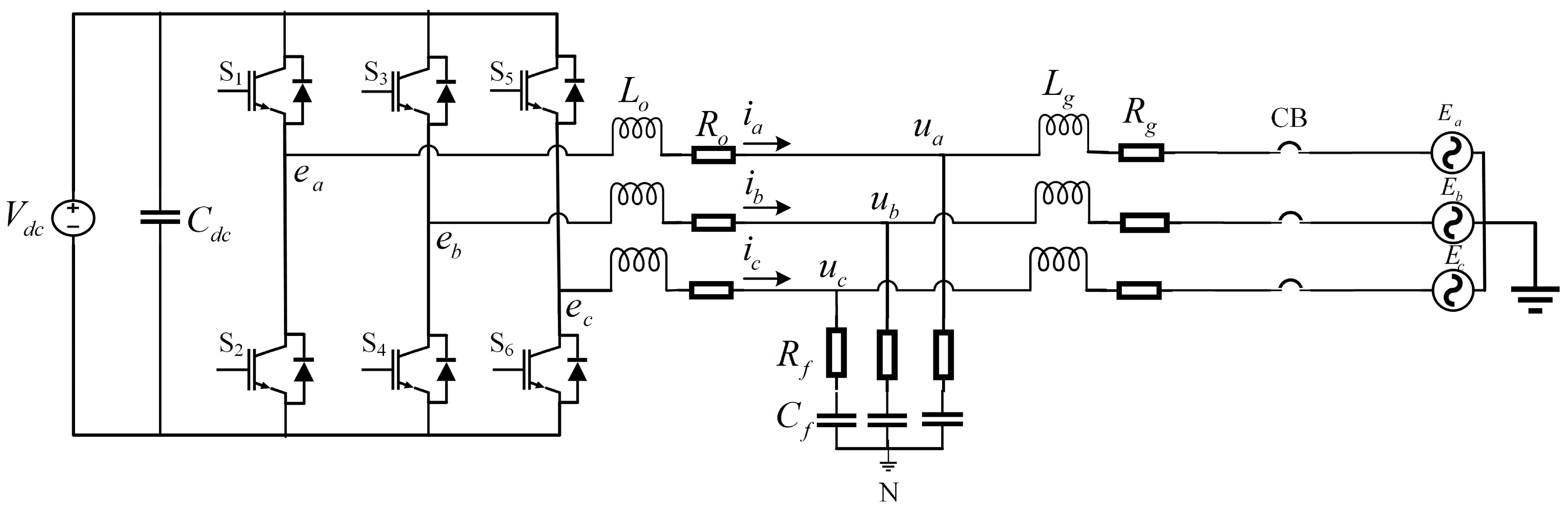
The most basic form of an inverter circuit that can be utilized in microgrids and controlled as a virtual synchronous generator to provide inertia and damping features is shown in Figure 1. The inverter’s DC side is fed by a DC voltage source that indicates the output voltage of a renewable energy source or a battery via a DC link. The grid is connected to the inverter output via an LCL filter. The electronic part of the inverter circuit represents the control system, which is used to control the power part. This circuit is clearly equivalent to the electrical section of the synchronous generator from a technical standpoint, where the neutral point voltage describes the three-phase bridge arm voltage, which represents the synchronous generator internal potential, and is the internal potential in phase a. The stator winding impedance of the synchronous generator is represented by and on the inverter side; thus, the impedance components of the rotor winding are described by and . The output voltage of inverter (capacitor voltage) indicates the synchronous generator’s three-phase terminal voltage, is phase a terminal voltage, and the inductance current can be used to describe the output current of the synchronous generator, where is the current through phase a.

Figure 1.
Power part of the inverter unit.
It is known that the LCL filter output causes reactive power loss; therefore, and will takevirtual synchronous generator output. According to the instantaneous power theory, the active and reactive power output can be determined using the electromotive force, and the inductance current [8,10,38], as
where , which represents the power angle. From Equation (4), the electrical torque can be derived:
Based on Equation (1), which represents the output voltage of the synchronous generator, the electromagnetic equation of virtual synchronous generator can be expressed as
where is VSG terminal voltage, is virtual armature resistance; is the virtual armature inductance, and both of them represent the components of the inverter output impedance, while is output current signal, and therefore
where is current angle. According to Equation (2), the part can be expressed as
in the above equation, is the virtual internal potential, is the virtual rotor flux which represents the virtual exciter output, and is the phase angle. Based on the voltage regulation equations, the expression for the reactive voltage and power droop control loop function, as shown in equation form, is as follows:
where is the system voltage reference value, is rated voltage, is the droop coefficient of voltage reactive power, is the reference command for reactive power, and is the actual reactive power output. Knowing that, the magnetic flux control circuit, as depicted in Figure 2 below, is responsible for generating the voltage amplitude in real synchronous generators.
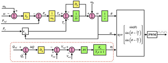
Figure 2.
VSG basic control structure.
Figure 2 shows a basic structure of the VSG control system, including the flux control circuit; it can be seen that the error generates by comparing the reference value of the voltage generated by the reactive power voltage in the droop control loop with the amplitude of the feedback measured output voltage . The error is sent to the virtual exciter after flowing through the PI controller. A low-pass filter is applied in virtual synchronous generators [8,24] for the following reasons:
- To mimic the synchronous generator’s flux weakness caused by the DC voltage applied to the rotor’s excitation circuit and the inductance of the rotor coil, which causes the stator to delay.
- A low-pass filter with a time constant can remove and filter high-frequency components of the output signals, which helps with the design of the backstepping controller based on ESO.
The design method is described in the next section.
3. Proposed Control Method
This section presents a backstepping controller with combined ESO, along with an analysis and a detailed design process based on the VSG core equations noted in the previous section.
3.1. Voltage Control Strategy
To design and integrate the backstepping controller into the flux control loop, the error signal generated by the droop control function links with the backstepping controller output signal, as depicted in Figure 3, which shows that the low-pass filter input signal is formulated as follows:
where is droop control function, and is the proposed output controller as compensator signal. The transfer function of the filter with a time constant has the following expression:
where is the gain of the low-pass filter, and is the low-pass filter time constant.
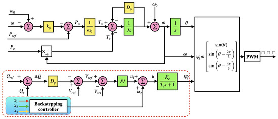
Figure 3.
Structure of VSG control circuit with compensating signal.
The dynamic change of power angle , angular frequency , and electrical torque are the system state variables that can be obtained as
where , and d represents uncertain bounded disturbance.
The model of the system (13) is simplified to execute the recommended control method by assuming that , and , which represents the system state variables. As a result, the following equation are used to summarize the model (13):
The system model (14) is a system with a bounded disturbance, d, that is unknown. A backstepping control strategy with second-order ESO is described and constructed in the section below to ensure the system’s stability and tracking performance. The system tracking errors can be defined by
where , and indicate the differences in variables between the reference and actual values, and is the reference value of .
1. The rotor angle dynamic error can be defined as
The Lyapunov function is defined as follows to stabilize the virtual rotor angle :
The derivative of selected function is given as follows:
In order to meet the system stability requirement, the appropriate power angle virtual control law is designed as follows:
The following equation is generated after substitution and incorporation:
where , and is a positive constant.
2. The mechanical angular velocity dynamic error can be presented as
The Lyapunov function should be chosen as follows to stabilize the angular velocity:
then, the following derivative can be obtained:
According to Equation (15), the relation between electrical torque dynamic error and the state variable can be described:
By substituting into Equation (23), the following result can be obtained:
To satisfy the stability condition, the angular velocity virtual control law must be developed in the following way to satisfy the initial condition:
then, the following result can be obtained:
where and are real numbers; thus, the quantity .
3. The electrical torque dynamic error can be defined as
The Lyapunov function is chosen as
The derivative of function can be defined as
To satisfy the stability condition, similarly, the term should be equal to or less than zero; thus, the virtual controller must be designed as follows:
then, the following result can be obtained:
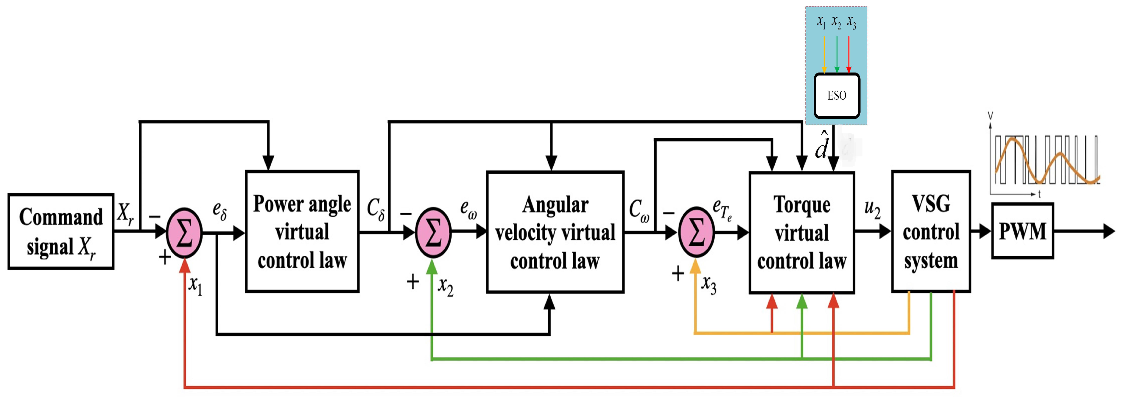
where , , and are positive constants; thus, the quantity . The structure of the designed controller is shown in Figure 4.

Figure 4.
Structure of backstepping controller combined ESO.
3.2. ESO Observer
In the above, Equation (31) contains externally uncertain disturbance, d. Thus, to ensure the system’s stability and to estimate the unpredictable external disruption, the nonlinear second-order ESO is designed as follows:
where is the observation of the state variable in the system (14), and are observer gain settings, and the function is given by
where is the observer error, and is a constant in the interval (0, 1). Furthermore, is the length of the interval of the linear segment [32,37,39]. To ensure the stability of the observer described by Equation (33), the following assumptions must be satisfied:
Assumption 1.
When satisfies the condition , then the function , then
When the system goes into the steady state, the derivative of and is almost close to zero:
Result: when the part is established, it can be obtained that is close to , and is close to d.
Assumption 2.
When satisfies the condition , then the function , and
When the system goes into the steady state, the derivatives of and are almost close to zero.
Result: Likewise, when the part is formed, it can be obtained that is close to , and is close to d.
From the above analysis, we conclude that the stability of the system based on low-order ESO can be ensured when the following conditions are satisfied: and . For more equations details, please see Appendix A.
4. Simulation Results
This section presents simulation results for the VSG-controlled inverter to demonstrate the suggested methodology’s practicality. For verification and validation of the suggested control strategy, the model is developed in the MATLAB/Simulink environment R2018a. In order to move closer to the actual system operation situation, the simulation experiments are conducted for three cases based on the microgrid configuration of Figure 1. The cases include two types of load variation disturbances and transition processes (grid connection and disconnection); the simulation time is 1.2 s for each case. The parameters for the system model during the simulation tests are chosen as listed in Table 1 and Table 2. Moreover, based on the Lyapunov stability theory, the appropriate , , and are selected to achieve the rapid stability of the system as follows: , , and . Furthermore, the parameters for the second-order extended state observer were selected as follows: , , , and

Table 1.
Microgrid parameters.
Table 2.
The parameters of the VSG controller.
4.1. Load Variation Disturbances
The variation of the load demand influences the microgrid output, so the microgrid control shall interact with such disturbances to provide stable operation and acceptable performance. The simulation process in these cases is based on Figure 1, which operates in an isolated operation mode.
4.1.1. Case-1
At t = 0 s, the inverter provides active power to the supplied 7 kW local load. Then, when t = 0.4 s, the load suddenly increased to 10 kW; at t = 0.8 s, the 3 kW is removed. The simulation results of this case are shown in the following figures: Figure 5 demonstrates the active power variation result, Figure 6 shows the frequency response, and Figure 7 and Figure 8 depict the variation of three-phase voltage and current, respectively. The system tracking errors are illustrated in Figure 9.
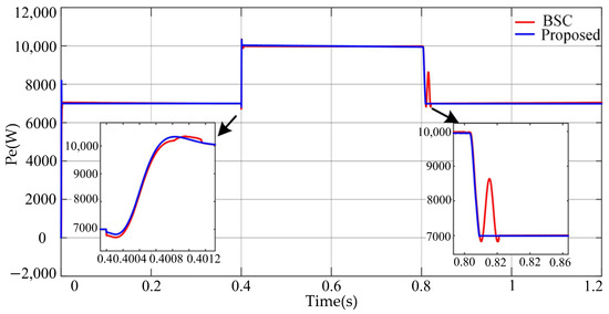
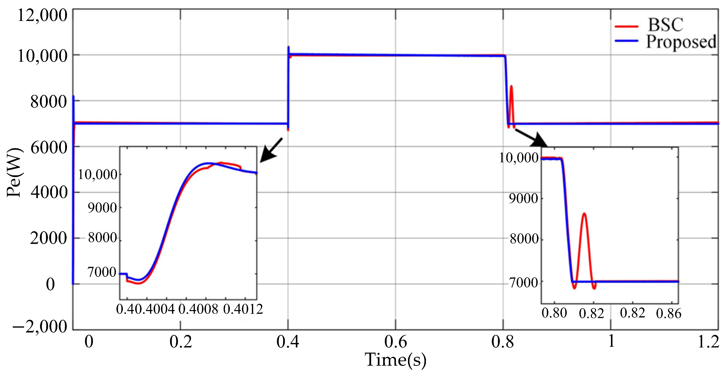
Figure 5.
Active power variation result of case-1.
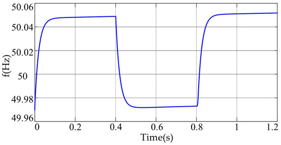
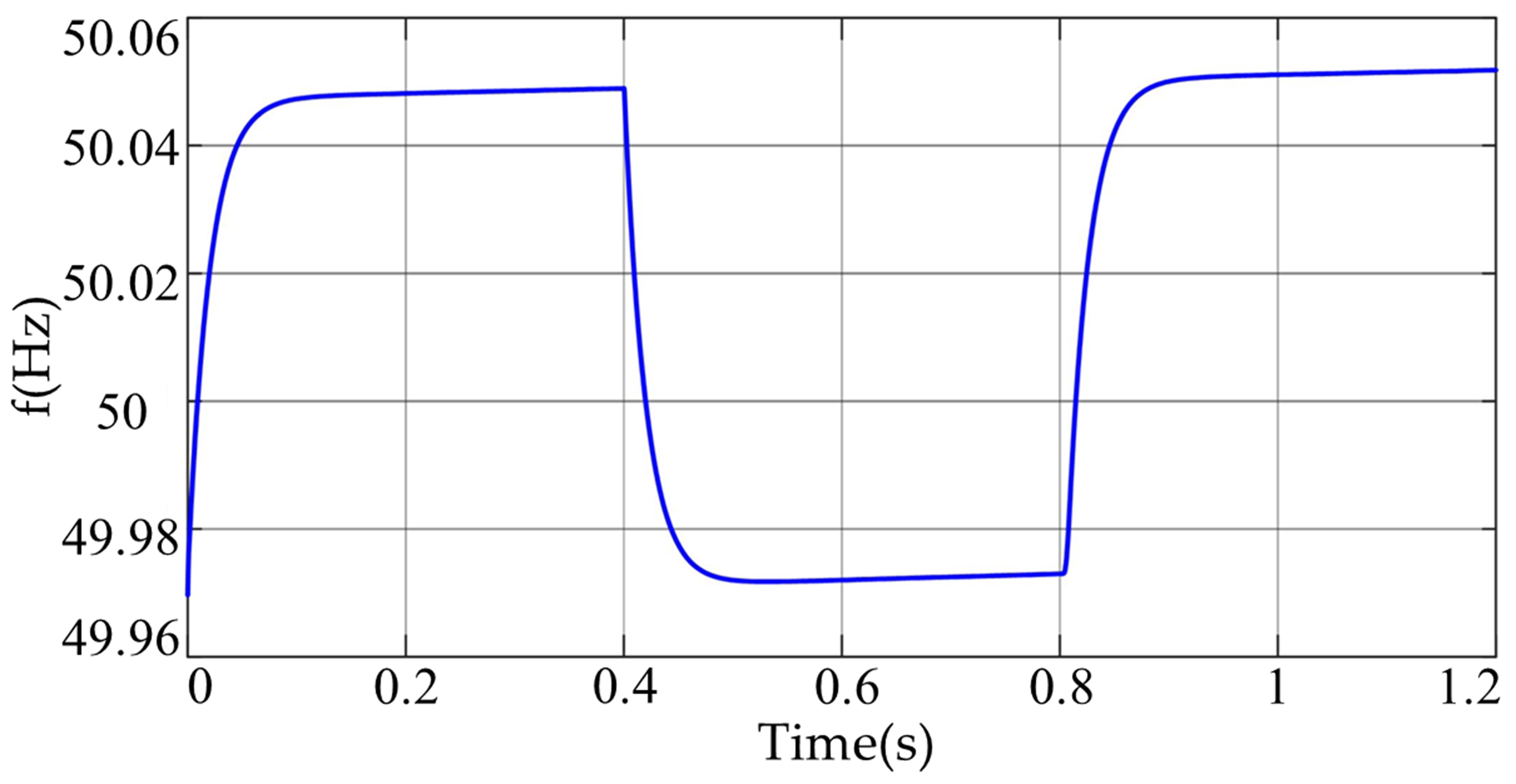
Figure 6.
Frequency variation result of case-1.
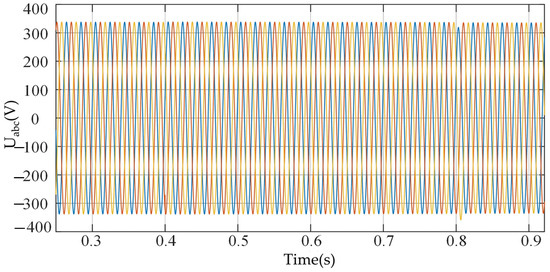
Figure 7.
Variation of three-phase voltage in case-1.
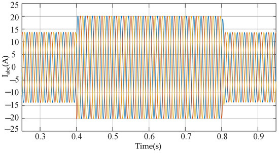
Figure 8.
Variation of three-phase current in case-1.

Figure 9.
Active power variation result of case-2.
4.1.2. Case-2
In this case, the system operates stably and supplies 10 kW load demand initially. At t = 0.4 s, 3 kW active power was removed; then, when t = 0.8 s, 3 kW load was added again. Similarly, the simulation results of this case are illustrated as follows: Figure 10 depicts the active power variation result, Figure 11 shows the frequency variation result, Figure 12 illustrates the three-phase voltage situation, Figure 13 exhibits the three-phase current variation, and Figure 14 depicts the system tracking errors of case-2.
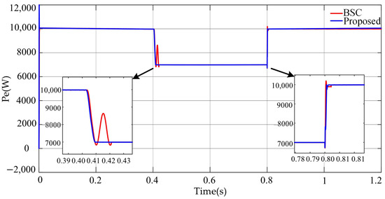
Figure 10.
Frequency variation result of case-2.
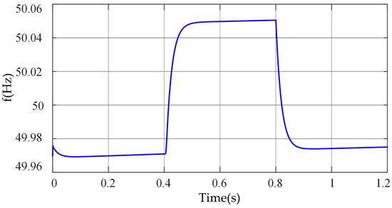
Figure 11.
Three-phase voltage variation situation result of case-2.
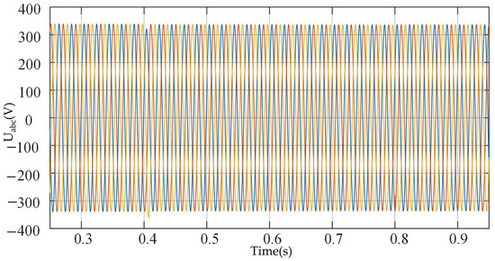
Figure 12.
Three-phase current variation situation result of case-2.
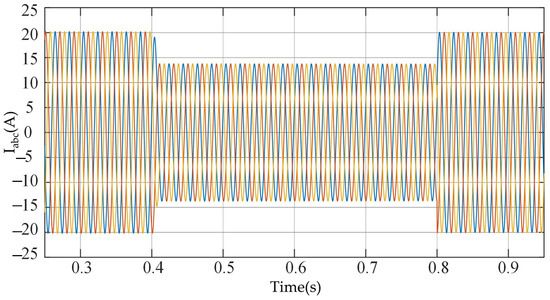
Figure 13.
System tracking errors , , and of case-2.
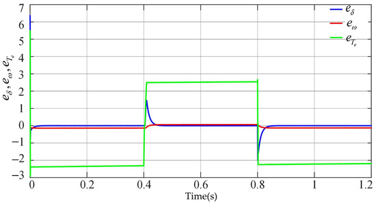
Figure 14.
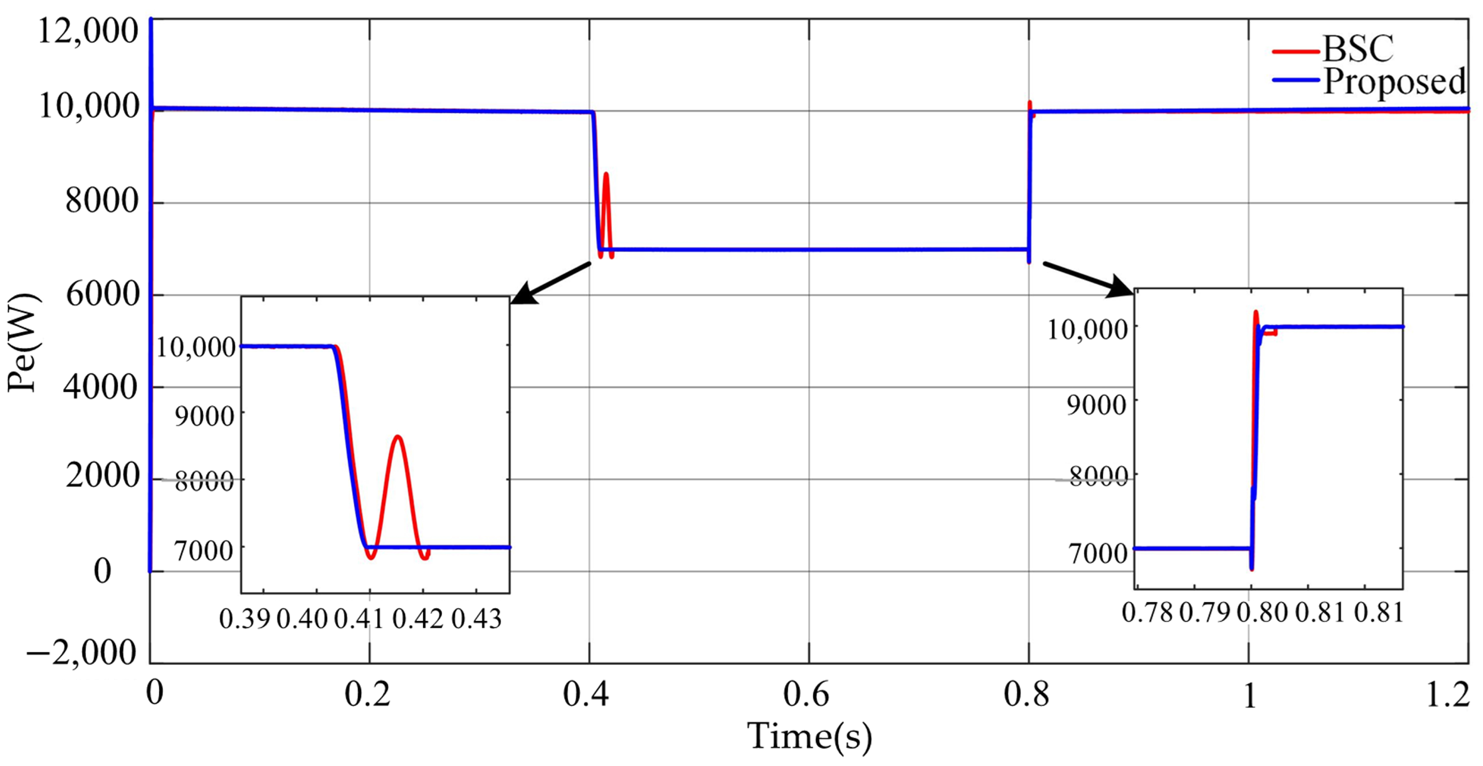
Output power result during the transition process.
4.2. Transition Process
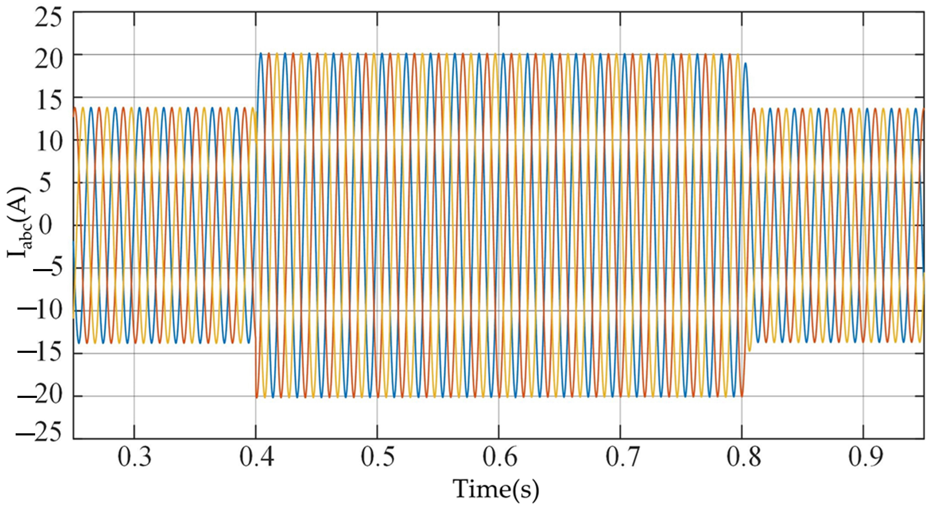
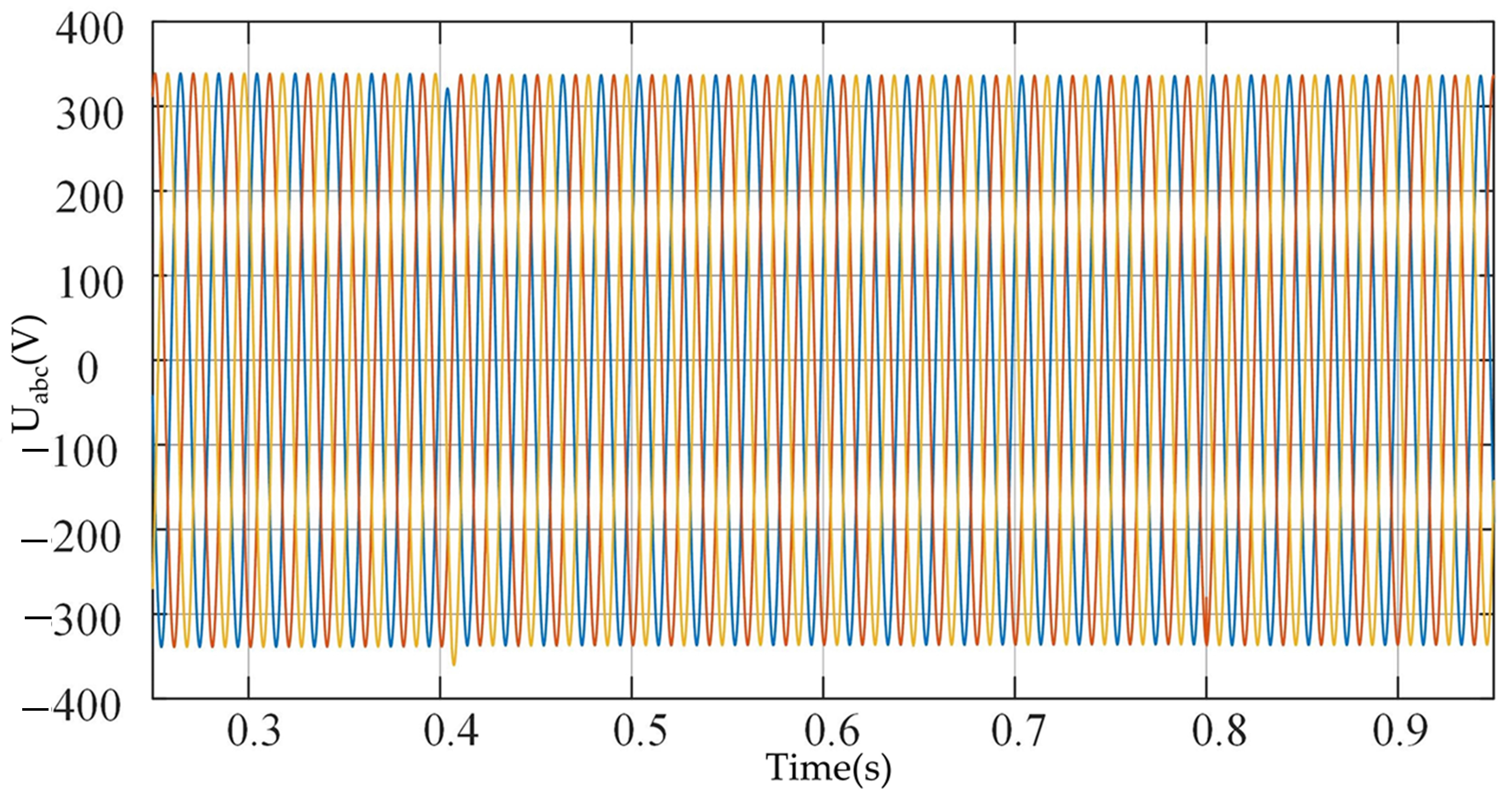
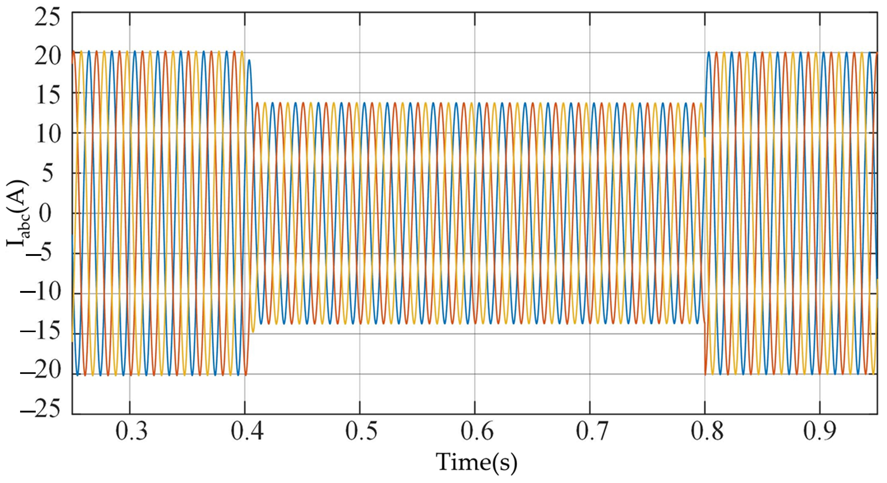
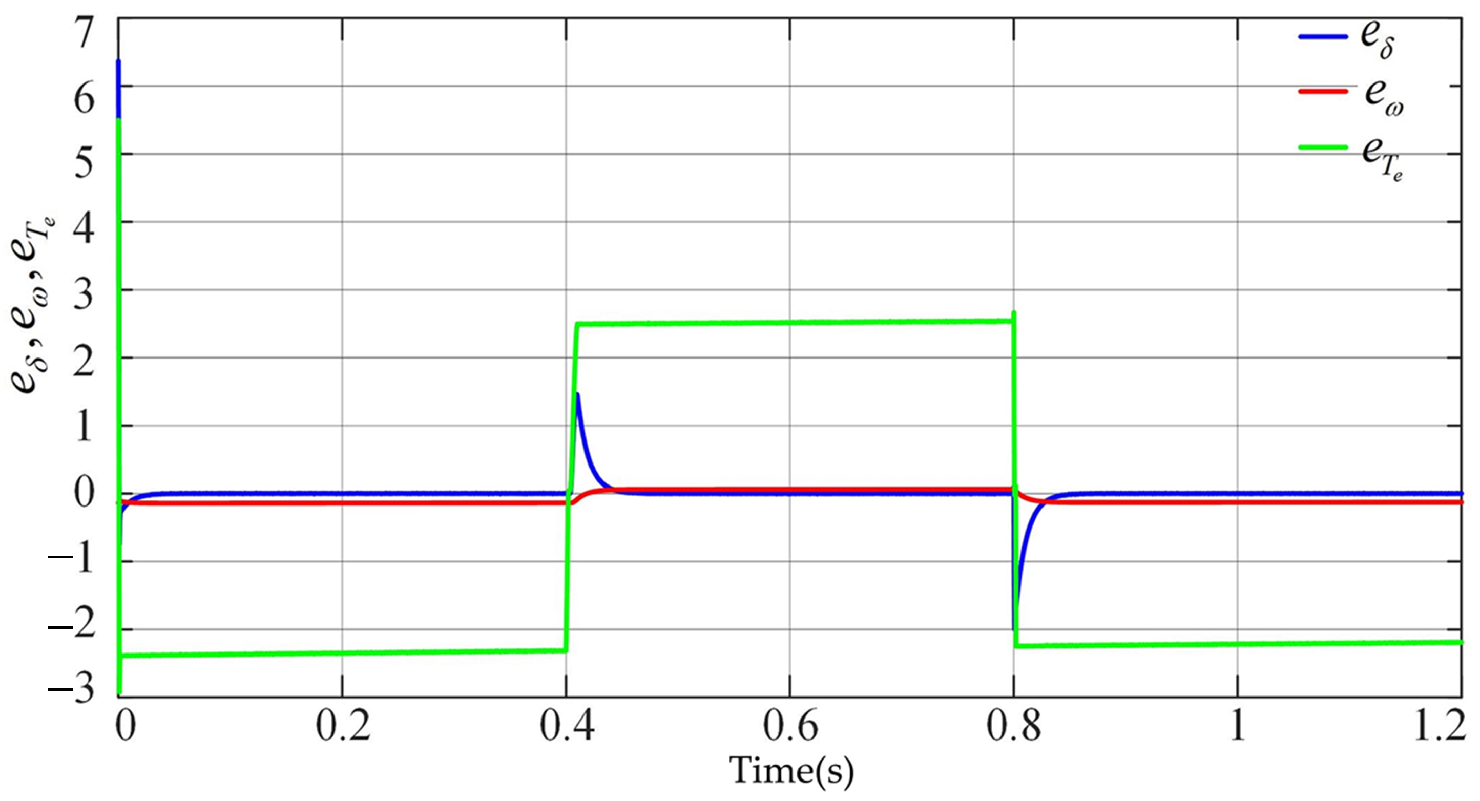
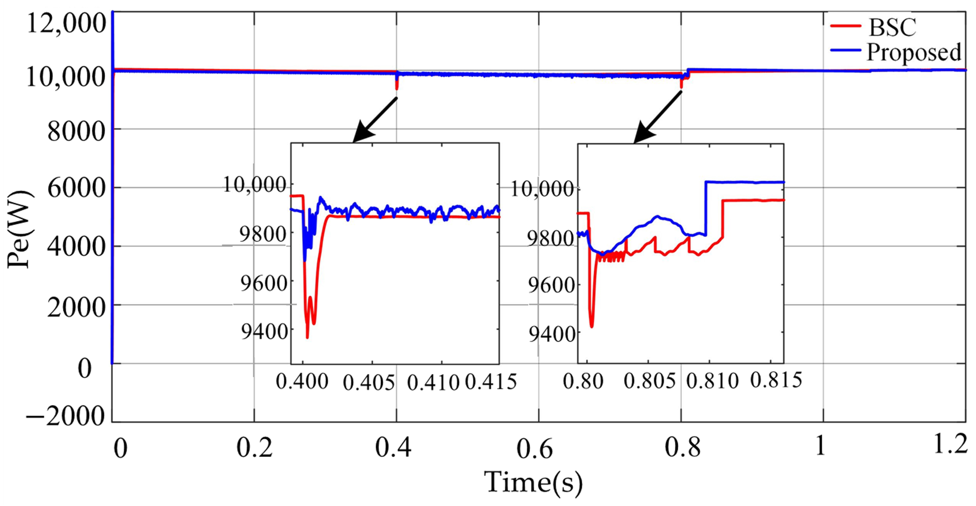
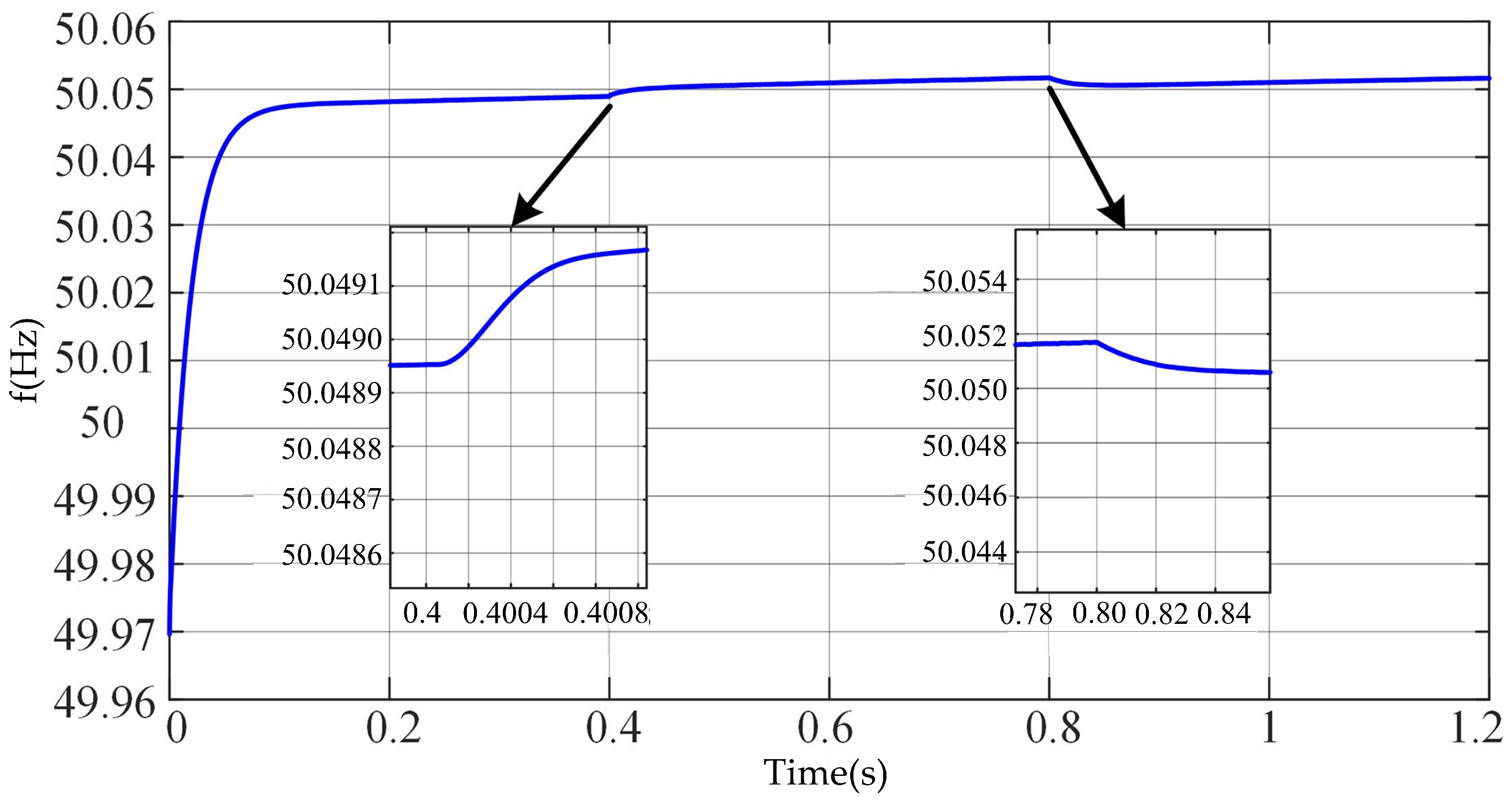
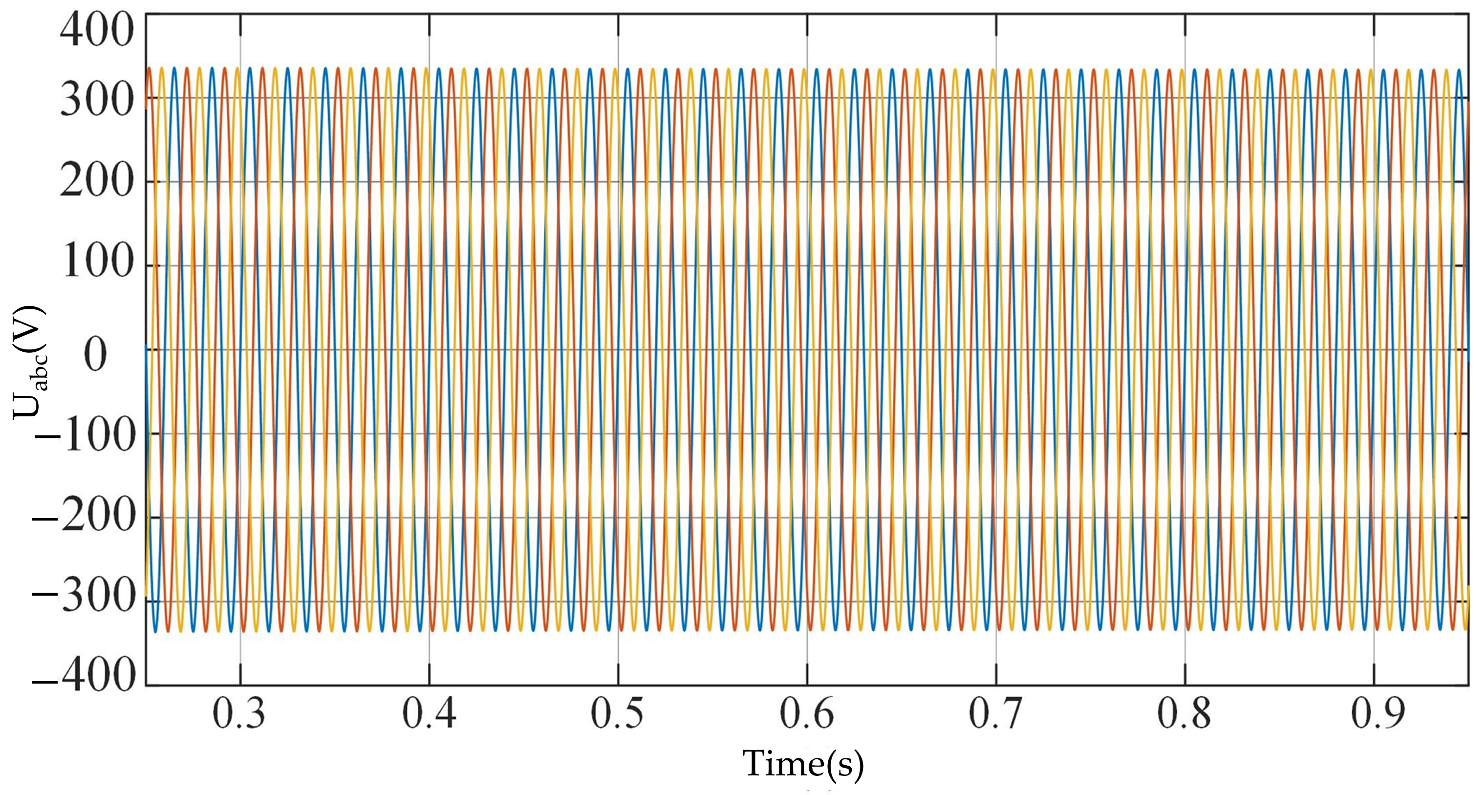
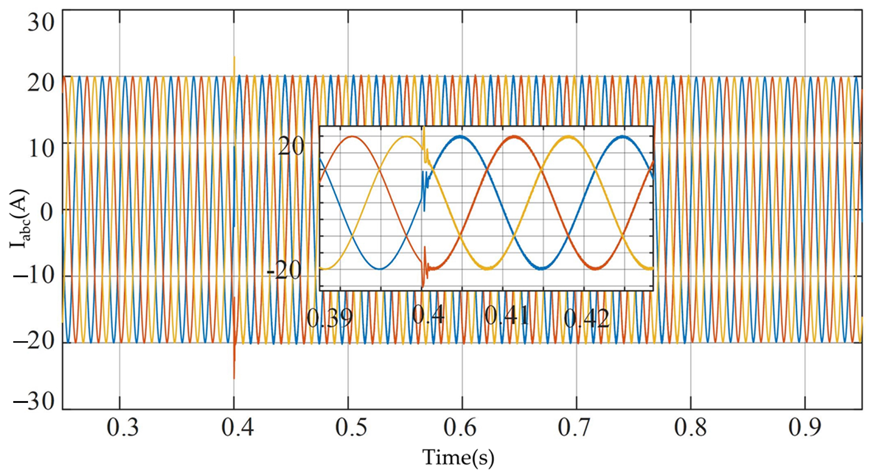
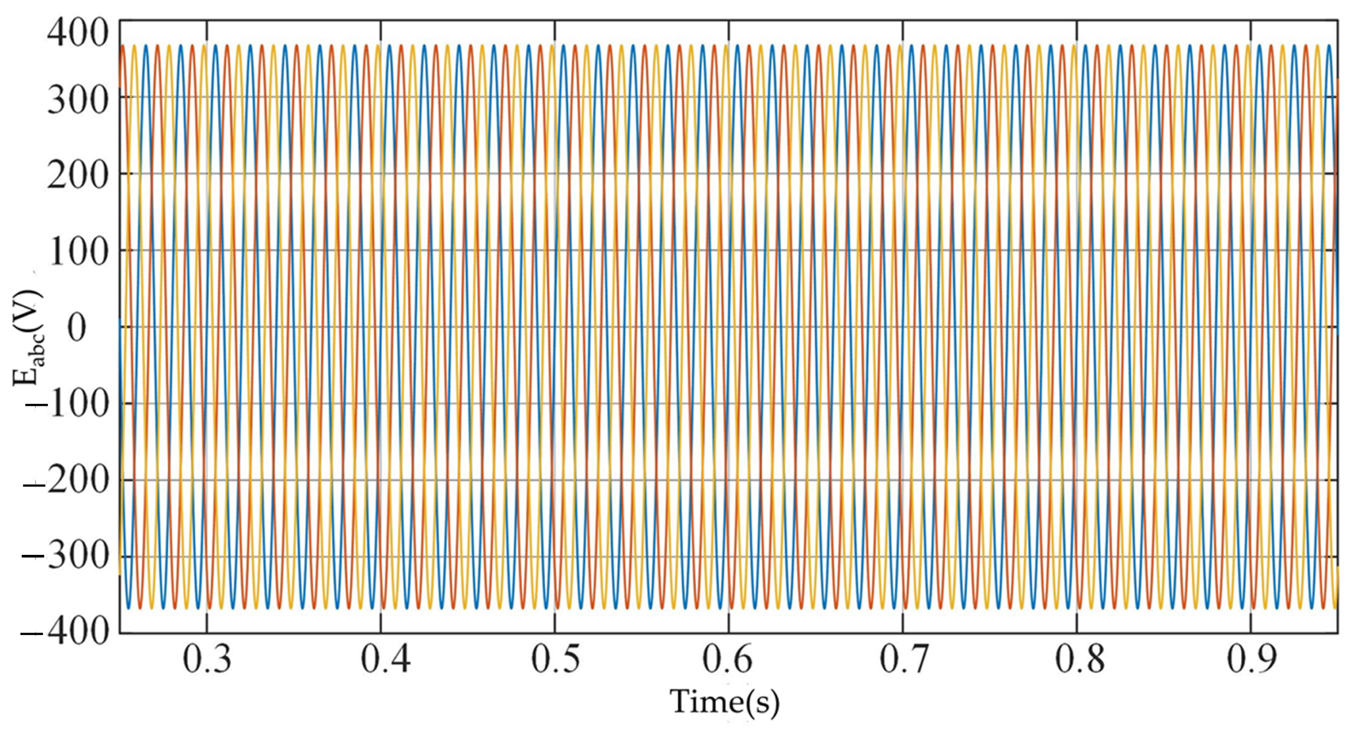
The connection and disconnection process also affects the system’s output parameters, so testing the controller’s robustness in such conditions is necessary to ensure stable operation. Therefore, in this case, the simulation results demonstrate the control performance of the proposed controller during the system transfer from the off-grid to the grid-connected. The system presented in Figure 1 works in off-grid mode first, and the rated power is 10 kW of active power. Because the grid is running correctly and there is no failure condition, the system needs to be connected to the grid, and CB is closed at t = 0.4 s. Due to sudden failure on the grid side at t = 0.8 s, CB opens again. In other words, when t = 0.8 s, the system needs to transfer from grid connection operation mode to island operation mode. The corresponding simulation results are depicted in Figure 15, Figure 16, Figure 17, Figure 18, Figure 19, Figure 20, Figure 21, Figure 22, Figure 23 and Figure 24.
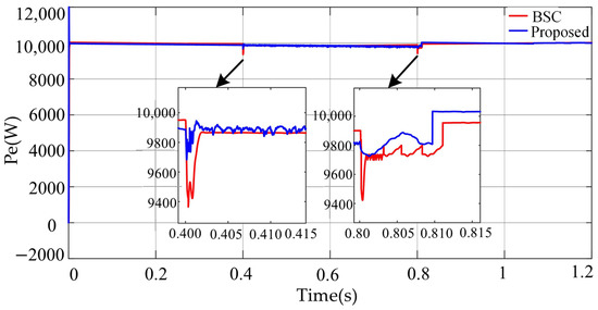
Figure 15.
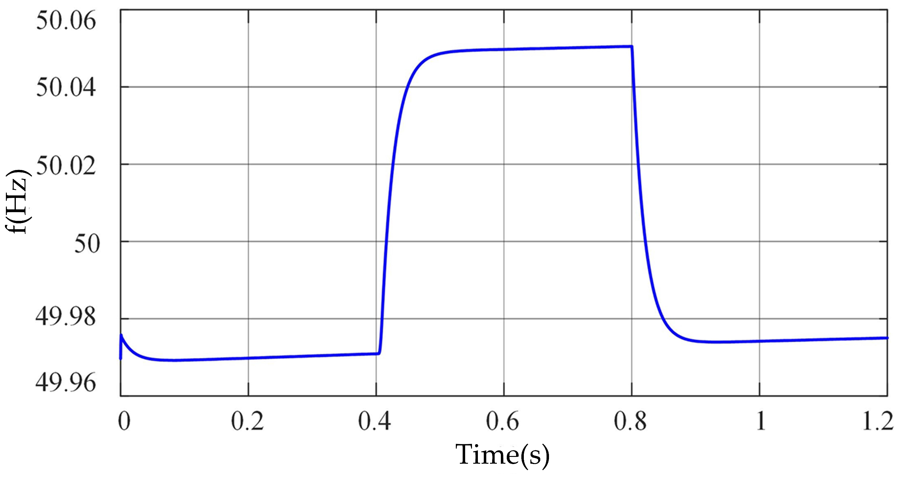
System frequency response result during the transition process.

Figure 16.
Three-phase voltage variation result during the transition process.
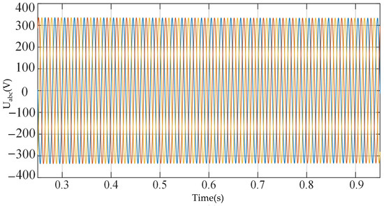
Figure 17.
Three-phase current variation situation result during the transition process.
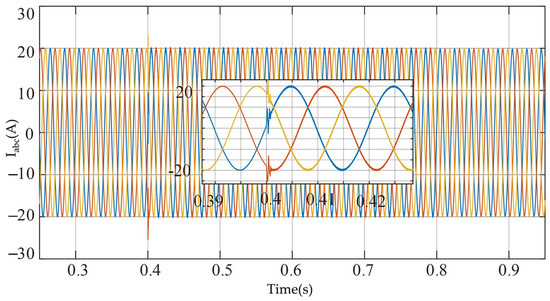
Figure 18.
Grid voltage variation during the transition process.
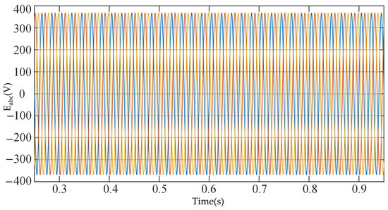
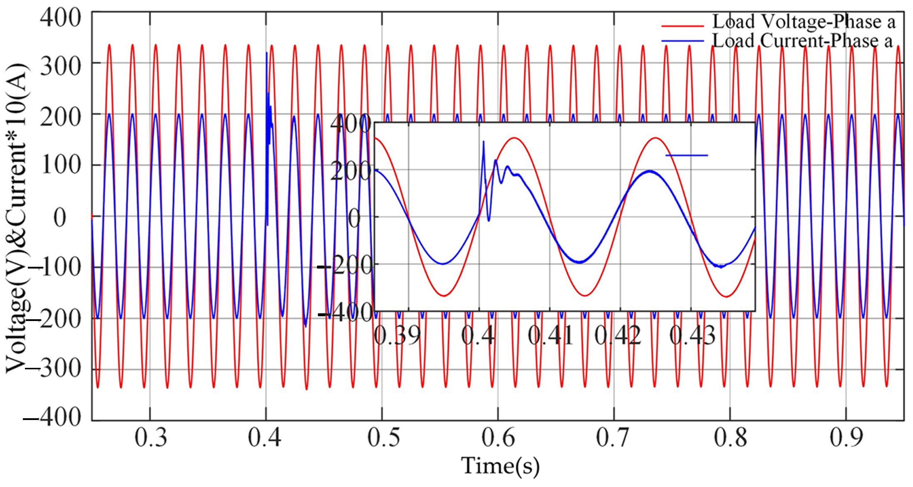
Figure 19.
Variation of load voltage and current (phase-a) during the transition process.
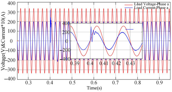
Figure 20.
Output voltage response during the transition process.
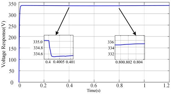
Figure 21.
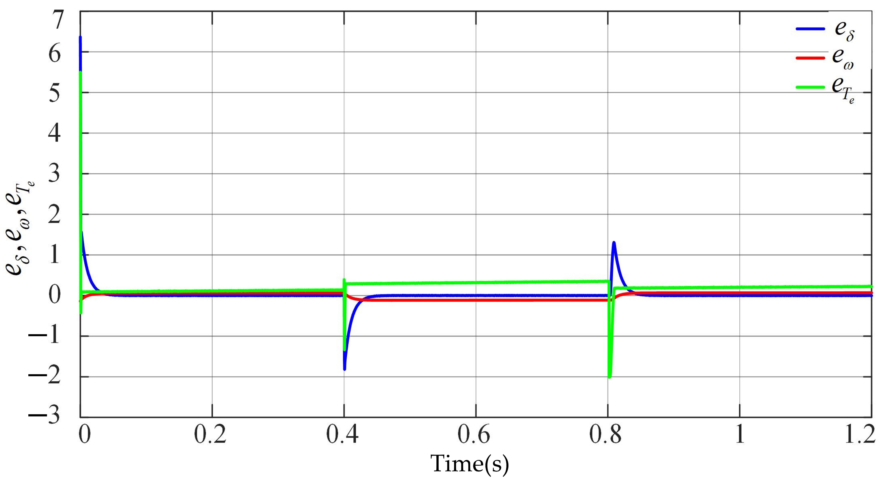
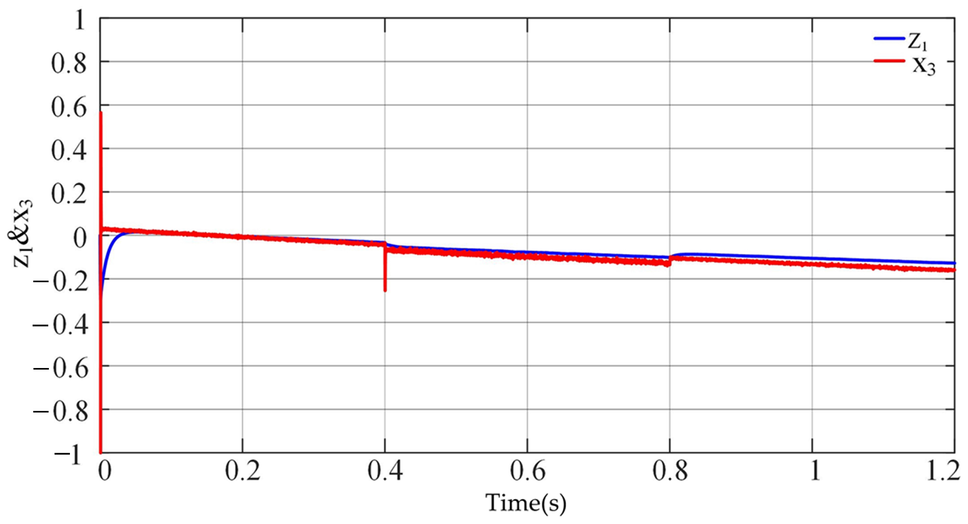
System tracking errors , , and .
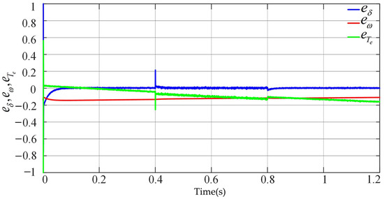
Figure 22.
System state variable and estimated value .
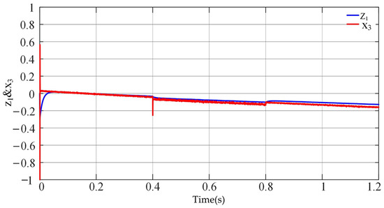
Figure 23.
Uncertain disturbance d and predicted disturbance .
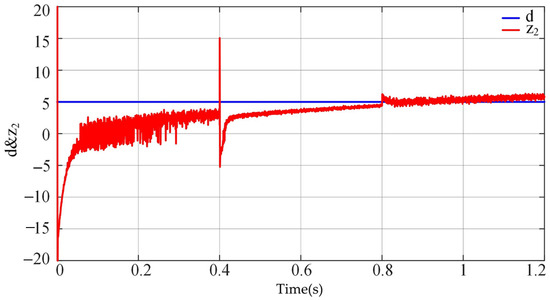
Figure 24.
System tracking errors , , and in case-1.
5. Discussion
The active power output effects are the main point of discussion and analysis, together with other parameters representing frequency, voltages, and currents, in cases of off-grid and transfer from islanding mode to grid connection modes.
5.1. Load Variation Disturbances
5.1.1. Case-1
Figure 5 depicts the active power variation result of simulation under both the proposed control strategy and BSC. It can be understood that the active power can easily and smoothly meet the desired value with the minor amplitude fluctuation at the beginning when t = 0 s, then returned to its target output. Due to adding a 3 kW load at t = 0.4 s, the load variation disturbance causes a sudden power imbalance between the demand and output power; this process leads to a slight fluctuation in the active power to 6871 W, then increases immediately to 10,333 W. Results of the suggested control technique show that the value of the active power is returned to the expected value. At the same time, the BSC oscillates between 6710 W–10350 W at 0.4 s and 8640 W–6830 W for 0.021 s after removing the added load at t = 0.8 s. No changes affect the system output power performance under the proposed control method when the 3 kW load is switched off at t = 0.8 s. Due to load increasing, the frequency decreases by about 0.075 Hz, as shown in Figure 6, which illustrates the frequency variation during the sudden load increase and decrease simulation result, where it is evident that the system frequency varies between 49.97 Hz and 50.05 Hz; this range remains within an acceptable value. Figure 7 and Figure 8 show the system output voltages and currents in three phases, respectively. The voltage and current waveforms can easily remain unchanged when the system is suddenly loaded under the suggested control technique. Figure 9 shows the tracking errors of the system state variables during the step load change, which are almost zero.
5.1.2. Case-2
Figure 10 demonstrates active power variation throughout simulation testing under the proposed control approach and BSC; it is evident that the active power curve of the proposed control strategy can provide good transient responses with no fluctuation when the load is reduced at t = 0.4 s, while the maximum fluctuation of the BSC is between 6830 W–8650 W during the interval 0.4–0.421 s. However, when the load increases again, the active power drops to 6730 W at t = 0.8 s, then immediately climbs to 10,030 W before returning to its steady state under the recommended control mechanism; simultaneously, the oscillation in the case of BSC ranges between 6709.8 W–10,192.4 W. Figure 11 shows the frequency variation result of case-2; according to this result, the system operates at a frequency lower than the reference frequency; when 3 kW is removed, the frequency increases by 0.078 Hz due to load decrease until t = 0.8 s, and when the load is added again the frequency decreases by about 0.025 Hz. Figure 12 and Figure 13 represent the system output voltage and current waveforms, respectively. It is clear that during this case, the three-phase waves of voltage and current also remain unchanged, which is a unique feature of this control approach. Figure 14 represents the system tracking errors of the state variables during the load changing in case-2.
According to the previous simulation experiment results, for VSG working in an off-grid system, under the proposed strategy, the oscillation amplitude of the system output parameters caused by load fluctuation is mostly minor, and the time of restoration to stability is fast, which indicates satisfactory obtained results.
5.2. Transition Process
Figure 15 demonstrates the active power output result at the moment of grid connecting for both the suggested control approach and BSC. The curves show that due to the power angle needing to be restored, the active power decreases to 9700 W under the recommended method and 9400 W under BSC at t = 0.4 s, and then quickly returns to the desired value until the system disconnects at t = 0.8 s. The system is exposed to a slight oscillation for a short period and then disappears due to the proposed control mechanism at the moment of disconnecting, while in the case of BSC, the output power drops to 9420 W and then returns to a stable state at the moment of disconnecting. As it can be understood from the simulation result introduced by Figure 15, the proposed controller developed in this paper can offer a more excellent stable operation and provides smoother output power during transient actions than BSC, particularly in the 0.4 s and 0.8 s intervals. The fluctuation range is also smaller than the BSC, and the control performance is more acceptable.
Figure 16 shows the frequency variation during the off-grid and grid connection simulation test. It can be seen that the system frequency is stable and remains close to the reference value with not too much change; this result reflects the performance of the suggested controller for improving system stability. Figure 17, Figure 18, Figure 19, Figure 20 and Figure 21 represent the system output parameters of three-phase voltage, three-phase current, grid voltage, load voltage and current, and voltage response variation, respectively. It can be noted that the suggested control method’s oscillation ranges during the transfer from islanding to grid connecting and vice versa are very small, resulting in a smooth switching process without any disturbing deviations or causing voltage transients. Nevertheless, the three-phase current waveforms in Figure 18 have a relatively large deviation when the CB is switched on at t = 0.4 s, which fluctuates between 23A and −25.3A and maintains 0.006 s before returning to the desired value by the proposed strategy. When there is a more significant gap between the grid voltage and the VSG output voltage, the inpouring current will also grow, and hence there will be an increase in power variation and system instability. The effect of inpouring current fluctuation on the output power is illustrated in Figure 15. The system tracking errors, state variable with estimated value , and uncertain disturbance d with predicted disturbance during this simulation experiment test are shown in Figure 23 and Figure 24, respectively. The system tracking errors of curves in Figure 22 are close to zero, which indicates the stability process. Knowing that, the error can monitor changes and adapt the system more precisely to achieve a stable operation. Figure 23 and Figure 24 show that the developed ESO can conduct effective dynamic compensation for the uncertain disturbance term and efficient tracking, and this validates what was achieved in the analysis and discussed in Section 3. These results illustrate the extent to which the system under the proposed controller can guarantee stability and faster response, and it has tremendous practical utility. For more verification of the usefulness of this method, Table 3 compares the results obtained in this work with other recently proposed control strategies for improving the microgrid stability objective.
Table 3.
Comparison of various VSG strategies for stability improvement with the proposed method.
6. Conclusions
In response to low inertia and damping properties issues in a microgrid system, the system shows a low output impedance, leading to instability, particularly in the transition process. This paper designs a new control method that combines backstepping control with an extended state observer to improve the operational performance of the proposed inverter topology. It enables a seamless transition between off-grid and grid-tied; thereby, the overall control performance of the microgrid will improve. The linear control part, which represents the rotor swing equations, is presented based on the synchronous generator model. Then, the nonlinear controller is constructed, and controller stability is proved using the Lyapunov function.
The simulation results affirm the adequacy of the proposed control technique so that the microgrid system’s stability and dynamic performance are verified. Moreover, uncertainties, including external disturbances and tracking errors, are taken into consideration and predicted using the proposed extended state observer with high accuracy performance. Theoretical evaluation shows that the developed controller for the virtual synchronous generator can reduce the power oscillation at the moment of load demand change and provide a seamless transition between off-grid and grid-tied compared with traditional backstepping control, which validates the greatest control performance under the suggested control technique for the microgrid system.
In future work, we will build an experiment platform of a small microgrid, including multi-VSGs, to verify our suggested controller’s practical effectiveness.
Author Contributions
Conceptualization, S.I.A.H., Y.Z. (Yun Zeng) and J.Q.; methodology, S.I.A.H. and J.Q.; software, S.I.A.H., Y.Z. (Yidong Zou) and D.T.; validation, S.I.A.H. and J.Q.; writing: original draft preparation, S.I.A.H.; writing: review and editing, Y.Z. (Yidong Zou) and D.T.; supervision, Y.Z. (Yun Zeng) and J.Q.; funding acquisition, Y.Z. (Yun Zeng). All authors have read and agreed to the published version of the manuscript.
Funding
This research was funded by the National Natural Science Foundation of China, grant numbers (51869007, 52079059).
Conflicts of Interest
The authors declare no conflict of interest.
Abbreviations
The following abbreviations are used in Table 3, Section 5:
| ATSMC | Adaptive Terminal Sliding Mode Control |
| OPIC | Optimized Proportional-Integral Controller |
| ISMBC | Integral Sliding Mode Backstepping Control |
| ACBC | Adaptive Command-Filter Backstepping Control |
| ATSMBSC | Adaptive Terminal Sliding Mode Backstepping Control |
| FIS | Fuzzy Inference System |
Appendix A
The following derivations are used in this manuscript:
The observer dynamics error:
References
- Magdy, G.; Bakeer, A.; Nour, M.; Petlenkov, E. A new virtual synchronous generator design based on the SMES system for frequency stability of low-inertia power grids. Energies 2020, 13, 5641. [Google Scholar] [CrossRef]
- Abdalla, M.A.A.; Min, W.; Mohammed, O.A.A. Two-stage energy management strategy of EV and PV integrated smart home to minimize electricity cost and flatten power load profile. Energies 2020, 13, 6387. [Google Scholar] [CrossRef]
- Nogami, S.; Yokoyama, A.; Daibu, T.; Hono, Y. Virtual synchronous generator model control of PV for improving transient stability and damping in a large-scale power system. Electr. Eng. Jpn. 2019, 208, 21–28. [Google Scholar] [CrossRef]
- Badal, F.R.; Das, P.; Sarker, S.K.; Das, S.K. A survey on control issues in renewable energy integration and microgrid. Prot. Control Mod. Power Syst. 2019, 4, 8. [Google Scholar] [CrossRef]
- Kamel, R.M.; Chaouachi, A.; Nagasaka, K. Detailed analysis of microgrid stability during islanding mode under different load conditions. Engineering 2011, 3, 508. [Google Scholar] [CrossRef]
- Zeng, Y.; Qian, J.; Yu, F.; Mei, H.; Yu, S. Damping Formation Mechanism and Damping Injection of Virtual Synchronous Generator Based on Generalized Hamiltonian Theory. Energies 2021, 14, 7082. [Google Scholar] [CrossRef]
- Chen, M.; Zhou, D.; Blaabjerg, F. Modelling, implementation, and assessment of virtual synchronous generator in power systems. J. Mod. Power Syst. Clean Energy 2020, 8, 399–411. [Google Scholar] [CrossRef]
- Yang, C.; Yang, F.; Xu, D.; Huang, X.; Zhang, D. Adaptive command-filtered backstepping control for virtual synchronous generators. Energies 2019, 12, 2681. [Google Scholar] [CrossRef]
- Rehman, H.U.; Yan, X.; Abdelbaky, M.A.; Jan, M.U.; Iqbal, S. An advanced virtual synchronous generatorcontrol technique for frequency regulation of grid-connected PV system. Int. J. Electr. Power Energy Syst. 2021, 125, 106440. [Google Scholar] [CrossRef]
- Zhang, X.; Gao, Q.; Guo, Z.; Zhang, H.; Li, M.; Li, F. Coordinated control strategy for a PV-storage grid-connected system based on a virtual synchronous generator. Glob. Energy Interconnect. 2020, 3, 51–59. [Google Scholar] [CrossRef]
- Bevrani, H.; Ise, T.; Miura, Y. Virtual synchronous generators: A survey and new perspectives. Int. J. Electr. Power Energy Syst. 2014, 54, 244–254. [Google Scholar] [CrossRef]
- Alipoor, J.; Miura, Y.; Ise, T. Stability assessment and optimization methods for a microgrid with multiple VSG units. IEEE Trans. Smart Grid 2016, 9, 1462–1471. [Google Scholar] [CrossRef]
- Liu, J.; Miura, Y.; Ise, T. A novel oscillation damping method of virtual synchronous generator control without PLL using pole placement. In Proceedings of the 2018 IEEE International Power Electronics Conference, Niigata, Japan, 20–24 May 2018. [Google Scholar]
- Yu, Y.J.; Cao, L.K.; Zhao, X. A novel control strategy of virtual synchronous generator in island microgrids. Syst. Sci. Control Eng. 2018, 6, 136–145. [Google Scholar] [CrossRef]
- Mohamed, M.M.; El Zoghby, H.M.; Sharaf, S.M.; Mosa, M.A. Optimal virtual synchronous generator control of battery/supercapacitor hybrid energy storage system for frequency response enhancement of photovoltaic/diesel microgrid. J. Energy Storage 2022, 51, 104317. [Google Scholar] [CrossRef]
- Zhou, B.; Meng, L.; Yang, D.; Ma, Z.; Xu, G. A Novel VSG-Based Accurate Voltage Control and Reactive Power Sharing Method for Islanded Microgrids. Sustainability 2019, 11, 6666. [Google Scholar] [CrossRef]
- Lalitha, M.P.; Anupama, S.; Faizal, K.M. Fuzzy logic controller for parallel inverters in microgrids using virtual synchronous generator control. In Proceedings of the IEEE International Conference on Energy, Communication, Data Analytics and Soft Computing (ICECDS), Chennai, India, 1–2 August 2017. [Google Scholar]
- Li, W.; Xie, J.; Zhang, M.; Guo, C. Adaptive damping control strategy of virtual synchronous generator based on fuzzy control. In Proceedings of the IOP Conference Series, Zamosc, Poland, 25–27 November 2021. [Google Scholar]
- Karimi, A.; Khayat, Y.; Naderi, M.; Dragicevic, T.; Mirzaei, R.; Blaabjerg, F.; Bevrani, H. Inertia response improvement in AC microgrids: A fuzzy-based virtual synchronous generator control. IEEE Trans. Power Electron. 2019, 35, 4321–4331. [Google Scholar] [CrossRef]
- Karimi, A.; Jafarian, Y.; Bevrani, H.; Mirzaei, R. Frequency response improvement in microgrids:afuzz-based virtual synchronous generator approach. Int. J. Ind. Electron. Control Optim. 2020, 3, 147–158. [Google Scholar]
- Kerdphol, T.; Watanabe, M.; Hongesombut, K.; Mitani, Y. Self-adaptive virtual inertia control-based fuzzy logic to improve frequency stability of microgrid with high renewable penetration. IEEE Access 2019, 7, 76071–76083. [Google Scholar] [CrossRef]
- Zhang, L.; Zheng, H.; Wan, T.; Shi, D.; Lyu, L.; Cai, G. An integrated control algorithm of power distribution for islanded microgrid based on improved virtual synchronous generator. IET Renew. Power Gener. 2021, 15, 2674–2685. [Google Scholar] [CrossRef]
- Lin, S.; Lin, L.; Wen, B. A Voltage Control Strategy of VSG Based on Self-Adaptive Inertia Coefficient and Droop Coefficient. Math. Probl. Eng. 2021, 2021, 5567826. [Google Scholar] [CrossRef]
- Zhang, G.; Yang, J.; Wang, H.; Cui, J. Presynchronous Grid-Connection Strategy of Virtual Synchronous Generator Based on Virtual Impedance. Math. Probl. Eng. 2020, 2020, 3690564. [Google Scholar] [CrossRef]
- Liu, J.; Miura, Y.; Ise, T. Fixed-parameter damping methods of virtual synchronous generator control using state feedback. IEEE Access 2019, 7, 99177–99190. [Google Scholar] [CrossRef]
- Li, J.; Wen, B.; Wang, H. Adaptive virtual inertia control strategy of VSG for microgrid based on improved bang-bang control strategy. IEEE Access 2019, 7, 39509–39514. [Google Scholar] [CrossRef]
- Li, L.; Li, H.; Tseng, M.L.; Feng, H.; Chiu, A.S. Renewable energy system on frequency stability control strategy using virtual synchronous generator. Symmetry 2020, 12, 1697. [Google Scholar] [CrossRef]
- Chen, X.; Zhang, Y.; Dong, J.; Mao, X.; Chen, J.; Wen, B.; Zhang, Z. A Novel Pre-Synchronization Control for Grid Connection of Virtual Synchronous Generator. Elektron. Ir Elektrotechnika 2020, 26, 25–31. [Google Scholar] [CrossRef]
- Lan, Y.H. Backstepping control with disturbance observer for permanent magnet synchronous motor. J. Control Sci. Eng. 2018, 2018, 4938389. [Google Scholar] [CrossRef]
- Teng, Q.; Xu, D.; Yang, W.; Li, J.; Shi, P. Neural network-based integral sliding mode backstepping control for virtual synchronous generators. Energy Rep. 2021, 7, 1–9. [Google Scholar] [CrossRef]
- Dou, Z.; Tang, L.; Sun, Y.; Zhang, C.; Yang, W.; Xu, D. Prescribed Performance-Based Adaptive Terminal Sliding Mode Control for Virtual Synchronous Generators. Math. Probl. Eng. 2022, 2022, 5742759. [Google Scholar] [CrossRef]
- Deng, G.; Cheng, L.; Yang, B. Adaptive optimizing control for nonlinear synchronous generator system with uncertain disturbance. Complexity 2019, 2019, 7604320. [Google Scholar] [CrossRef]
- Wang, R.; Liu, X.; Huang, Y. Synchronous Generator Excitation System for a Ship Based on Active Disturbance Rejection Control. Math. Probl. Eng. 2021, 2021, 6638370. [Google Scholar]
- Zhang, Y.; Zhu, J.; Dong, X.; Zhao, P.; Ge, P.; Zhang, X. A control strategy for smooth power tracking of a grid-connected virtual synchronous generator based on linear active disturbance rejection control. Energies 2019, 12, 3024. [Google Scholar] [CrossRef]
- Liu, J.; He, J.; Iu, H.H.C. Realization of Low-Voltage and High-Current Rectifier Module Control System Based on Nonlinear Feed-Forward PID Control. Electronics 2021, 10, 2138. [Google Scholar] [CrossRef]
- Zhang, Z.; Guo, Y.; Song, X. Improved Nonlinear Extended State Observer-Based Sliding-Mode Rotary Control for the Rotation System of a Hydraulic Roofbolter. Entropy 2021, 24, 41. [Google Scholar] [CrossRef] [PubMed]
- Xue-song, Z.; Chao, L.; You-jie, M.; Ji, L.; Yang, Y. The Simulation Study of Auto Disturbance Rejection Controller Based on S-Function. In Proceedings of the 2011 Third International Conference on Measuring Technology and Mechatronics Automation, Shangshai, China, 6–7 January 2011. [Google Scholar]
- Shuai, T.; Weijun, W.; Shu, L.; Longbo, M.; Wenqiang, W. Research on Control Technology of Distributed Power Generation Virtual Synchronous Generator. In Proceedings of the IOP Conference Series on Earth and Environmental Science (EES), Chongqing, China, 20–22 February 2021. [Google Scholar]
- Abbaker, A.O.; Wang, H.; Tian, Y. Voltage control of solid oxide fuel cell power plant based on intelligent proportional integral-adaptive sliding mode control with anti-windup compensator. Trans. Inst. Meas. Control 2020, 42, 116–130. [Google Scholar] [CrossRef]
- Edan, R.F.; Mahdi, A.J.; Wahab, T.M.A. Optimized proportional-integral controller for a photovoltaic-virtual synchronous generator system. Int. J. Power Electron. Drive Syst. 2022, 13, 509. [Google Scholar] [CrossRef]
- Sun, Y.; Xu, D.; Yang, W.; Bi, K.; Yan, W. Adaptive Terminal Sliding Mode Backstepping Control for Virtual Synchronous Generators. In Proceedings of the IEEE 9th Data Driven Control and Learning Systems Conference, Liuzhou, China, 20–22 November 2020. [Google Scholar]
- Zhang, L.; Zheng, H.; Cai, G.; Zhang, Z.; Wang, X.; Koh, L.H. Power-frequency oscillation suppression algorithm for AC microgrid with multiple virtual synchronous generators based on fuzzy inference system. IET Renew. Power Gener. 2022, 16, 1589–1601. [Google Scholar] [CrossRef]


Publisher’s Note: MDPI stays neutral with regard to jurisdictional claims in published maps and institutional affiliations. |
© 2022 by the authors. Licensee MDPI, Basel, Switzerland. This article is an open access article distributed under the terms and conditions of the Creative Commons Attribution (CC BY) license (https://creativecommons.org/licenses/by/4.0/).