Influencing Factors of the Distribution Accuracy and the Optimal Parameters of a Pneumatic Fertilization Distributor in a Fertilizer Applicator

Abstract

A pneumatic fertilization distributor used for fertilizing in a fertilizer applicator is a key component of the applicator. The parameters of a pneumatic fertilization distributor affect the uniformity and accuracy of the fertilization of a fertilizer applicator. To obtain the optimal design parameters of a pneumatic fertilization distributor, a fluidstructure coupling simulation test and a bench test were carried out in the Intelligent Agricultural Machinery Laboratory of the Nanjing Institute of Agricultural Mechanization from March 2021 to July 2022. The curvature–diameter ratios of the elbow, bellow length, and air velocity were selected as the experimental factors, and the variation coefficient of the fertilizer discharge at each discharge outlet within 0.5–3 s was selected as the experimental index. A five-level quadratic regression orthogonal rotation combined test was carried out. The results showed that: (1) all three factors had a significant impact on the uniformity of the fertilizer discharge. The reasonable ranges of the curvature–diameter ratio, bellow length, and air velocity were 0.5–1.5, 350–550 mm, and 25–35 m/s, respectively. (2) The order of the influence of the three factors on the uniformity of the fertilizer discharge in descending order was as follows: the curvature–diameter ratio of the elbow, the bellow length, and the air velocity. When the bellow length was 460 mm, the curvature–diameter ratio was 0.6, and the inlet air velocity was 28 m/s. The uniformity of the fertilizer discharge was optimal. A pneumatic conveying system was redesigned according to the optimal parameters, and a bench test was carried out. The results showed that at different speeds, the coefficient of variation of each row’s displacement was not greater than 5%, and the simulation test results were consistent with the bench test results.

1. Introduction

Chemical fertilizers can significantly increase crop yields, and they play an indispensable role in agricultural production. Over the past few decades, the amount of fertilizer used in agriculture has been increasing worldwide [1]. China is a populous country, but the per capita arable land area is minimal. To ensure food production, large amounts of chemical fertilizers are required. On the one hand, the use of chemical fertilizers increases the yield of food crops and guarantees people’s basic survival needs; on the other hand, excessive use of chemical fertilizers can degrade the physical and chemical properties of soil and pollute water resources [2,3,4,5,6]. However, mechanized quantitative and precise fertilization can meet fertilization needs while reducing fertilizer wastage. Therefore, the concept of precise fertilization has gradually received attention [7]. With the transfer of the labor force in China, the number of people engaged in agriculture has gradually decreased, and high-efficiency fertilization machines and tools are needed [8]. Pneumatic centralized fertilization has high efficiency. However, it has the disadvantages of low precision of transverse distribution. Therefore, it is of great significance to improve the accuracy of pneumatic centralized fertilization machines with different displacements.

A pneumatic conveying system is one of the core components of a pneumatic centralized fertilization machine. A fan powers the entire system. The high-speed airflow generated by the fan is mixed with fertilizer particles in the venturi tube; the fertilizer particles are transported to the distributor through the conveying pipe and are then evenly distributed to the outlet pipes. A pneumatic centralized conveying system has high efficiency and strong versatility, and can be adapted to convey particles of different particle sizes. Therefore, it is used for fertilization and is widely used for sowing wheat, rice, and rapeseed. However, the shortcomings of the pneumatic centralized fertilization system are also evident, such as low horizontal distribution accuracy, easy clogging, easy damage to seeds, and high energy consumption [9,10,11]. According to the International Organization for Standardization (ISO) standard, the coefficient of variation is used to evaluate the precision of pneumatic fertilization. According to the requirements of agricultural technology, the coefficient of variation of seed distribution should be less than 5%, and the coefficient of variation of fertilizer distribution should be less than 10%. However, the actual performance of pneumatic seeding and fertilizing machines cannot meet the standards of conventional machinery; as a consequence, it is necessary to raise the threshold to 15% [12]. Therefore, considerable research has been carried out on pneumatic centralized fertilizer applicators to reduce the lateral distribution coefficient of variation. The relevant research is mainly concentrated on a pneumatic centralized fertilizer planter with a vertical distributor. Yatskul et al. tested the influence of the geometry of a vertical distributor on the accuracy of seed distribution based on actual seeding experiments, mainly testing the influence of the distributor outlet blockage, the length of the outlet pipe, and the airtightness of the distributor on the coefficient of variation of seed distribution [13]. To solve the problem of fertilizer bounce due to excessively high wind speed at the outlet of a layered fertilization operation, Yang et al. designed a device that separated the airflow and the fertilizer to discharge part of the airflow in advance to reduce the rate of fertilizer entering the soil [14]. With the transformation of land management methods, wheat sowing and fertilizing require efficient seeding and fertilizing machines. Therefore, Yu et al. developed a pneumatic no-tillage fertilizer planter for wheat that uses the same air duct to transport seeds and fertilizers simultaneously, which improved the efficiency of fertilizer and seed transportation [15]. Compared with traditional fertilization and sowing methods, pneumatic conveying fertilization and sowing consume more energy. Some studies have determined the ranges of the air velocity, flow concentration, pipe diameter, and other parameters required for pneumatic fertilization. For example, Yatskul et al. determined the minimum air velocity required for transportation and seed flow concentration relative to the diameter of a pipe and established a method to measure the air velocity in a pipe, which could be used to optimize existing planters from the perspective of energy consumption [11]. It is not convenient to directly observe the internal working status of pneumatic fertilization or seed-metering systems. However, computer-aided simulation is beneficial to the research on pneumatic conveying systems.

With the development of computer technology, computational fluid dynamics (CFD) and the discrete element method (DEM) have been fully developed and improved. The CFD–DEM coupling simulation method has been gradually applied to solve the complex problems of fluid–solid interaction. This method is used in the chemical industry to study gas–solid flow, heat transfer, and chemical reactions [16,17,18]. It is also used to simulate the transportation of cuttings in the field of geotechnical engineering. There have been many related studies on solid-phase contact and collision [19]. In agriculture, the CDF–DEM method has been gradually used to simulate pneumatic fertilization and seeding. The venturi tube plays a vital role in the preliminary mixing of airflow and particles in a pneumatic fertilization system. Lei et al. obtained the air velocity range of a Venturi tube inlet suitable for wheat and rapeseed seeding through a CFD–DEM coupling simulation [20]. Hu et al. determined the optimal mixing cavity diameter through the flow field analysis of the designed Venturi tube mixing cavity [21]. Gao et al. tested the performance of a Venturi tube with a coupling simulation and analyzed the variation laws of the fluid field and particle motion for different nozzle contraction angles. The results showed that when the contraction angle was 70°, the flow field pressure changed obviously, and the seed feeding performance was good [22]. The horizontal pipeline is a pipeline connecting the venturi and distributor. Guzman et al. studied the combination conditions of different air velocities and solid load ratios in a horizontal pipeline with a simulation method and determined their effects on seed velocity and contact force. The shape and the geometric parameters of the distributor directly affected the final distribution uniformity of the fertilizer and seeds [23]. Wang et al. analyzed the influences of parameters such as the radius of the top cover ball and the length of the guide plate on the uniformity of the discharge of wheat and rapeseed through fluid-solid coupling simulation, and designed a pneumatic seed metering device for rapeseed and wheat [9]. Through the fluid–solid coupling simulation test, the influence of the seed and fertilizer pipeline on particle movement can be observed, with a particular reference value used to select the appropriate pipe diameter, length, and connection form of the elbow. Yang et al. used CFD–DEM to simulate a pneumatic fertilizer distributor and optimized the top cover cone angle, corrugated pipe diameter, inlet wind speed, and other parameters [14]. Mudarisov et al. measured the air velocity distribution, outlet air velocity range, seed mass concentration, seed Reynolds number, and seed dynamic inertia of a complete seed pneumatic conveying system, which provided a reference for constructing a mathematical model of air seed two-phase flow [24].

When fertilizer particles enter the distributor from the elbow with the action of airflow, their motion state and spatial distribution change considerably, ultimately affecting the uniformity of the fertilizer discharge. It is not comprehensive to study the influence of elbows or distributors on particle movement alone; therefore, it is necessary to combine the two parts for experimental testing. The aim of this research was to optimize the parameters of different curvature diameter ratios of the elbow (R/D ratio), bellow length, wind speed, and other parameters through CFD–DEM simulation experiments to improve the accuracy of the lateral distribution of fertilization. A fertilization distributor was made according to the appropriate parameter combination obtained with the simulation test, and the test was verified on a bench and in the field. The work carried out is expected to provide a reference for improving the structural parameters of a pneumatic fertilization distributor.

2. Structure and Working Principle of Pneumatic Fertilizer Discharge System

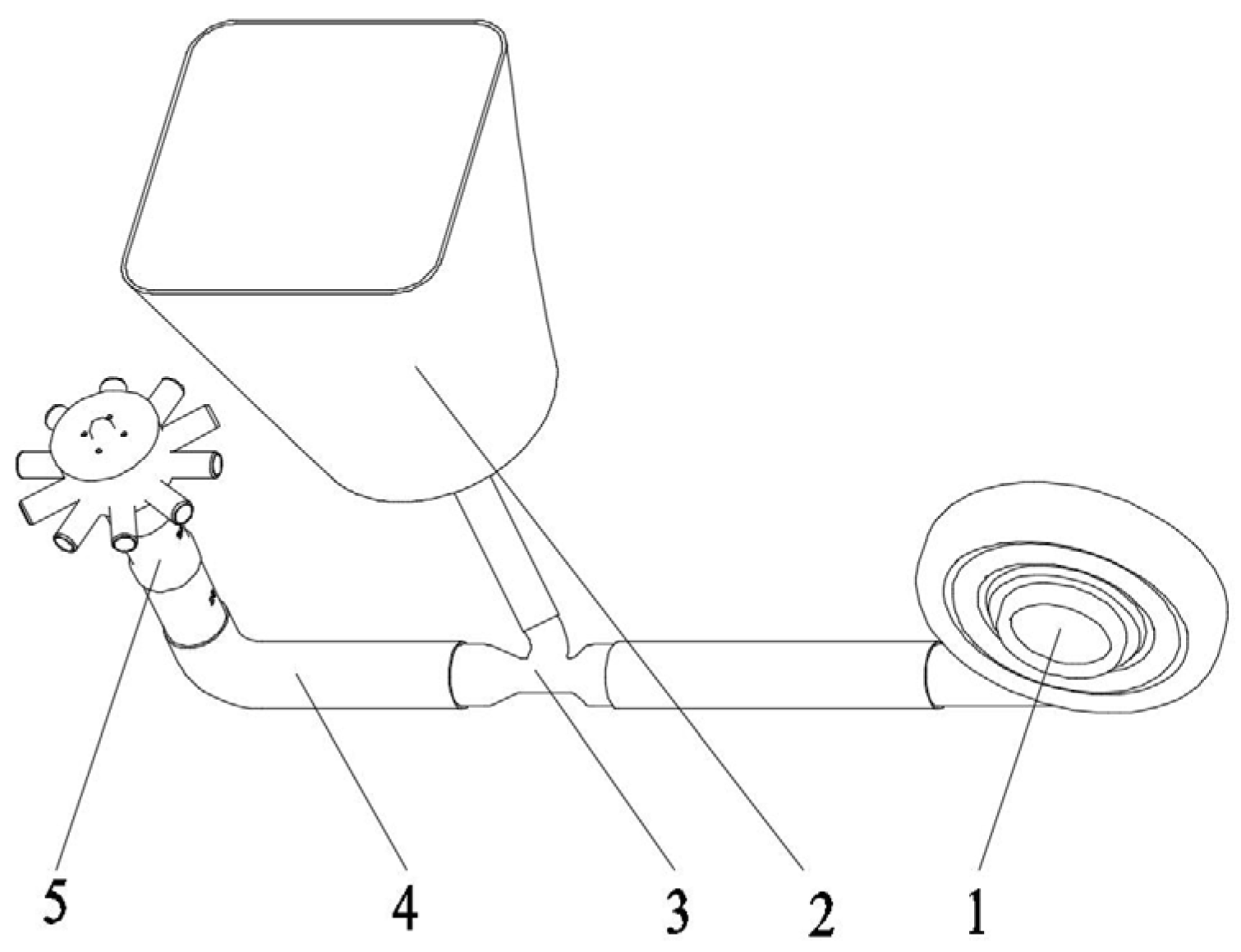
The structure of a pneumatic centralized fertilizer system is shown in Figure 1. Its working process can be divided into four stages: feeding, mixing, conveying, and distribution. During the fertilization operation, the motor controls the feeding device to discharge the fertilizer particles quantitatively. The fertilizer particles are mixed with the high-speed airflow generated by the fan with the action of gravity and the Venturi effect. The air–fertilizer mixed flow is transported to the elbow of the vertical distributor through the horizontal pipe. After passing through the elbow, the flow moves vertically to the top of the distributor and is then uniformly discharged at each outlet with the action of the distributor top cover, and finally enters the field through the conveying pipe.

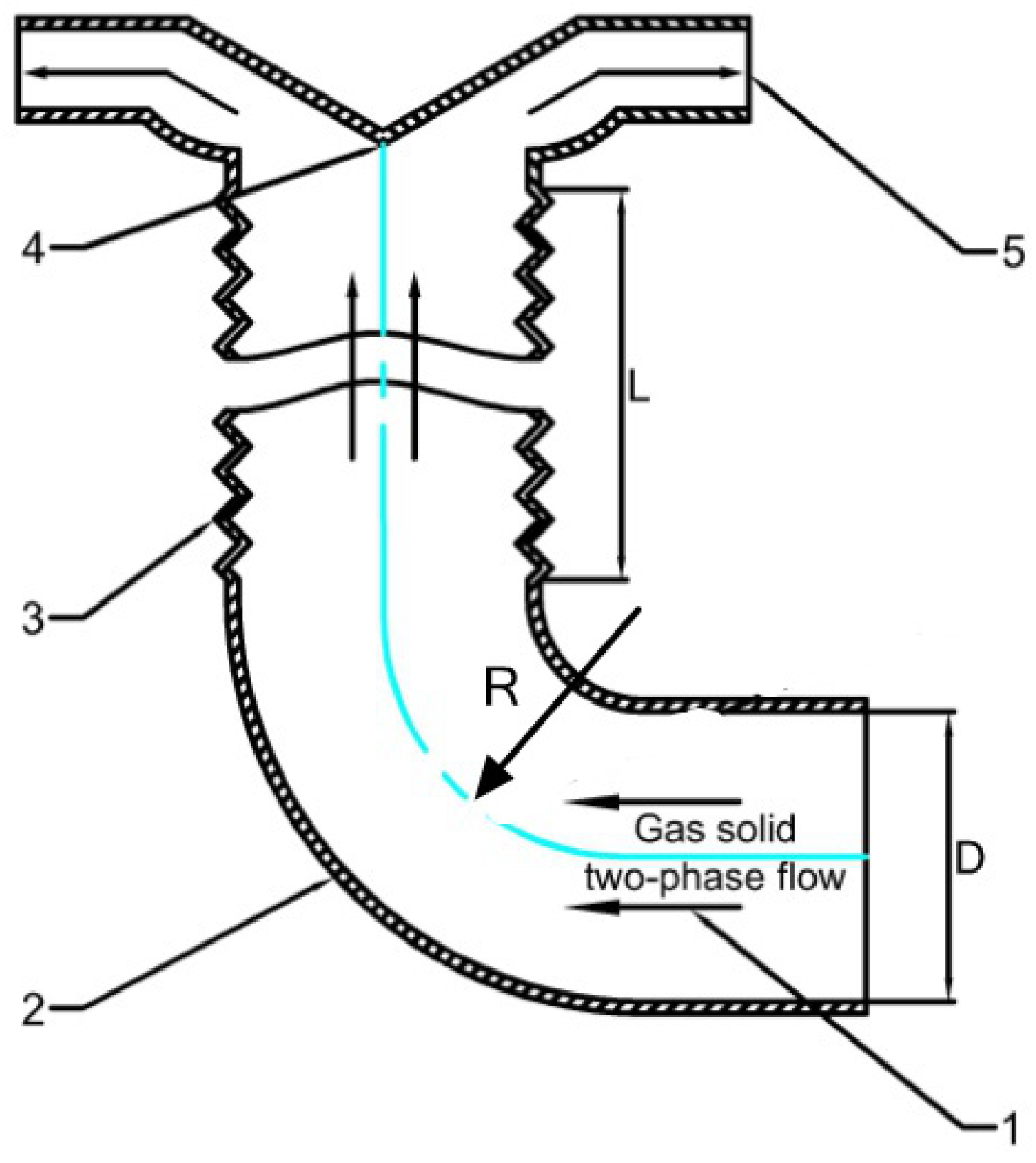
A vertical distributor is mainly composed of an inlet elbow, bellows, top cover, distributor shell, and outlet, as shown in Figure 2. The airflow carries fertilizer particles from the elbow into the vertical corrugated pipe. Because the fertilizer particles climb along the sidewall at the elbow, they are concentrated on one side when entering the corrugated pipe, resulting in an uneven distribution in the radial direction. However, the edge of the corrugated pipe has a significant resistance to the gas, and the air velocity at the center is relatively high; therefore, the particles tend to concentrate toward the center, and a relatively uniform gas–fertilizer mixed flow is gradually formed. Finally, the gas–fertilizer mixed flow is discharged from the outlet due to the collision with the top cover and the gas pressure difference.

In the whole process of fertilizer discharge, the inlet airflow velocity (v_g), particle feeding rate (M_s), corrugated pipe diameter (D), corrugated pipe length (L), and curvature diameter ratio of the elbow ($\varphi$) have an essential impact on the uniformity of the fertilizer discharge.

3. Materials and Methods

The structural and working parameters may include the inlet air velocity, particle–gas mass ratio, tube diameter, chemical fertilizer feeding rate, curvature diameter ratio R_b (elbow radius R/pipe diameter D), and corrugated pipe length, which will affect the trajectory and distribution uniformity of fertilizer particles. Therefore, their parameter range needs to be determined.

3.1. Basic Parameters of Fertilizer Distribution Systems

3.1.1. Inlet Airflow Velocity

The free suspension speed of fertilizer is a crucial aerodynamic characteristic. When the particles are suspended, buoyancy and gravity reach a balance. This can be expressed as follows:

$$C_D\frac{\pi }{4}{d}_p^2{\rho }_g\frac{v_p^2}{2}=\frac{\pi }{6}{d}_p^3\left({\rho }_p-{\rho }_g\right)g$$

(1)

The fertilizer particles are irregular spheres. By introducing the correction coefficient of irregularly shaped materials, the free suspension velocity can be written as

$$v_p=\frac{1}{\sqrt{k_s}}\times \sqrt{\frac{4}{3}\frac{d_p\left({\rho }_p-{\rho }_g\right)}{C_D{\rho }_g}g}$$

(2)

where C_D is the drag coefficient of the particles, d_p is the equivalent diameter of the particles (mm), ${\rho }_g$ is the air density (kg·m⁻³), ${\rho }_p$ is the particle density (kg·m⁻³), v_p is the free suspension velocity (m·s⁻¹) of a particle, g is the acceleration of gravity (m·s⁻²), and k_s is the correction coefficient of irregularly shaped materials. The drag coefficient is determined by the Reynolds number of particles, and the functional relationship is as follows:

$$C_D=\{\begin{array}{ll}\frac{24}{{\mathrm{Re}}_p}\left(1+0.15{\mathrm{Re}}_p^{0.687}\right)& {\mathrm{Re}}_p<1000\\ 0.44& {\mathrm{Re}}_p\ge 1000\end{array}$$

(3)

$${\mathrm{Re}}_p=\frac{{\rho }_g\left|v_g-v_p\right|d_p}{{\mu }_g}$$

(4)

where Re_p is the particle Reynolds number, μ_g is the gas viscosity (Pa·s), and ν_g is the air velocity (m s⁻¹). First, the value range of the particle Reynolds number was determined. The air density was 1.29 kg m⁻³, the particle diameter was in the range of 2–4 mm, the difference between the air velocity and the particle velocity was in the range of 5–30 m s⁻¹, and the gas viscosity was 1.82 × 10⁻⁵ Pa s. After substituting the above parameters into Equation (4), the particle Reynolds values were determined to be greater than 1000; therefore, according to Equation (3), the drag coefficient was 0.44. The particle density was 1641 kg m⁻³, and the correction factor for irregularly shaped materials was 1.2. After substituting the parameters into Equation (2), the free suspension speed of the particles was determined to be 9.7 m s⁻¹. Due to the complex pipeline structure of the fertilizer discharge device, the air velocity had to be at least 2.5 times the particle suspension velocity; that is, the air velocity was set at 25–35 m s⁻¹.

3.1.2. Fertilizer Feeding Rate

The feed rate of a fertilizer discharging device can be expressed as follows:

$$M_s=\frac{v_{s{l}_s{m}_s}}{3600}$$

(5)

where v_s is the machine’s forward speed (km h⁻¹), ls is the width of fertilization (m), and m_s is the total amount of fertilizer (kg hm⁻²). The fertilization rate for wheat, rice, and corn is generally 250–500 kg hm⁻², the maximum forward speed of the machine was 10 km h⁻¹, and the 10-row fertilization width was 2 m. The maximum fertilization mass per unit time of the fertilizer discharging device was calculated to be 270 g s⁻¹.

3.1.3. Corrugated Pipe Diameter

The volume of gas (V_g) passing through the pipe is related to the gas flow velocity and the pipe diameter, which can be expressed as

$$V_g=\frac{\pi D^2{v}_g}{4}=\frac{M_g}{{\rho }_g}$$

(6)

The particle–to–gas mass ratio (κ) can be used to quantify the relative amount of particles in the gas and can be written as

$$\kappa =\frac{M_{\mathrm{s}}}{M_g}$$

(7)

Combining Equations (6) and (7), the diameter of the fertilizer tube (D) can be written as

$$D=\sqrt{\frac{4M_s}{\pi \kappa v_g{\rho }_g}}$$

(8)

where M_g and ρ_g represent the air feed weight and the air density, respectively. As a result, M_s and ν_g were 270 g s⁻¹ and 25 m s⁻¹, respectively. ρ_g was 1.29 kg m⁻³, and the particle-gas mass ratio (κ) was 2, because the gas–solid flow was a diluted phase. According to Equation (8), the pipe diameter (D) could be calculated to be 70 mm.

3.2. Mathematical Model of Gas-Solid Two-Phase Flow

In the process of fertilizer discharge, the volume fraction of a solid in gas–solid two-phase flow is large. The particles are affected by airflow, and the collisions between particles and between particles and pipe walls. CFD–DEM is used to simulate the process of air conveying fertilizer particles. The fluid phase is solved based on the Navier–Stokes equations, while the particle movement is solved with Newton’s equations of motion. The fluid is regarded as a continuous incompressible fluid. The solution space is meshed, and the force of each particle is fed back to the Navier–Stokes equation by interpolation. In this approach, both particle–fluid and particle–particle interactions are taken into account.

3.2.1. Gas Phase Model

Considering the influence of turbulence and introducing the gas volume fraction (α), the governing equation of the standard k-ε turbulence model is as follows:

$$\frac{\partial \left(\alpha {\rho }_{\mathrm{g}}\right)}{\partial t}+\nabla \cdot (\alpha {\rho }_g{u}_g)=0$$

(9)

$$\frac{\partial \left(\alpha {\rho }_{\mathrm{g}}{u}_g\right)}{\partial t}+\nabla \cdot \left(\alpha {\rho }_g{u}_g{u}_g\right)=-\alpha \nabla p_g+\alpha {\rho }_{g}g+\nabla \cdot \left[\alpha \left(\mu +{\mu }_t\right)\left(\left(\nabla u_g\right)+{\left(\nabla u_g\right)}^T\right)\right]-S$$

(10)

where α represents the fluid volume fraction, ρ_g is the fluid density, and u_g and p_g are the fluid velocity and fluid pressure, respectively. g, μ, and μ_t are the gravitational acceleration, fluid viscosity, and turbulent viscosity, respectively. S is an interphase momentum exchange term that can be written as

$$S={\displaystyle \sum _{i=1}^N{F}_{g,i}/V_{cell}{}_{,j}}$$

(11)

where N is the particle number in cell j, while V_cell,j represents the volume of cell j, and F_g,i is the resultant force exerted on particle i.

3.2.2. Particle Dynamics

The two-phase flow of gas fertilizer particles can be regarded as a dilute phase gas–solid flow. The movement of each particle is governed by the gravity (F_GB), collision contact force (F_C), drag force (F_D), pressure gradient force (F_P), Saffman lift force, and Magnus force. The particle density ratio to the gas density is large (1000–2500); therefore, the gravity, drag force, contact force, and pressure gradient force are mainly considered. The translation and rotation of each particle can be expressed as follows:

$$m_p\frac{\mathrm{d}{u}_p}{dt}=F_{GB}+F_C+F_D+F_P$$

(12)

$$I_p\frac{d{\mathsf{\omega }}_p}{dt}={\displaystyle \sum }_{i=1,i\ne j}^{N_i}\left(\lambda \mathbf{n}\times {\mathbf{F}}_{ij}^t\right)$$

(13)

where m_p, u_p, and ω_p are the particle mass, particle translational velocity, and particle angular velocity, respectively. I_p is the moment of inertia, with a value of $\frac{2}{5}{m}_p{d}_p^2$d_p is the particle radius, λ represents the distance from the particle centroid to the contact point, n represents the unit vector, ${\mathbf{F}}_{ij}^t$ is the tangential contact force of particles i and j, and N_i is the number of all particles in contact with particle i. The gravity of the particles in the airflow can be expressed as follows:

$$F_{GB}={\mathrm{m}}_{\mathrm{p}}\left(1-\frac{{\rho }_g}{{\rho }_p}\right)g$$

(14)

The contact force of the particles can be divided into the tangential contact force and the normal contact force, and this division can be written as follows:

$$F_C={\displaystyle {\sum }_{i=1,i\ne j}^N\left(F_{ij}^n+F_{ij}^t\right)}$$

(15)

As shown in Figure 3, the normal and tangential contact forces of particles i and j can be expressed as follows:

$$F_{ij}^n=-\left(k_n{\ell }_n+{\eta }_n{\ell }_n^{\prime }\right)n_i{}_j$$

(16)

$$F_{ij}^t=\min \{\begin{array}{l}-\left(k_t{\ell }_t+{\eta }_t{\ell }_t^{\prime }\right)t_{ij}\hfill \\ -{\mu }_{\mathrm{ij}}\left|F_{ij}^n\right|t_{ij}\hfill \end{array}$$

(17)

where k_n and k_t are elastic coefficients, η_n and η_t represent damping coefficients, and ℓ_n and ℓ_t represent the normal and tangential overlapping displacements, respectively. μ_ij is the sliding friction coefficient between particle i and particle j, and t_ij is the unit tangent vector. In this CFD–DEM method, the Hertz–Mindlin model is used, and the elastic coefficients (tangential and normal) can be calculated as follows:

$${\mathrm{k}}_{n,ij}=\frac{4}{3}\frac{Y_i{Y}_j\sqrt{R_{ij}{\ell }_{n,ij}}}{Y_i\left(1-{\sigma }_i^2\right)+Y_j\left(1-{\sigma }_j^2\right)}$$

(18)

$${\mathrm{k}}_{t,ij}=\frac{16}{3}\frac{{\tau }_i{\tau }_j\sqrt{R_{ij}{\ell }_{n,ij}}}{{\tau }_i\left(2-{\sigma }_i\right)+{\tau }_j\left(1-{\sigma }_j\right)}$$

(19)

$$R_{ij}=\frac{R_i{R}_j}{R_i+R_j}$$

(20)

$${\tau }_i=\frac{Y_i}{2\left(1+{\sigma }_i\right)}$$

(21)

where Y_i and Y_j are the Young’s moduli of fertilizer particles i and j, respectively. R_ij is the equivalent radius of the particles. R_i and R_j are the radii of particles i and j, respectively. σ_i and σ_j are the Poisson’s ratios of particles i and j, respectively. τ_i and τ_j (the formula is similar to that for τ_i and is therefore not repeated) are the shear moduli of particles i and j, respectively. The collision of particles will cause energy dissipation. The transformation of pure kinetic energy into elastic potential energy cannot express the energy loss. It is necessary to introduce a damping coefficient to simulate the energy loss:

$${\eta }_{n,ij}=\sqrt{2k_{n,ij}{m}_{ij}}\frac{\left|\ln e_{n,ij}\right|}{\sqrt{{\pi }^2+{\ln }^2}{e}_{n,ij}}$$

(22)

$${\eta }_{\mathrm{t},ij}=\sqrt{2k_{t,ij}{m}_{ij}}\frac{\left|\ln e_{t,ij}\right|}{\sqrt{{\pi }^2+{\ln }^2{e}_{t,ij}}}$$

(23)

$${\mathrm{m}}_{ij}=\frac{m_i{m}_{{}_j}}{m_i+m_j}$$

(24)

where m_ij represents the effective particle mass, and m_i and m_j are the masses of particles i and j, respectively. e_n,ij and e_t,ij denote the normal and tangential recovery coefficients, respectively.

The drag force plays a major role in the momentum exchange between the fluid phase and the fertilizer particles. Additionally, the drag force depends on the relative velocity between the fluid phase and particles and is given by

$${\mathbf{F}}_D=\frac{V_p\beta }{1–\alpha }\left({\mathbf{u}}_g-{\mathbf{u}}_p\right)$$

(25)

where V_p is the particle volume. In addition to the relative velocity, the momentum exchange coefficient (β) between phases is another important parameter for the drag force calculation. The Gidaspow drag model was used in this study [25]. The interphase momentum exchange coefficient can be written as

$${\beta }_{Gidaspow}=\{\begin{array}{cc}\frac{150{\left(1-\alpha \right)}^2{\mu }_g}{\alpha d_p^2}+1.75\frac{\left(1-\alpha \right){\rho }_g\left|{\mathbf{u}}_g-{\mathbf{u}}_p\right|}{d_p}& \alpha \le 0.8\\ 0.75\frac{\alpha \left(1-\alpha \right){\rho }_g\left|{\mathbf{u}}_g-{\mathbf{u}}_p\right|}{d_p}{C}_D{\alpha }^{-2.65}& \alpha >0.8\end{array}$$

(26)

The pressure gradient force (F_P) received by the particle is related to the particle volume (V_p) and the fluid pressure gradient (∇P_g) as follows:

$$F_p=-V_p\nabla P_g$$

(27)

4. Results and Discussion

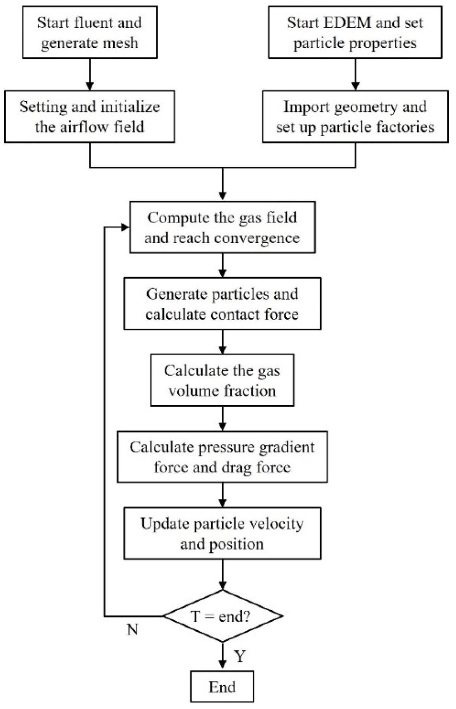
In the gas–solid coupling simulation, ANSYS Fluent and EDEM software were used to calculate the gas field and solid particles, and the momentum exchange between the gas and the solid was achieved with the user-defined function (UDF) coupling interface. The specific process is shown in Figure 4. The geometric model of the distributor was imported into Fluent and meshed. The inlet, outlets, and walls were defined for the model, and the air velocity was set at the inlet. 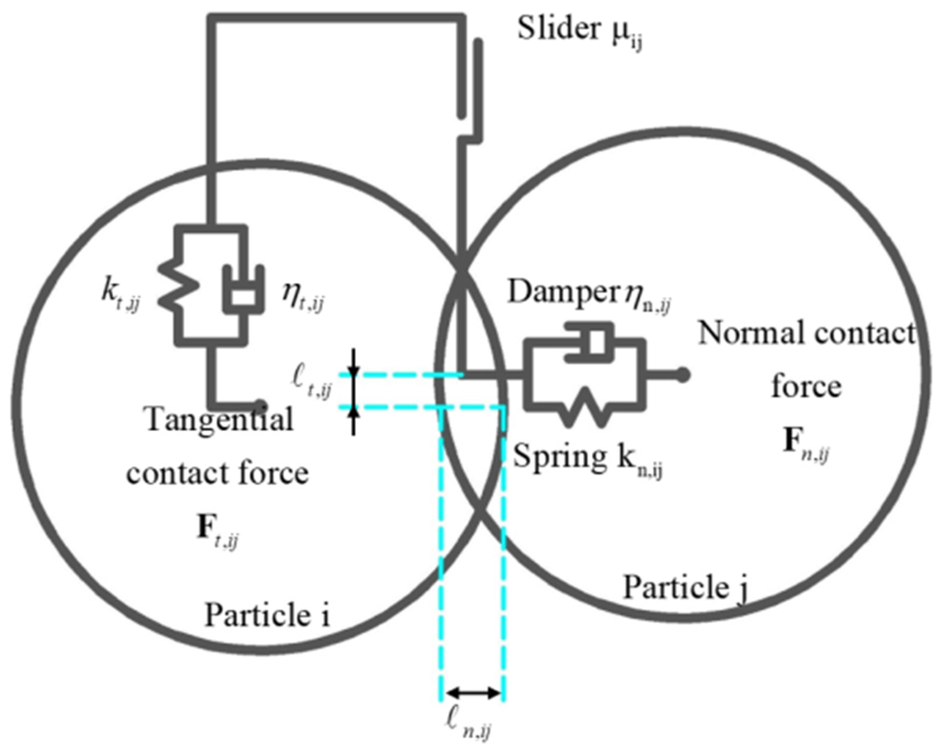The k-ε standard turbulence model was selected as the turbulence model, and the time step was 1 × 10⁻⁴ s, with 20 iterations per step. In EDEM, the distributor inlet and outlet attributes were named and set, a particle factory was set at the inlet to generate fertilizer particles at a speed of 270 g/s, and the weight of fertilizer particles passing through each outlet was counted using a user-defined program. The fertilizer particles were set as spheres with a diameter that was randomly distributed between 2 and 4 mm, and the Hertz–Mindlin contact model was used as the particle collision model. The UDF program was used to connect the Fluent and EDEM software, and the Gidaspow drag model was added to Fluent. At the beginning of the simulation, Fluent generated the flow field environment first, and then EDEM generated particles for coupling after 0.1 s.

Table 1. Computational parameters used in the simulations.

Materials	Parameter	Value
Fertilizer particle	Diameter range (mm)	2–4
	Density (kg/m3)	1641
	Poisson’s ratio	0.25
	Shear modulus (Pa)	1 × 107
Acrylic	Density (kg/m3)	1160
	Poisson’s ratio	0.41
	Shear modulus (Pa)	2.18 × 109
Particle to particle	Coefficient of restitution	0.3
	Coefficient of static friction	0.6
	Coefficient of rolling friction	0.3
Particle to acrylic	Coefficient of restitution	0.5
	Coefficient of static friction	0.6
	Coefficient of rolling friction	0.15
	Solid time step (s)	1 × 10−5
Gas phase	Gravitational acceleration (m/s2)	9.81
	Density (kg/m3)	1.29
	Viscosity (Pa·s)	1.81 × 10−5
	Fluid time step (s)	1 × 10−4

shows the specific properties and parameters of the particles and airflow [26].

4.1. Simulation Design

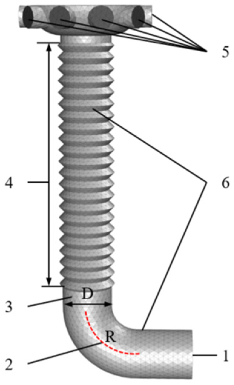
The experiment mainly tested the influence of different structural parameters of the distributor on the variation coefficient of the fertilizer discharge at each outlet. The main elements of the simulation model are shown in Figure 5. The length of the corrugated pipe (L), the R/D ratio, and the inlet air velocity (V_g) were taken as the test factors. Single-factor experiments with different parameters were used to study the effect of a single factor on the fertilizer performance for different levels. The single–factor experiment parameter settings are shown in

Table 2. Single-factor test parameters.

R/D Ratio	Fertilization Rate (g/s)	Length of Vertical Pipe (mm)	Air Velocity (m/s)
0.5	270	500	30
1
1.5
2
Air Velocity (m/s)	Fertilization Rate (g/s)	Length of Vertical Pipe (mm)	R/D Ratio
25	270	500	1
30
35
40

. The quadratic general rotary unitized design was used to study the effect of distributors with different parameter combinations on the fertilizer discharge uniformity. The parameter changes are shown in

Table 3. Simulation parameters of different distributors.

Number	Code Value	R/D Ratio	L (mm)	Vg (m/s)
1	1.682	0.5	300	25
2	1	0.7	340	27
3	0	1	400	30
4	−1	1.3	460	33
5	−1.682	1.5	500	35

.

The post-processing module of the EDEM software obtained the movement tracks and forces of the fertilizer particles. The user-defined function was loaded into the application programming interface to count the fertilizer weight flowing out of each outlet. To estimate the distribution accuracy, the coefficient of variation (CV) was used in this article.

4.2. Single Factor Test Results

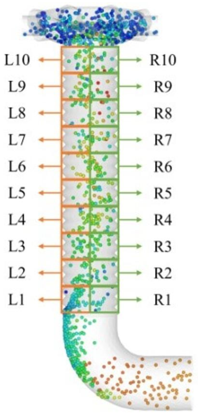
To test the influence of the length and the type of vertical pipeline on the particle distribution in the pipeline, as shown in Figure 6, the pipeline was divided into two types: a smooth pipeline and a corrugated pipe. Ten areas were divided on the left (L1–L10) and right (R1–R10) sides of the pipeline, and the weight of the particles passing in 0.5–3 s in each area was counted. The L/R ratio was defined to evaluate the uniformity of the particle distribution on the left and right sides of the pipe. The L/R ratio can be expressed as follows:

$$L/R=\frac{M_{Li}}{M_{Ri}}(i=1,\mathrm{2...10})$$

(28)

where M_Li represents the mass of particles passing through the Li area on the left, and M_Ri represents the mass of particles passing through the Ri area on the left.

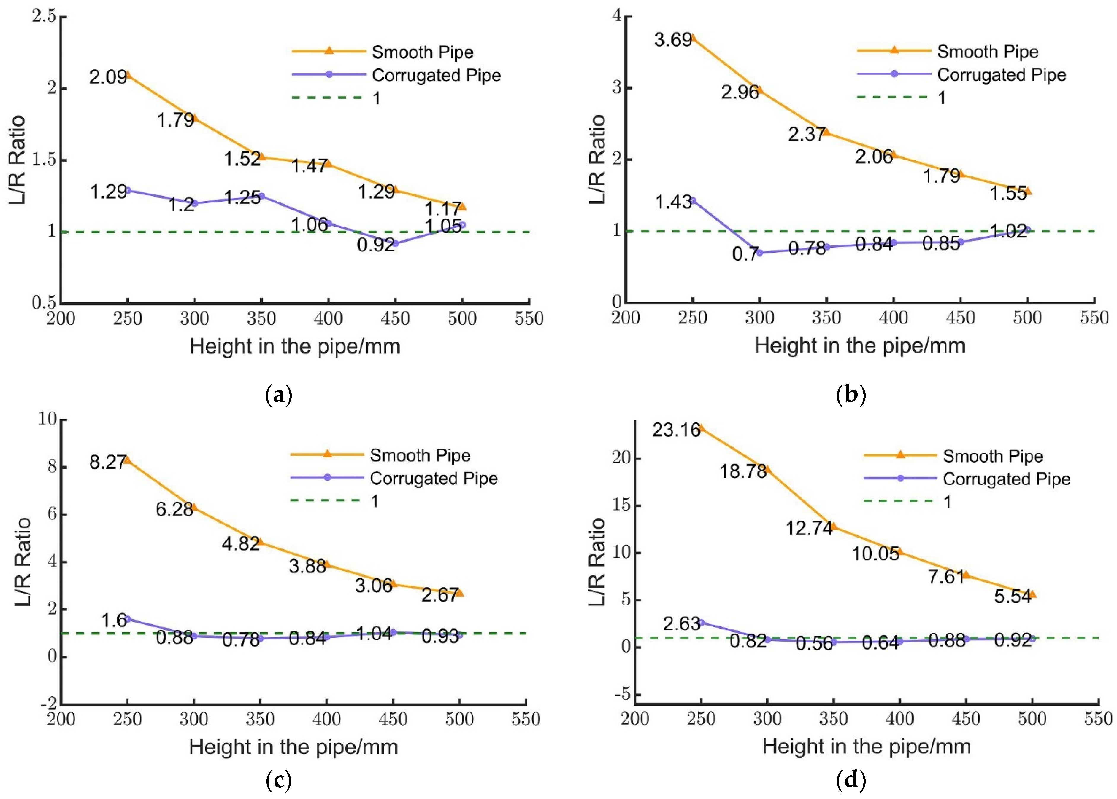
As shown in Figure 7, as the height of the corrugated tube and the smooth tube increased, the mass ratio of the particles distributed on both sides of the tube gradually tended toward 1. However, compared with the smooth tube, the corrugated tube could converge L/R to around 1 in a shorter length. It could be seen that the corrugated tube had certain advantages in uniformly distributing particles on both sides of the tube.

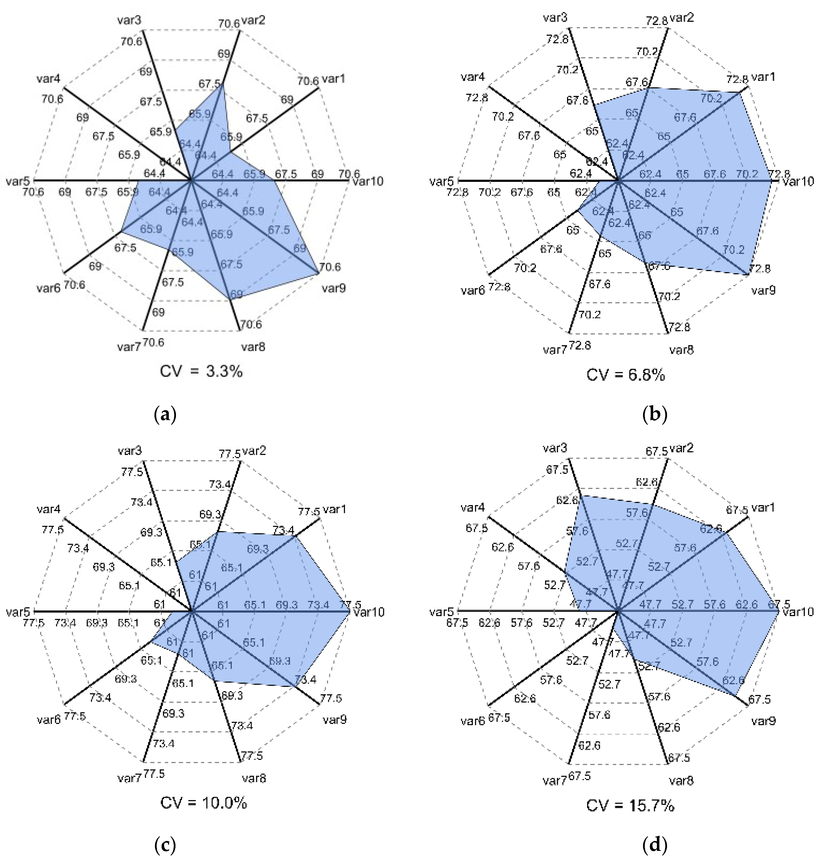
In the vertical smooth tube, as the value of R/D gradually increased, the L/R ratio increased significantly, indicating that a larger R/D value was not conducive to the uniform mixing of particles in the smooth vertical tube. In the vertical bellows, when the R/D value was in the range of 0.5–1, the L/R ratio could converge to around 1 at a vertical tube height of 400 mm. As shown in Figure 8, var10 is the exit facing the entrance direction of the elbow (corresponding to the right side of Figure 6). With the action of elbows with different R/D ratios, there were more particles distributed on the right half than on the left. When the R/D ratio was 2, this phenomenon was more obvious, leading to a significant increase in the CV. Therefore, the appropriate R/D ratio value was between 0.5 and 1.5.

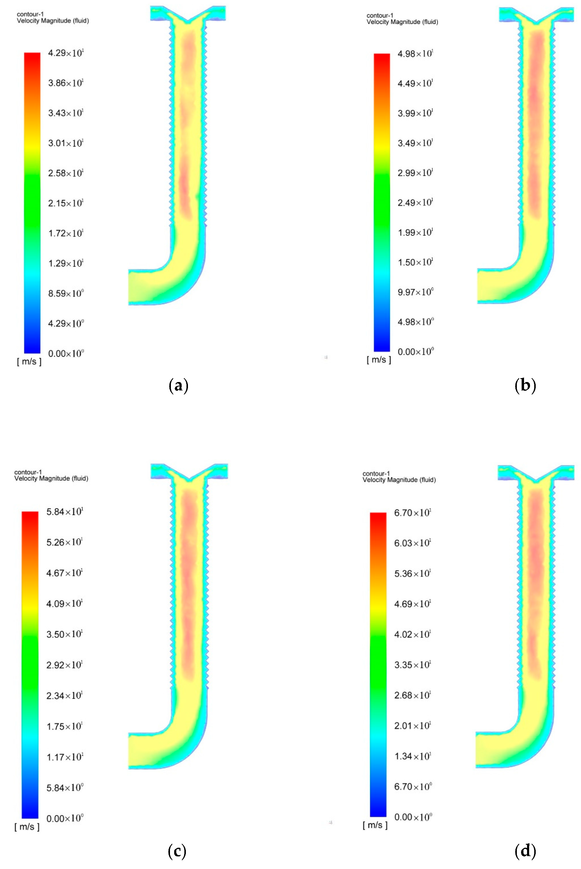
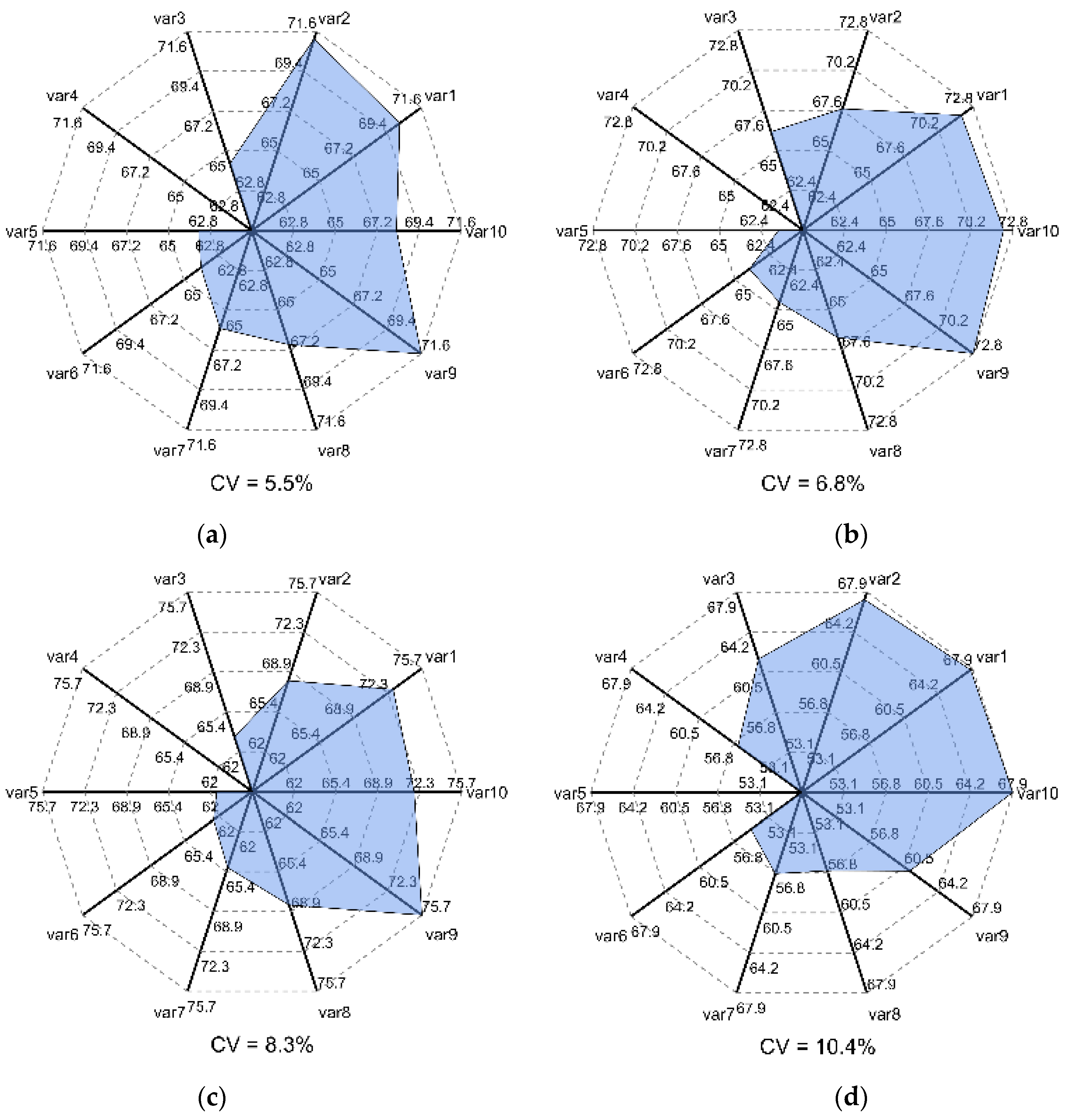
As the inlet air velocity increased, the peak air velocity at the center of the corrugated pipe increased from 43 m/s to 67 m/s, and the airflow energy was significantly improved. The excessive air velocity could not only easily cause particle breakage but could also increase unnecessary energy consumption. Therefore, the air velocity could not be too high. Figure 9 shows the coefficient of variation for the consistency of the displacement of each row corresponding to the four airflow speeds. As shown in Figure 10, the airflow speed increased from 25 m/s to 40 m/s, the coefficient of variation increased from 5.5 to 10.4, and the uniformity gradually decreased. Therefore, the airflow speed was appropriate. The value range had to be 25–35 m/s.

4.3. Combination Test Results

Design–Expert software was used to perform a quadratic regression analysis of the test data. The test results are shown in

Table 4. Test scheme and response value results.

No.	X1	X2	X3	X1X2	X1X3	X2X3	X12	X22	X32	Y/%
1	0.7	390	27	273	18.9	10,530	0.49	152,100	729	5.57
2	1.3	390	27	507	35.1	10,530	1.69	152,100	729	12.57
3	0.7	510	27	357	18.9	13,770	0.49	260,100	729	3.39
4	1.3	510	27	663	35.1	13,770	1.69	260,100	729	4.81
5	0.7	390	33	273	23.1	12,870	0.49	152,100	1089	7.38
6	1.3	390	33	507	42.9	12,870	1.69	152,100	1089	15.15
7	0.7	510	33	357	23.1	16,830	0.49	260100	1089	4.59
8	1.3	510	33	663	42.9	16,830	1.69	260,100	1089	8.39
9	0.5	450	30	225	15	13,500	0.25	202,500	900	3.28
10	1.5	450	30	675	45	13,500	2.25	202,500	900	9.99
11	1	350	30	350	30	10,500	1	122,500	900	10.65
12	1	550	30	550	30	16,500	1	302,500	900	3.83
13	1	450	25	450	25	11,250	1	202,500	625	5.5
14	1	450	35	450	35	15,750	1	202,500	1225	8.25
15	1	450	30	450	30	13,500	1	202,500	900	6.8
16	1	450	30	450	30	13,500	1	202,500	900	6.9
17	1	450	30	450	30	13,500	1	202,500	900	7.46
18	1	450	30	450	30	13,500	1	202,500	900	5.34
19	1	450	30	450	30	13500	1	202,500	900	6.95
20	1	450	30	450	30	13,500	1	202,500	900	5.91
21	1	450	30	450	30	13,500	1	202,500	900	5.76
22	1	450	30	450	30	13,500	1	202,500	900	6.3
23	1	450	30	450	30	13,500	1	202,500	900	5.6

, and the results of variance analysis are shown in

Table 5. Variance analysis of regression Equation.

Source	df	SQ	MQ	F	p-Value
Model	9	175.35	19.48	31.66	<0.0001 **
X1	1	71.69	71.69	116.49	<0.0001 **
X2	1	70.24	70.24	114.13	<0.0001 **
X3	1	13.95	13.95	22.67	0.0004 **
X1X2	1	11.40	11.40	18.52	0.0009 **
X1X3	1	1.24	1.24	2.02	0.1792
X2X3	1	0.02	0.02	0.03	0.8632
X12	1	1.14	1.14	1.85	0.1969
X22	1	3.69	3.69	6.00	0.0292 *
X32	1	1.97	1.97	3.20	0.0967
Residual	13	8.00	0.62
Lack of fit	5	4.02		1.52	0.2840
Pure error	8	4.22
Total	22	183.35

* Indicates significant difference, ** indicates extremely significant difference.

. The R/D ratio, bellow length, and airflow velocity had extremely significant effects on the coefficient of variation of the displacement consistency of each row. The order of the primary and secondary factors affecting the coefficient of variation of the displacement consistency of each row is as follows: the R/D ratio, bellow length, and airflow speed. There was a significant interaction between the length of the bellows and the bending diameter ratio of the elbow, and there was a certain interaction between the bending diameter ratio of the elbow and the airflow velocity. The -value of the lack of fit term of the regression model was not significant, and the regression equation was not lost. The regression equation of Y, which is the coefficient of variation in the distribution of fertilizers, is as follows:

$$Y=3.62+37.509X_1-0.0939X_2-0.3382X_3-0.06632X_1{X}_2+0.00014X_2^2$$

(29)

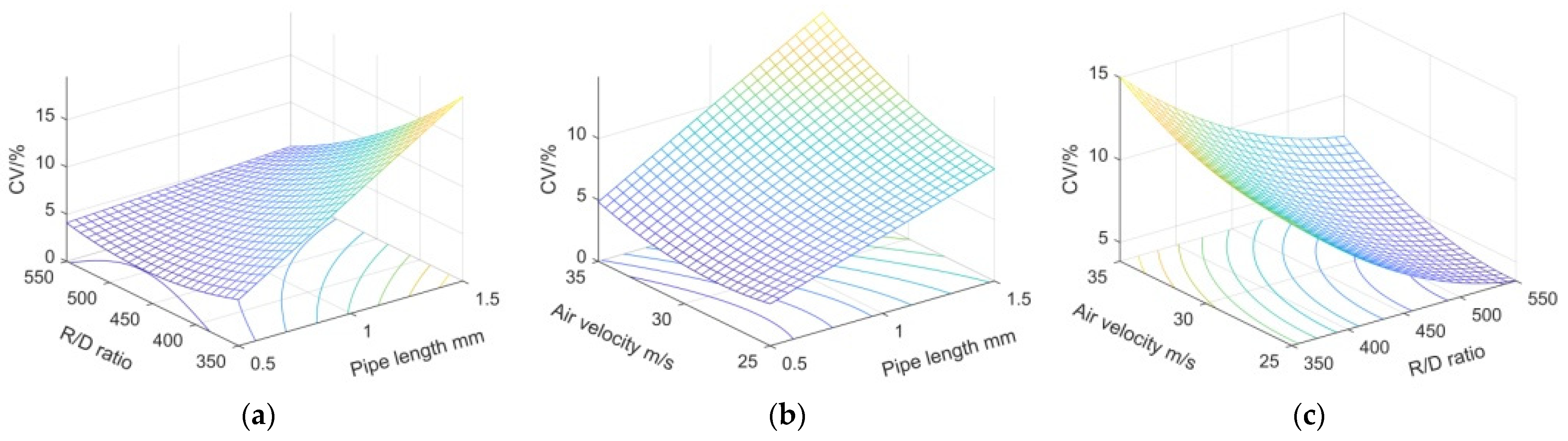
The interaction of the bending diameter ratio of the elbow and the length of the bellows on the coefficient of variation is shown in Figure 11a. When the airflow velocity was at the zero level, the length of the corrugated pipe was fixed, and the bending diameter ratio of the elbow was positively correlated with the coefficient of variation. The better range of the ratio was 0.5–0.7. When the bending diameter ratio of the elbow was constant, as the length of the bellows increased, the coefficient of variation first decreased and then increased. The preferred range of the length of the bellows was 400–500 mm.

The interaction of the bending diameter ratio and the airflow velocity of the elbow on the variation system is shown in Figure 11b. When the length of the bellows was at the zero level, the airflow velocity was fixed and the bending diameter ratio of the elbow was positively correlated with the coefficient of variation. The preferred range was 0.5–0.7. The bending diameter ratio of the elbow was in the range of 0.5–0.7, and the coefficient of variation had a minimum value. As the air velocity increased, the coefficient of variation first decreased and then increased. The optimal range of air velocity was 25–30 m/s.

The interaction of the air velocity and the length of the bellows on the coefficient of variation is shown in Figure 11c. When the bending diameter ratio of the elbow was at the zero level, the air velocity decreased, the length of the bellows increased, and the coefficient of variation decreased. The minimum value corresponded to the air velocity range from 25 m/s to 30 m/s, and the bellow length ranged from 500 mm to 550 mm.

4.4. Bench Test

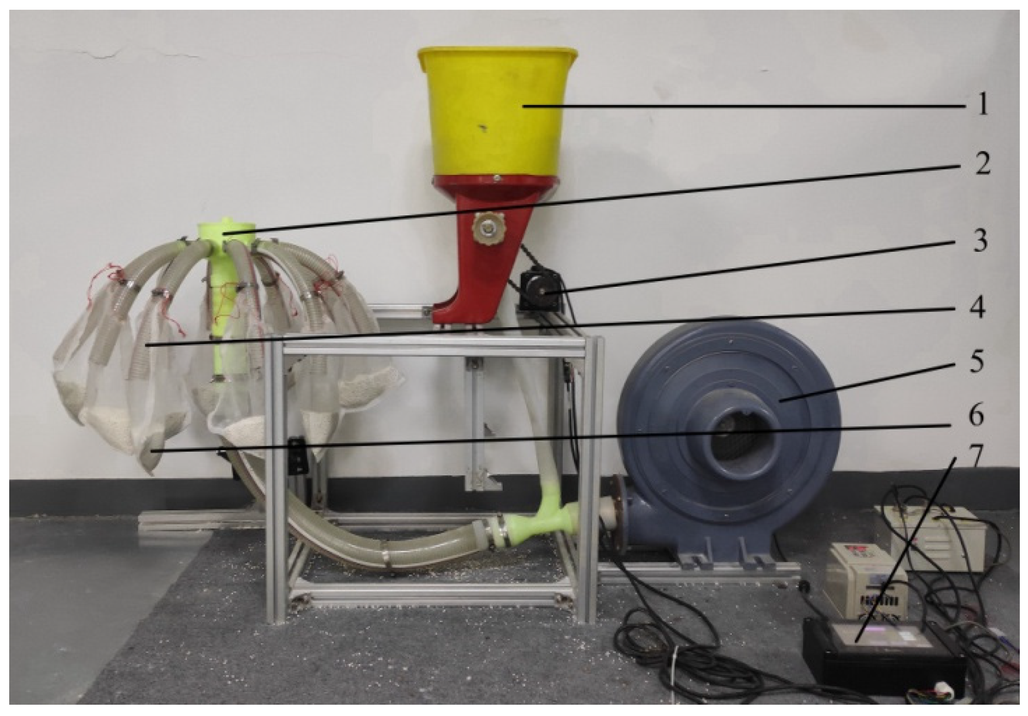
To verify the simulation results, a bench test was carried out using a pneumatic fertilizer discharging device test platform at the Intelligent Agricultural Machinery Laboratory of the Nanjing Institute of Agricultural Mechanization, Ministry of Agriculture and Rural Affairs. The study was conducted using a pneumatic centralized fertilizer discharge device (Figure 12). In the process of fertilizer discharge, the inlet air velocity was changed by controlling the fan speed, and the amount of fertilizer discharge was controlled by changing the speed of the fertilizer discharge groove wheel with the motor. There were yarn bags under each outlet pipe to collect the discharged fertilizer particles. Each experiment was conducted three times, and the fertilizer weight in the yarn bag was measured to obtain the average value.

The bench test data are shown in

Table 6. Results of validation experiments.

Air Velocity (m/s)	Fertilization Rate (kg/s)	Average Amount of Fertilizer (g)	CV (%)
25	0.07	72	3.7
	0.14	146	3.4
	0.21	208	4.9
	0.28	278	4.6
28	0.07	68	2.3
	0.14	142	3.1
	0.21	213	3.9
	0.28	283	4.3
31	0.07	74	4.2
	0.14	139	3.6
	0.21	204	4.8
	0.28	274	4.4

. The distributors with different test conditions, different fertilization rates, and different inlet wind speeds had a certain impact on the coefficient of variation of the discharge consistency of each row, but the overall coefficient of variation was not significant, and the coefficient of variation was much less than the 13% required in the technical specifications for the weight evaluation of fertilization machinery. The distributor could work normally under the conditions of different fertilization rates, the coefficient of variation did not exceed 5% under the conditions of small and large displacements, and the performance of the distributor was good. The test results showed that when the length of the bellows was 460 mm, the bending diameter ratio was 0.6, and the inlet air velocity was 28 m/s, the uniformity of the distributor was best, and the results were consistent with the simulation results.

5. Conclusions

Single-factor tests were carried out on the elbow diameter ratio, the length of the bellows, and the air velocity. The experiments showed that with the increase of the bending diameter ratio, the climbing phenomenon of the particles along the unilateral tube wall was more obvious, and it was easier to concentrate on one side, which was not conducive to the uniform mixing of particles and airflow. After the particles collided with the wall of the bellows and with the action of the radial and axial pressure difference of the airflow, they gradually mixed evenly with the airflow. The increase of the inlet air velocity caused the extreme value of the air velocity in the pipeline to increase significantly, which could easily cause particle breakage and was not conducive to reducing the coefficient of variation of the uniformity of the displacement of each row. It was determined that the value range of the bending diameter ratio of the elbow should be 0.5–1.5, the value of the bellow length should be in the range of 300–500 mm, and the inlet air velocity should be in the range of 25–35 m/s.

Through the quadratic orthogonal rotation combination experiment, the regression equation of the coefficient of variation of the displacement consistency of each row and each factor was obtained. After the analysis of variance, the importance of the factors affecting the coefficient of variation of the displacement consistency of each row was sorted as the elbow diameter, ratio, length of bellows, and air velocity. There was an interaction between the length of the bellows and the bending diameter ratio of the elbow, as well as between the airflow velocity and the bending diameter ratio of the elbow. The regression equation function was optimized and solved, and a variety of optimized parameter combinations were obtained, from which the optimal parameter combination was selected: the length of the bellows was 460 mm, the bending diameter ratio of the elbow was 0.6, and the inlet air velocity was 28 m/s. The bench test was performed on the optimal combination obtained by the simulation. The coefficient of variation of the distributor did not exceed 5% for the condition of increasing the displacement from a small displacement to a large displacement.