Stochastic Modeling of the Al Hoceima (Morocco) Aftershock Sequences of 1994, 2004 and 2016

Abstract

The three aftershock sequences that occurred in Al Hoceima, Morocco, in May 1994 (Mw 6.0), February 2004 (Mw 6.4) and January 2016 (Mw 6.3) were stochastically modeled to investigate their temporal and energetic behavior. A form of the restricted trigger model known as the restricted epidemic type aftershock sequence (RETAS) was used for the temporal analysis of the selected series. The best-determined fit models for each sequence differ based on the Akaike information criteria. The revealed discrepancies suggest that, although the activated fault systems are close (within 10 to 20 km), their stress regimes change and shift across each series. In addition, a stochastic model was presented to study the strain release following a specific strong earthquake. This model was constructed using a compound Poisson process and depicted the progression of the strain release during the aftershock sequence. The proposed model was then applied to the data. After the RETAS model was used to evaluate the behavior of the aftershock decay rate, the best-fit model was obtained and integrated into the strain-release stochastic analysis. By detecting the potential disparities between the observed data and model, the applied stochastic model of strain release allows for a more comprehensive examination. Furthermore, comparing the observed and expected cumulative energy release numbers revealed some variations at the start of all three sequences. This demonstrates that significant aftershock clusters occur more frequently shortly after the mainshock at the start of the sequence rather than if they are assumed to occur randomly.

1. Introduction

Seismic events can be classified into three main types based on their distribution over time [1]: (1) mainshock followed by a number of aftershocks decreasing in frequency, (2) slow build-up of seismicity leading to a type (1) sequence and (3) gradual increase and decay of seismicity without a distinct mainshock (seismic swarm), which occurs in areas with complex tectonic structures.

The decrease in aftershock occurrences caused by a strong earthquake can be studied using a wide range of methods, according to [2]. The Omori law model is the most typically adopted model [3], which [4] adapted into the modified Omori formula (MOF) by assuming that the fluctuation of the stress field of the mainshock initiates all the events in the sequence.

The trigger events are conditionally independent and follow a non-stationary stochastic Poisson process. Considering the complex behavior of some earthquake series, particularly in the presence of secondary events, [5] introduced the epidemic type aftershock sequence (ETAS) model, by increasing the capacity to generate secondary events for each event in the sequence. There are several triggering models between these two limit situations: the MOF and ETAS models being two of them [6,7]. The RETAS model [8] was developed by applying the principle of Bath’s law [9,10] to the subsequences caused by principal events, such as the mainshock. It is worth mentioning that the magnitude difference between the mainshock and the strongest aftershock is commonly considered to be constant, ranging between 1.2 and 1.4 on average, depending on the criterion [11], although with a lot of variability between individual aftershock sequences [12].

In this study, we focus on three sequences of type (1) designated as the aftershock sequences of Al Hoceima 1994, 2004 and 2016, occurring near the city of Al Hoceima, in Morocco (Figure 1 and Figure 2). The multifractal properties of these sequences have already been investigated in the framework of the spatial modeling of many seismic series in the Ibero–Maghrebian region [13]; however, even more temporal, energy and stress evaluations are required. Therefore, this study aims to examine three aftershock series using stochastic modeling.

This contribution includes the first section, which describes the regional geological context. In the second section, as suggested by [14], the three aftershock sequences are analyzed, and the stress regime in each series is comprehensively described. The Gutenberg–Richter relationship analysis, performed in a later section, attempts to derive reliable threshold magnitude values and b-value estimates for each sequence. A stochastic point process modeling analysis was performed in the previous two sections. As described previously, the aftershock decay rate was comprehensively studied using the RETAS model. The identified best-fit model was then integrated into a stochastic analysis of strain release. A comparison between the real values of the cumulative energy release and the expected modeled values is also examined and addressed.

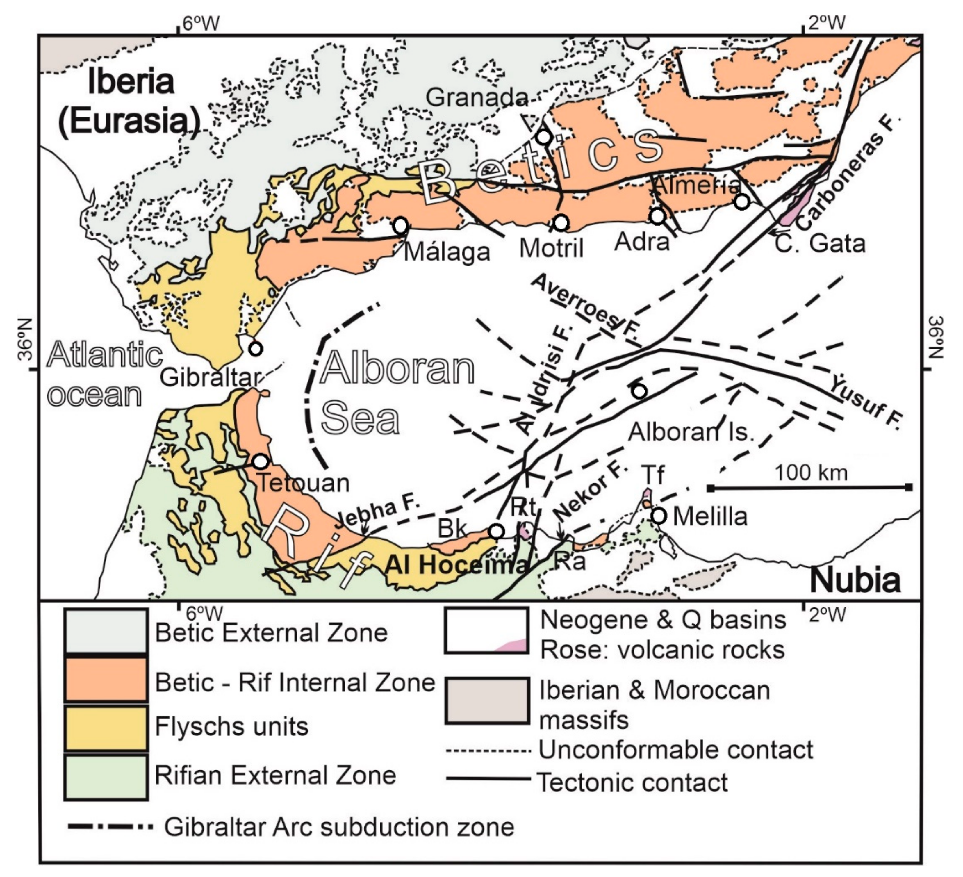
2. Geological Setting Overview

The Rif, along with the Betics, forms the westernmost alpine ranges of the Mediterranean Sea and are linked by the Gibraltar Arc. The Alboran Sea is in the center (Figure 1 and Figure 2). The central-south region of the Alboran Sea and the eastern Rif Cordillera belong to the seismically active area of Al Hoceima. The Internal and External Zones separated by the Flysch Units tectonically constitute the Rif Cordillera. In addition, several late intramontane Neogene–Quaternary sedimentary basins emerged, some of which were linked to the Alboran Sea, forming the largest basin of the orogen [15].

The Internal Zone comprises Sebtide and Ghomaride superposed tectonic complexes formed by Paleozoic, Mesozoic and Cenozoic rocks, which are strongly affected by the Alpine Orogeny and have their equivalents in the Betics, called Alpujarride and Malaguide. Some of these complexes have undergone metamorphism and have been thrust over the Flysch Units and the External Zone in the Rif.

The Flysch Units, which are mostly Tertiary sedimentary rocks with some locally ultrabasic rocks, constitute the sedimentary basin that separates the Internal and External Zones and is underlain by oceanic crust. They thrust southward across the External Zone, which is formed by Mesozoic and Cenozoic sedimentary rocks that are mostly unmetamorphosed or, in some cases, have a low degree of metamorphism.

The Alboran Sea is primarily formed by Neogene and Quaternary sediments deposited on a basement that corresponds to the Internal Zone complexes [16]. Furthermore, Neogene to Quaternary volcanic rocks can be found in the central-eastern Alboran Sea and eastern Rif and Betics.

The main alpine deformations in this area occurred throughout the Oligocene and Miocene and continue into the present. The earliest stages of deformation were partially simultaneous with the process of western migration of the Betic and Rif Internal Zones, coinciding with the opening of the Alboran Sea and forming the Gibraltar Arc during a period of severe weakening of the continental crust. The new Alboran marine area corresponds to the western end of the Algero–Provençal Basin, which began to open at the end of the Oligocene [17], forming a new oceanic floor. In the Alboran Sea, the continental crust was markedly weaker and situated on the new oceanic floor on its eastern border.

Subduction processes, combined with NNW–SSE convergence and regional compression of the Iberian and Nubian plates [18,19,20], resulted in significant deformation in the northern and southern borders of the earliest Alboran Sea. These processes developed the Gibraltar Arc, with the uplift of the Rif and Betic Cordillera, which were radially deformed [21] around the Alboran Sea and undergoing a regional E–W compression.

Later, from the late Miocene, when the opening was nearly at its end ceasing the E–W compression, the general NNW–SSE compression was completely re-established [22]. The region then began to undergo folding (e.g., the Alboran Ridge anticline) and faulting (e.g., the Al Idrisi, Yusuf, Carboneras, Averroes, Jebha and Nekor faults, in addition to other minor faults).

Since the Miocene, important NNE–SSW sinistral strike-slip fault systems crossing the Alboran Sea (Trans Alboran shear zone; [23]) were formed, such as the Carboneras Fault, coming from Almería, Spain and the Nekor and Jebha faults, the last being renowned inland [24]. Later, the Al Idrisi and other conjugated NW–SE faults developed (e.g., the Averroes Fault), as well as some E–W faults and thrusts with a general ENE–SWS strike. The upper Neogene and Quaternary sediments of the central and eastern Alboran Sea are affected by these deformations, whereas the western Alboran Sea undergoes mud volcanic tectonics [25]. This regional geodynamic setting continues into the present.

Almost all the domains mentioned are present in the study area. The Internal Zone forms the inland Bokoya Massif, between Al Hoceima and Melilla to the west, as well as a smaller outcrop, Ras Afrou, on the coast between Al Hoceima and Melilla. The Flysch Units and External Zones, as well as several Neogene–Quaternary basins, appear south of the Internal Zones. Furthermore, Miocene volcanic rocks comprise most of the Raf Tarf and Tres Forcas capes. There are also significant faults (Figure 1 and Figure 2), the most notable of which are located around the Nekor Basin limits, east of Al Hoceima, whose directions range from nearly N–S to NE–SW (e.g., the Trougout Fault, separating Ras Tarf volcanic rocks from Al Hoceima Bay). Some of these faults remain active offshore.

Evidently, all existing seismogenic faults, both onshore and offshore, are unknown, particularly because some are in the early stages of development [26].

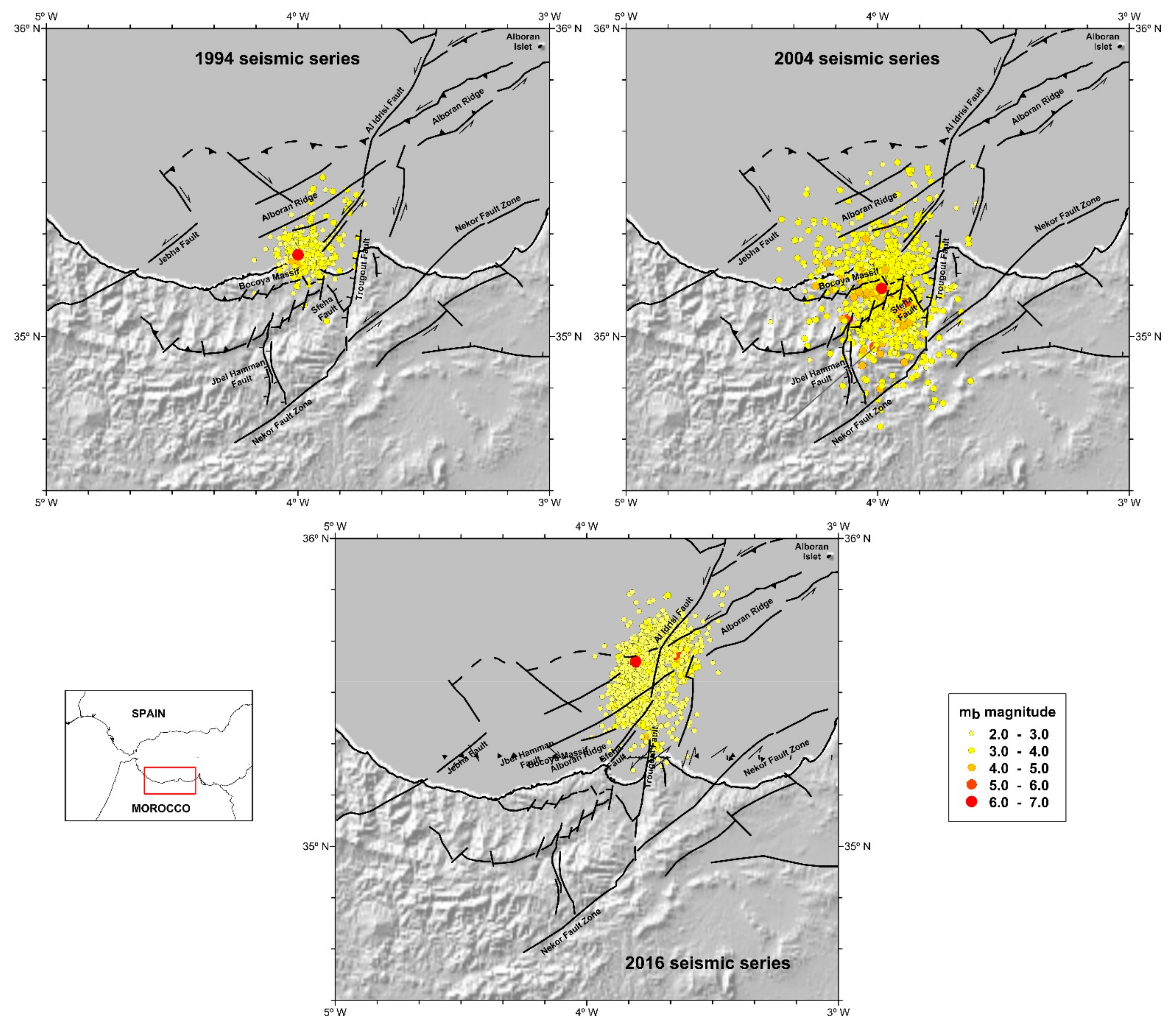
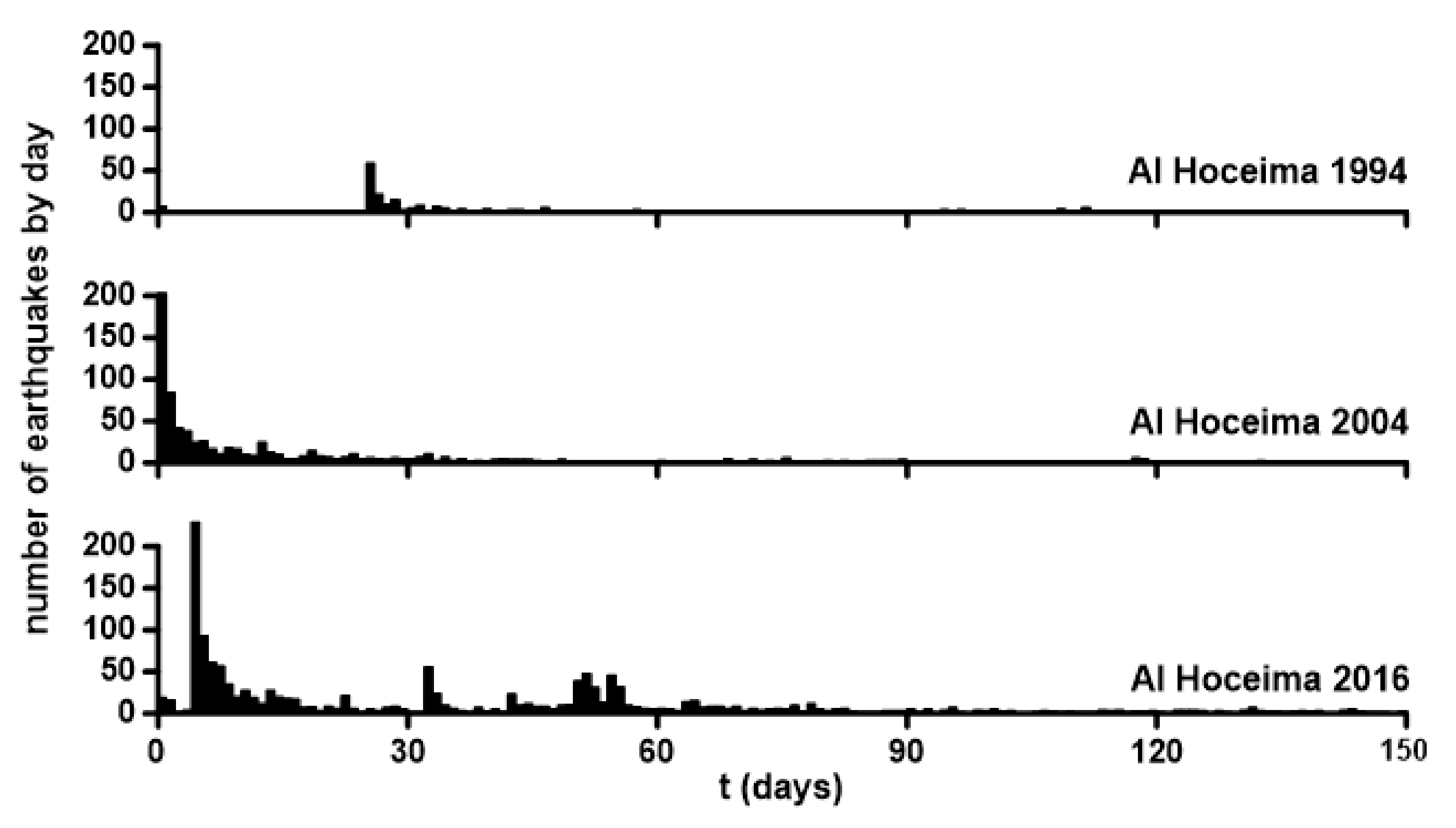
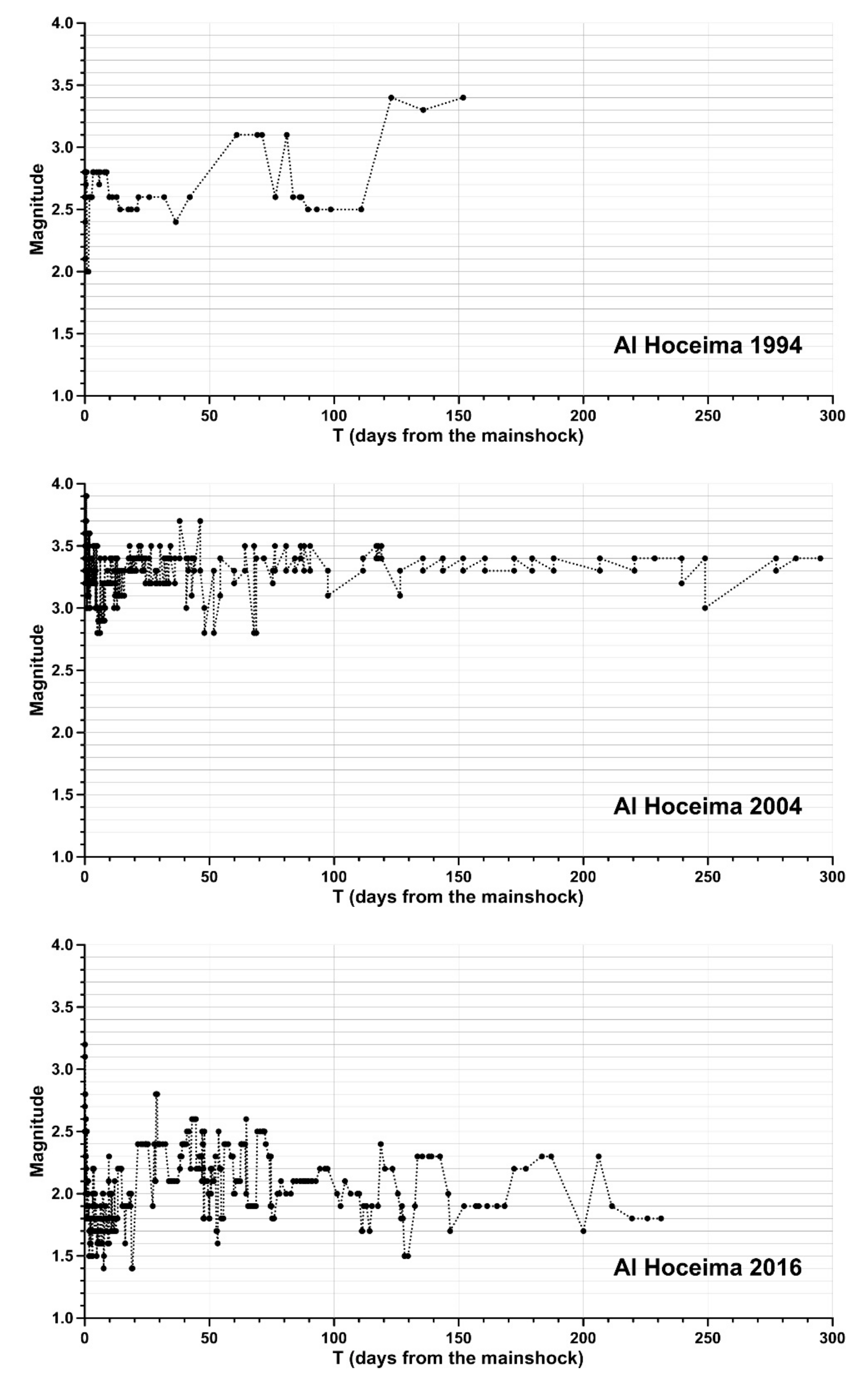
3. Aftershock Sequences Description

The Alboran region, specifically the Al Hoceima region, has been the subject of numerous tectonic studies, including those by [27,28,29,30,31]. Owing to its location in the complex border zone between the Eurasian and Nubian plates, near the border between the eastern Rif Cordillera tip and the Alboran Sea, the Al Hoceima region is known to be the most seismically active sector in northern Morocco. Furthermore, because of its strong seismicity, it is one of the most seismically active sites in the western Mediterranean region.

The seismic database of the Spanish Instituto Geográfico Nacional (IGN) was used to assemble the data for this study, with no further processing or parameters from other local or regional agencies. This was performed to keep the database as homogeneous as possible, working in all cases with m_b magnitude.

The 1994 earthquake sequence (Figure 2) began on 26 May 1994, with a strong earthquake of magnitude Mw 6.0, which struck the coastal region near Al Hoceima. This event had a strong impact on the studied region of Al Hoceima [32]. The maximum felt intensity was VIII–IX (EMS-98), indicating an extended NNE–SSW corridor that accounted for over 80% of the damage reported. The magnitude of the earthquake was revised to Md 5.7 (Moroccan Scientific Institute), and the epicenter was relocated north of Al Hoceima at a focal depth of 13 km. According to [32], the distribution of aftershock epicenters in Figure 2 is largely scattered along a NNE–SSW trending cluster over an almost vertical plane.

Another seismic series struck the region on 24 February 2004, with a damaging mainshock of Mw 6.4 (Figure 2). This event occurred on land and caused severe damage. Ref. [33] estimated the maximum perceptible intensity around XI (EMS-98). In Al Hoceima and the surrounding area, nearly 630 people died, 926 were injured, and nearly 15,000 were left homeless. Ref. [34] relocated the 2004 sequence. According to [35] and other authors, the series epicenter occurred on a NE–SW trending strike-slip fault, while the presence of a NW–SE fault with conjugate NE–SW branches cannot be ruled out [34].

The third examined sequence (Figure 2) is linked to the major event on 25 January 2016 (Mw 6.3), whereas it is possible that the series began on January 21 with an event of Mw 5.1. Following these events, a major earthquake series with decreasing activity occurred in 2016 and 2017 [33,35,36]. The major event, with a maximum intensity of VI–VII, was felt over the Alboran area, particularly in Melilla, Spain, on the northern African coast, where extensive damage was reported, as well as in Al Hoceima [33,37].

The Spanish IGN found two distinct epicenter clusters in 2016, each with distinct tendencies. The first one is aligned NNE–SSW changing to N–S, with dominant strike-slip focal mechanisms, while the second one is to the northeast of the first, with a rounded shape and a dominant reverse focal mechanism solution. A NNE–SSW subvertical fault, roughly parallel to the elongation of the alignment and displaced west of the Al Idrisi Fault, is linked to the main NNE–SSW alignment [26].

Figure 3 shows the number of events per day for the selected series in the 150 days after the mainshock, while

Table 1. Number of events (n), minimum recorded magnitude (M_min), computed threshold magnitude (m_c) using the Maxc method and a and b-parameters.

Sequence	n	Mmin	mc	a ± σ	b ± σ	Sequence
1994	263	2.0	2.8	5.05 ± 0.02	1.01 ± 0.07	1994
2004	969	1.5	3.4	6.56 ± 0.02	1.14 ± 0.05	2004
2016	2577	0.8	2.0	4.86 ± 0.03	0.82 ± 0.02	2016

provides the number of events in each series, the minimum recorded magnitude and other computed parameters, which will be discussed later. The 1994 Al Hoceima sequence had 263 recorded events with a magnitude above 2.0, which occurred until December 1994 (some early events have been included in the series); the 2004 sequence had 969 recorded events with a magnitude above 1.5, which occurred until February 2005; and the 2016 Al Hoceima sequence had 2577 recorded events with a magnitude above 0.8, which occurred until August 2016.

For the 1994 and 2004 sequences, Figure 3 reveals a direct decrease in the number of events per day over time, whereas the trend for the 2016 series is more complex, apparently because of the complexity of the rupture(s). There were several different phases in the late aftershock sequence. The recorded occurrences followed a deformation band with two unambiguous alignments with widths of less than 10 to 20 km for the first 30 days [26]. The main alignment, which is moved 5–10 km westward, appears to be spatially associated with the Al Idrisi Fault. A decrease in the seismic activity rate was observed over the next 30 days, resulting in an increase in the width of both alignments, which reached 10–20 km. A clear decrease in activity rate was observed at least 60 days after the mainshock, affecting a wider area than 15–25 km in width as [26] indicated.

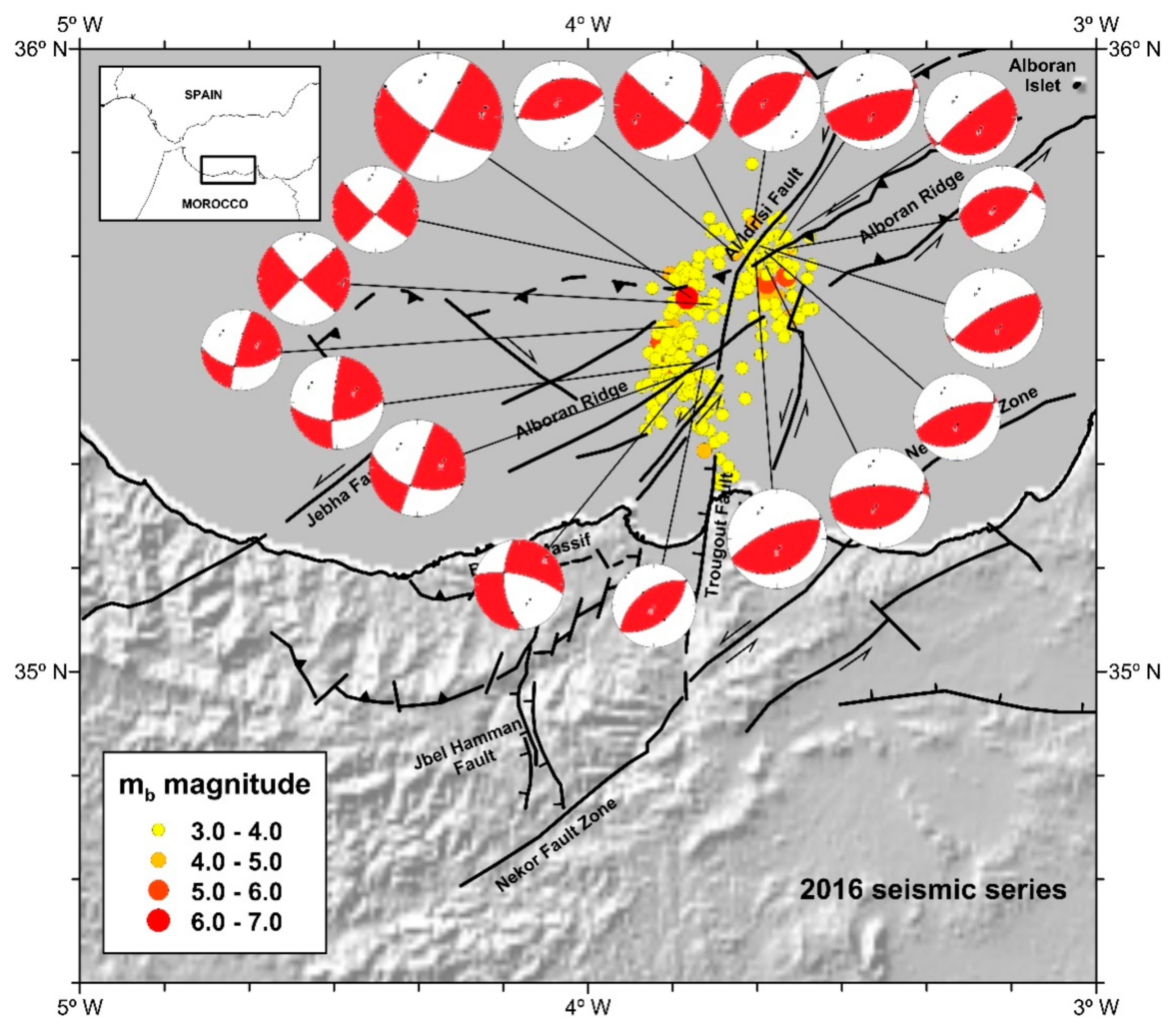
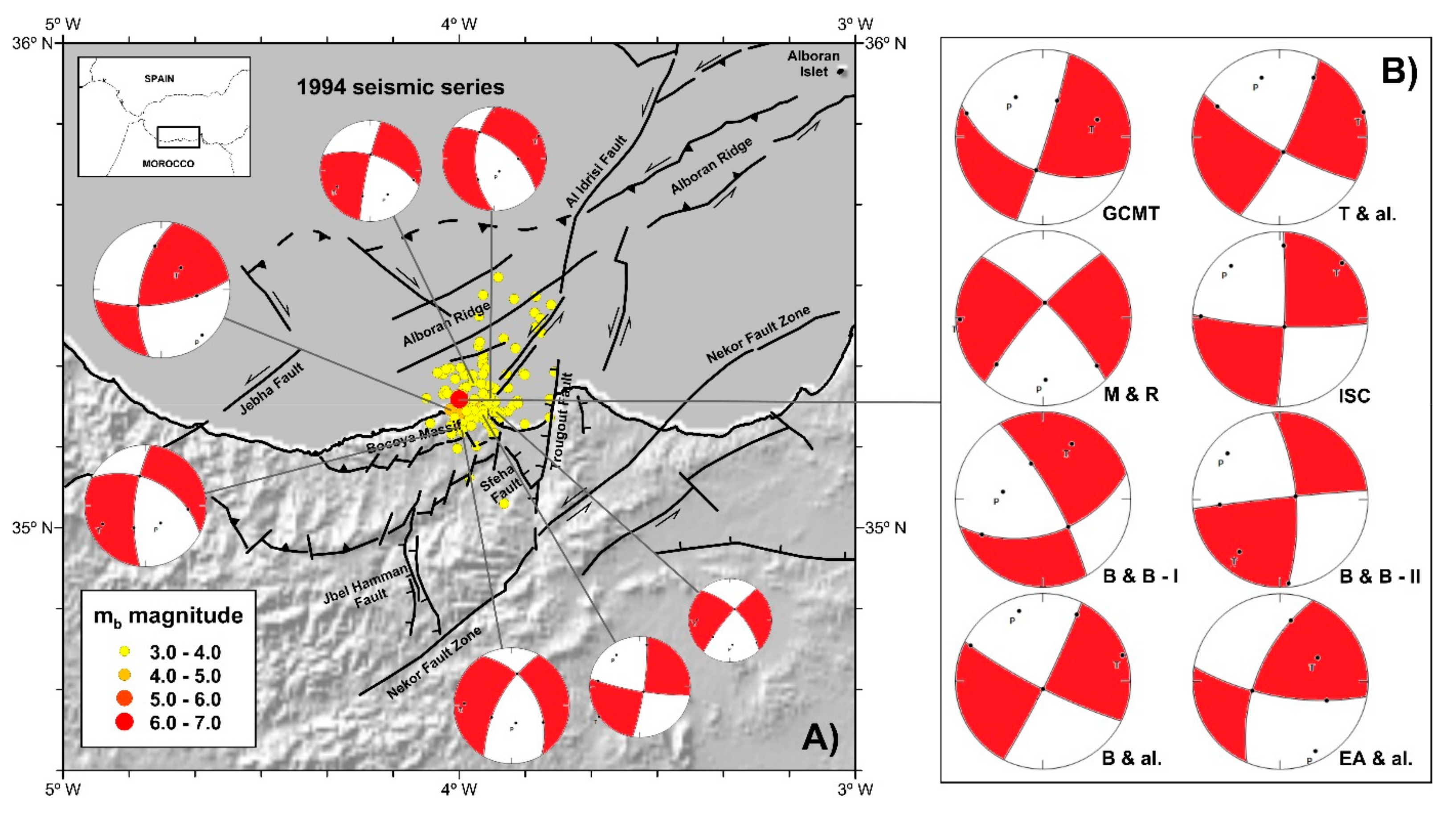
4. Seismic Series Stress Regime

The IGN database, international agencies and numerous studies aimed at analyzing these seismic series were used to obtain earthquake focal mechanisms for the selected series. Figure 4 shows earthquakes with magnitudes greater than 3.0, from the 1994 Al Hoceima sequence, as well as the focal mechanism of aftershock events computed by [32] (Figure 4A); different solutions for the focal mechanism of the main shock (Figure 4B) from the Global Centroid Moment Tensor (GCMT), International Seismological Centre (ISC); and specific works by [38,39,40,41] (for both a pre-event and the main quake) and [29].

Figure 5A depicts the distribution of events with magnitudes greater than 3.0, which were included in the 2004 series, as well as the estimated focal mechanisms of the largest events. In addition, Figure 5B shows the earthquakes and computed focal mechanisms of the so-called “eastern cluster” from [34].

Figure 6 shows events with magnitudes more than 3.0 as well as estimated focal mechanism solutions for the 2016 Al Hoceima sequence.

The stress pattern from the inversion of the available focal mechanism data was used to characterize the three seismic series. It is worth noting that for the inversion process, it was not necessary to select between two available nodal planes. To estimate the different parameters of the reduced stress tensor, we used the improved right dihedron method [42] combined with the iterative rotational dihedron method [43]. Our aim was to calculate the four parameters of the reduced stress tensor, σ₁, σ₂, σ₃ and the stress ratio, R = (σ₂ − σ₃)/(σ₁ − σ₃).

According to [19], this method allows for estimating previous parameters and the extraction of filtered focal mechanism data by deleting nodal planes that are incompatible with the average stress regime. The compatible focal mechanisms and the calculated stress tensor produced at this point were then employed as the direct starting point for the rotational optimization technique.

The iterative grid-search rotational optimization process is based on a controlled grid search of the stress tensor using the Win-TensorTM code to reduce the so-called misfit (F5) [44]. According to [45], the nodal plane best explained by the stress tensor was chosen as the actual fault plane from the two planes of the focal mechanism. Consequently, the final inversion examines the focal planes that a uniform stress field best fits [46]. After the ultimate optimization, the omitted focal planes must be reconsidered without modifying the stress tensor. If this is the case, the data are re-entered into the database, the stress tensor is re-optimized, and the software runs another check for the rejected data.

This method was used to analyze the focal mechanism data for each seismic sequence.

Table 2. Stress regime for the cases considered in Figure 7.

Sequence	σ1	σ2	σ3	R	F5
1994 main event	327° N/13°	226° N/40°	072° N/47°	0.19	7.1
1994 aftershocks	132° N/44°	349° N/39°	242° N/20°	0.38	3.5
2004 all, without ‘eastern’ cluster	330° N/25°	149° N/65°	239° N/00°	0.59	2.6
2004 ‘eastern’ cluster	020° N/79°	141° N/06°	232° N/09°	0.82	5.6
2016 main cluster	332° N/06°	224° N/72°	064° N/17°	0.74	1.6
2016 secondary cluster	330° N/23°	062° N/04°	161° N/67°	0.49	3.3

and Figure 7 show the results of the stress inversion. Several authors (e.g., [19,44,47,48,49]) have used a similar approach to investigate the stress regime in other regions.

The variability in the stresses is highlighted in Figure 7 and Table 2. The different solutions of the mainshock, when considered together, and those determined for the aftershocks were not very distinct in the 1994 seismic series. A prolate stress ellipsoid with a near NW–SE horizontal (compressive stress regime) and roughly similar σ₂ and σ₃ values appeared in the mainshock. The slope then turns southeast, highlighting the NE–SW expansion with the horizontal σ₃ being more noticeable (extensive stress regime).

The seismic series from 2004 appears to be more uniform, with oblate stress ellipsoids and a noticeable NE–SW extension trend. While the main cluster shows NW–SE sub-horizontal σ₁ and NE–SW sub-horizontal σ₃ values, clearly indicating a strike-slip stress regime, in the “eastern cluster” [34], a cluster with a few low-energy earthquakes and σ₁ and σ₂ values becoming closer, and a NE–SW horizontal extension is dominant (extensional stress regime).

In the 2016 sequence, the computed stress regime for the main cluster agrees with that obtained in the 2004 main cluster (strike-slip stress regime); however, there is a noticeable increase in the axial ratio, where σ₁ and σ₂ magnitudes are closer, highlighting the well-defined NE–SW sub horizontal extensive stresses. In contrast, the secondary cluster is dominated by NW–SE compressive σ₁ stresses and a subvertical σ₃, suggesting thrusting (compressional stress regime). Furthermore, the secondary cluster stresses are like those obtained for the mainshock of 1994, which had a primary NNW–SSE σ₁ odd axis.

The maximum compressive horizontal stress (SHmax) in all solutions was between 142° N and 153° N, which is consistent with previous results for regional stresses (e.g., [18,19,20,50]). However, the extension directions are compatible with the Internal Zone movement of the Betic–Rif toward the southwest [26,51,52,53].

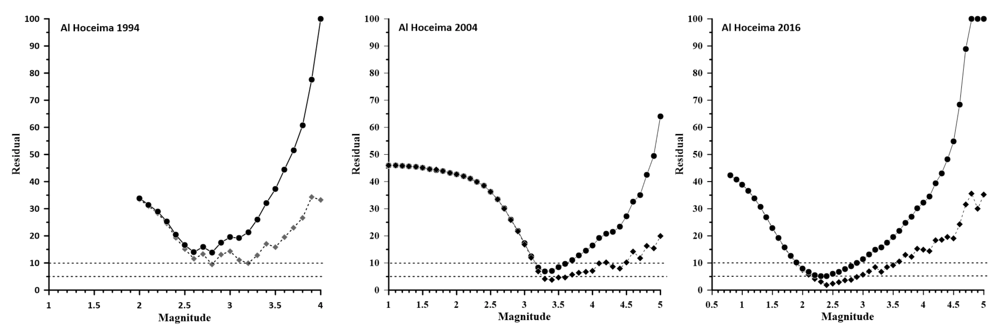
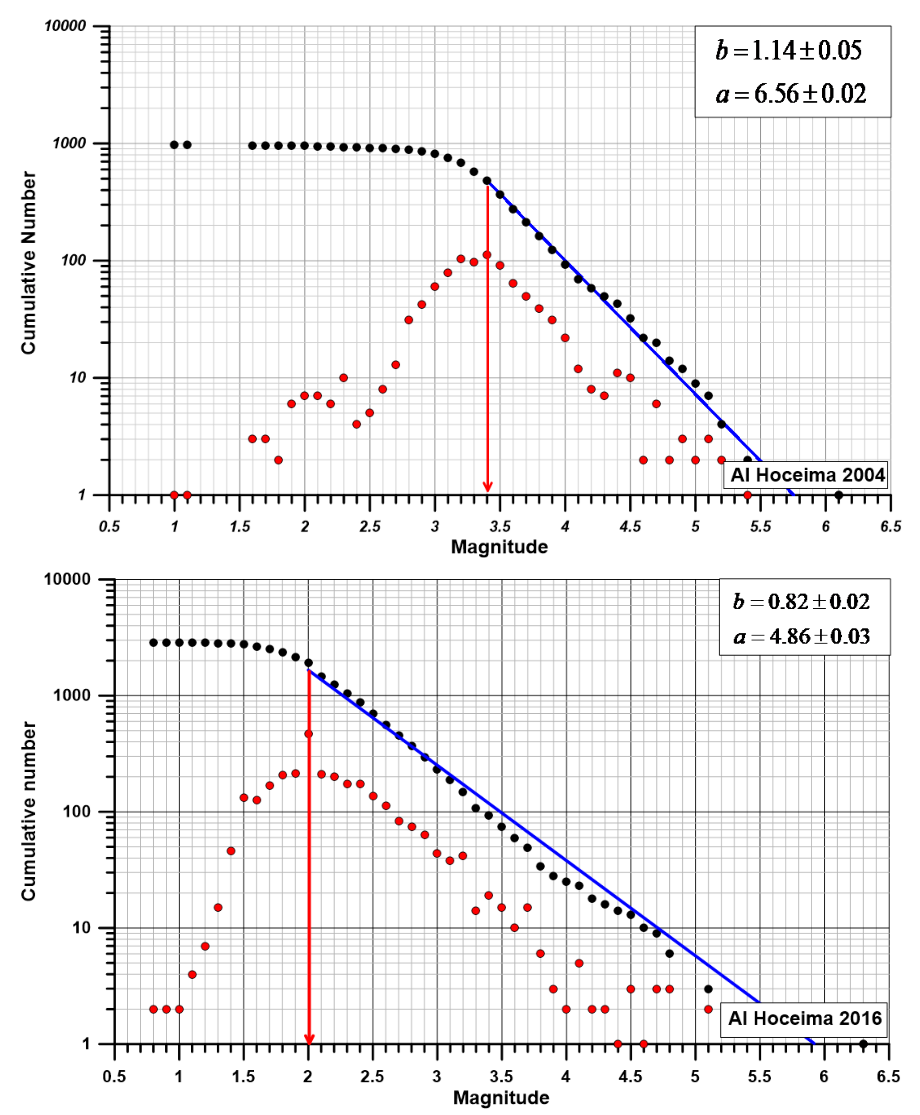
5. Magnitude–Frequency Relationships

The Gutenberg–Richter recurrence relationship [54,55] is a frequently used approach for quantifying seismic activity in each region and has been shown to apply aftershock frequency–magnitude data. The equation is a reasonable approximation of the frequency–magnitude statistics that describe the correlation between earthquake occurrence frequency and magnitude

$${log}_{10} N \left(\ge m\right)=a-bm m\ge m_c$$

(1)

where N (≥m) is the number of events with magnitudes greater than or equal to m. For the estimation of both the a and b-values, it is widely recommended to use a complete dataset for all ranges of magnitude.

The threshold magnitude parameter m_c, is typically determined using one of two methods: a network-based [56,57] or catalog-based approach [56,57]. The first group uses the day-to-night ratio to calculate the earthquake frequency, if noise reduces the detection threshold at night [58,59]. The second set of approaches assumes that earthquake production is self-similar, allowing us to use a power law or the Gutenberg–Richter relationship to construct earthquake frequency–magnitude distributions. The most applied methods in this group reviewed by [60,61] are the maximum curvature (Maxc) method [62], entire magnitude range (EMR) method [60,63], median-based analysis of the segment slope (Mbase) [64], determination of b-value instability [65] and goodness-of-fit test (Gft) by [62], which was later modified by [66].

The threshold magnitude for each of the three sequences under consideration was thoroughly estimated in the current study. Although both the maximum curvature (Maxc), Gft, Gft at levels of 5% and 10% (Gft5% and Gft10%), and modified goodness of fit (mGft) methods were first investigated, the maximum curvature method produced better results, i.e., a better fit (Table 1). Threshold magnitude values of 2.8, 3.4 and 2.0 were obtained for the 1994, 2004 and 2016 aftershock sequences, respectively. The threshold value fluctuated over time, which was also studied. This temporal fluctuation is depicted in Figure 8 and was computed using a sliding-window method.

Prior to each new computation, a window of 20 events was shifted by five events [67]. The middle time of the associated window is supplied to each new threshold magnitude value. The window length was chosen as the balance between the need for temporal resolution and smoothness. Multiple tests were conducted first, changing the number of occurrences per window and the shift; however, neither aspect had a significant influence on the definition. The maximum likelihood approach was used and is considered one of the most reliable approaches for computing the b-value among the available methods. The estimator by [68], given below, was used to calculate the b-value:

$$b=\frac{{log}_{10}e}{\langle m\rangle -m_c}$$

(2)

〈m〉 being the average value of the magnitude. An estimate of the standard deviation σ_b is obtained using the [69] relation, given as follows:

$${\sigma }_b=2.30 b^2\sqrt{\frac{{{\displaystyle \sum }}_{i=1}^N{\left(m_i-m\right)}^2}{N\left(N-1\right)}}$$

(3)

According to [69,70], even when the b-value varies in time and/or space, this relationship provides a reliable approximation of b-uncertainty. When utilizing rounded magnitudes, the estimator by [68] is inaccurate but agrees with the modified distribution of [71]. Then, the improved estimator by [72], given below, is used to determine the maximum likelihood b-value:

$$b=\frac{{log}_{10}e}{\langle m\rangle -\left(m_c-\frac{\Delta m}{2}\right)}$$

(4)

The estimated b-value appraisal for the 1994, 2004 and 2016 aftershock sequences, using the maximum likelihood estimator by [72], with a bin width of 0.1 units, are 1.01 ± 0.07, 1.14 ± 0.05 and 0.82 ± 0.02, respectively (Table 1). Figure 9 shows the power law distributions for the three sequences as fitted by a straight line. The greatest magnitudes, corresponding to the mainshock, are not explained by the Gutenberg–Richter relationship and are thus regarded as outliers in all series. It is worth mentioning that the estimated maximum likelihood parameters are closely linked to and impacted by the previously determined threshold magnitude.

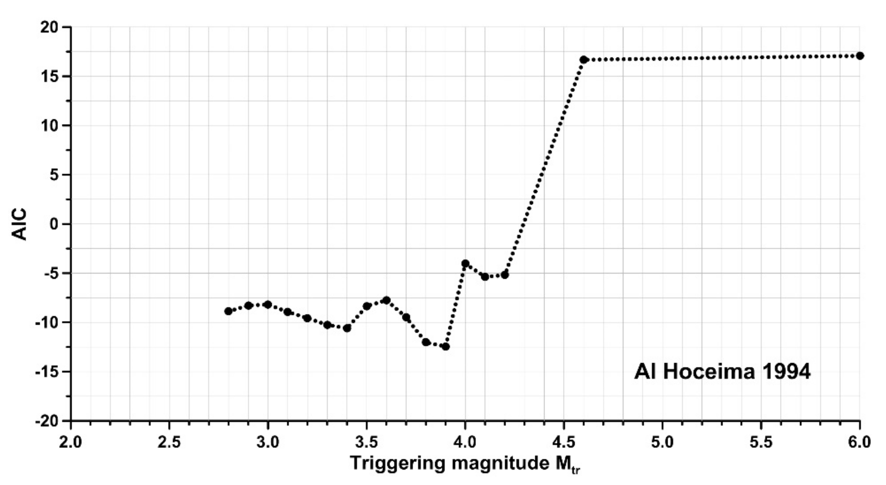
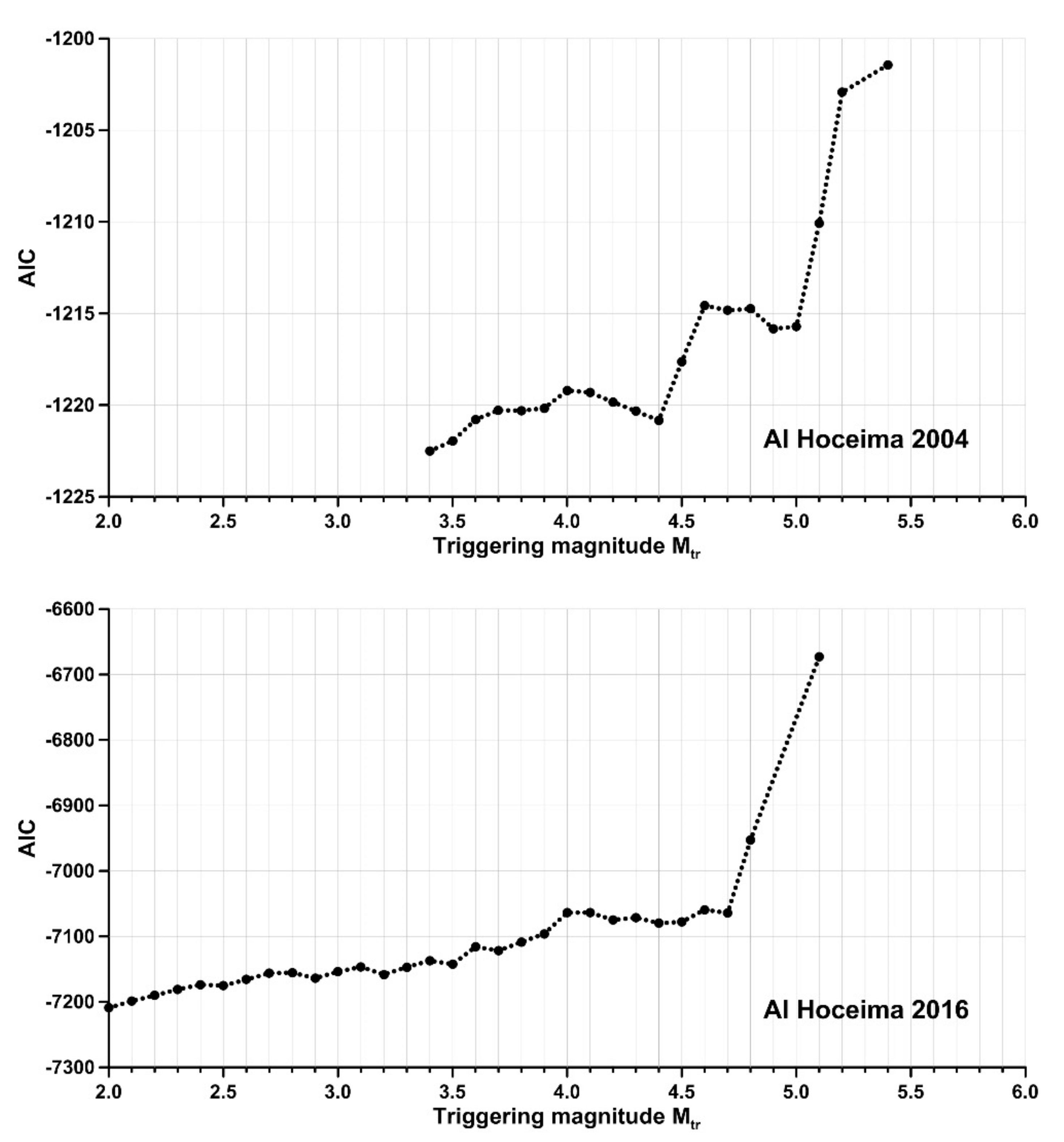
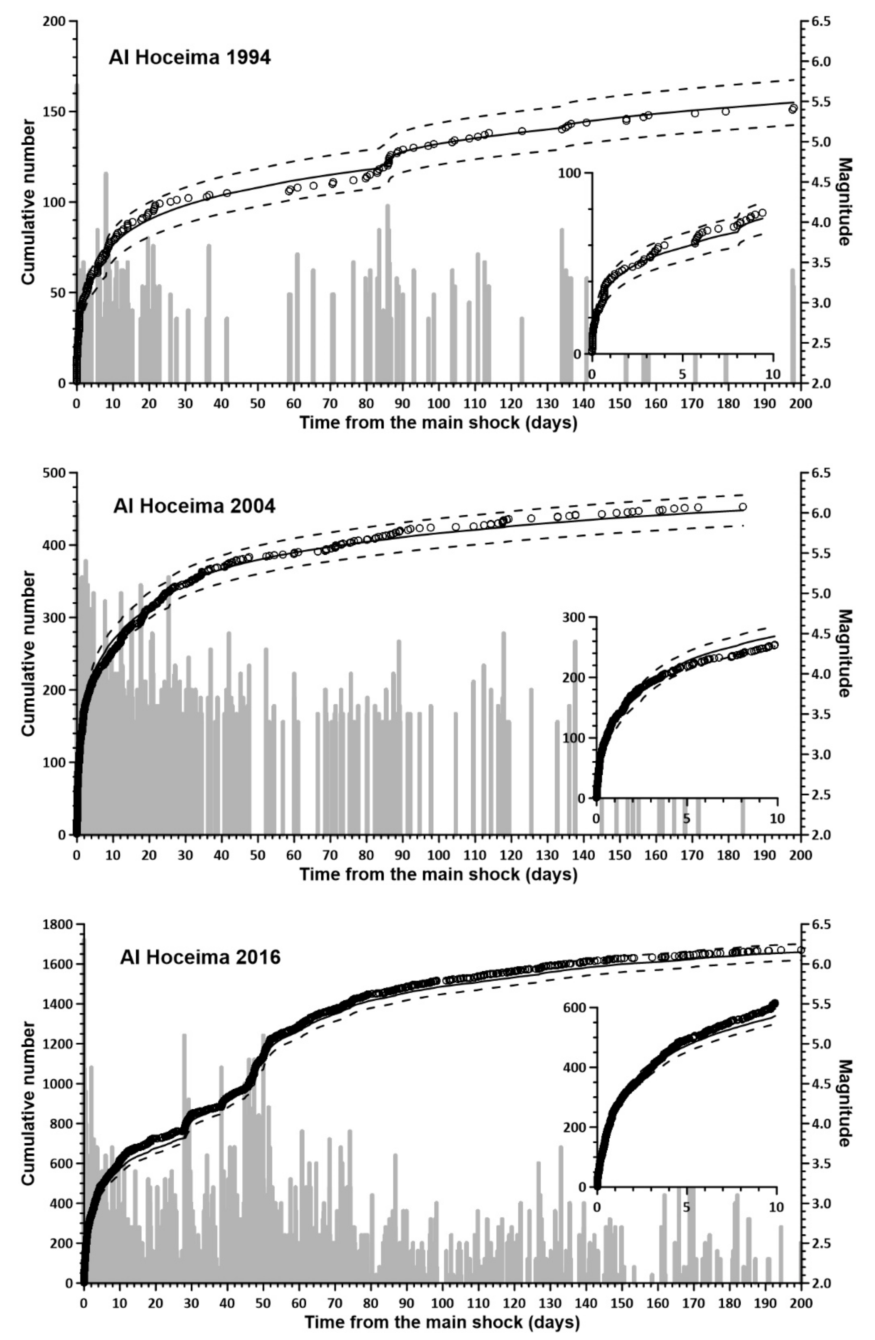
6. Temporal Stochastic Modeling for the Al Hoceima Sequences

This section focuses on the point process modeling of the studied aftershock sequences. Many approaches for modeling this gradual decrease in aftershock frequency have been presented in the literature. The most commonly used model is the Omori law [3], which was improved by [4] into the modified Omori formula (MOF). According to [4], the decay rate of the aftershock per unit time is given as follows:

$$n\left(t\right)=\frac{K}{{\left(t+c\right)}^p}$$

(5)

where t is the time after the occurrence of the mainshock, and the parameter K is related to the mainshock event and threshold magnitude. The c parameter is a debatable number [73,74], with the early stages of imprecise detection of low events in the sequence having a significant effect [75]. Finally, the p parameter is a decay constant, and it is quite likely the most important parameter for understanding the behavior of the sequence. The p-value varies from sequence to sequence and typically ranges from 0.5 to 1.8 [73]. This variation may be related to tectonic activity in the area. However, the elements that influence the p-value remain unclear [76,77].

The quantity n(t) allows us to connect with the point process model by considering it a conditional intensity.

$$n\left(t\right)\approx \mathit{\lambda }\left(t\right),$$

(6)

bearing in mind that [5]:

$$P \left\{an event occurs in \left(t,t+dt\right)|{\Im }_t\right\}=\mathit{\lambda }\left(t|{\Im }_t\right) dt+o\left(dt\right),$$

(7)

where ${\Im }_t$ denotes the internal history of the occurrence process at time t, $\mathit{\lambda }\left(t|{\Im }_t\right)$ is the conditional intensity function [5,78], and o(dt), in the Landau notation, is a function of a lower order than the function λ, i.e., o(dt) being negligible. The MOF model includes only the mainshock occurrence time because it is based on the concept that the entire relaxation process is driven by the stress changes induced by the mainshock alone. The aftershocks are conditionally independent and follow a non-stationary Poisson process.

The MOF model fits data for simple aftershock sequences well; however, secondary clustering is common when there are secondary aftershocks triggered by strong earthquakes in a sequence. The authors in [5] argued that aftershock clustering is a self-similar process in which all aftershocks might induce other aftershocks, with a triggering capacity dependent on their magnitudes, because of these complex situations involving one or more secondary events.

The model was named ETAS, and its conditional intensity function is given as follows [79]:

$$\mathit{\lambda }\left(t|{\Im }_t\right)=\mu +{\displaystyle \sum }_{i; t_i<t}\frac{k_0{e}^{\alpha \left(m_i-m_c\right)}}{{\left(t-t_i+c\right)}^p}$$

(8)

where μ is the background seismicity rate. The internal history ${\Im }_t$ includes the time occurrence t_i (in days after the mainshock) and magnitude events m_i of all the events occurring before time t. The summation includes all events with occurrence times t_i and magnitudes equal to or greater than the lower cut-off m_c. The c and p model parameters were the same as those used in the MOF model. Furthermore, k₀ is a parameter that affects total aftershock productivity and is common to all aftershocks.

According to [80], every term of the summation in Equation (8) indicates the contribution of a prior event to the occurrence probability of subsequent events at time t. The exponential term is controlled by two factors: (a) the temporal rate decrease, as presented by the MOF model and (b) the exponential term chosen because the logarithm of the aftershock area and the magnitude of the mainshock present a linear relationship [81]. Parameter α measures the effect of the magnitude of the production of ‘children’ events, also called “descendants”.

The MOF and ETAS models, as expressed by Equations (5) and (8), respectively, present two limited cases for modeling the temporal distribution of an aftershock sequence. Ref. [2] proposed a similar model, the RETAS model, based on the assumption that not all events in a series; however, only aftershocks with magnitudes greater than or equal to a threshold value, can directly cause the aftershocks of “descendants”. This model allows for the inclusion of all potential models between the two limit cases of the MOF and ETAS models, resulting in the conditional intensity expressed as follows:

$$\mathit{\lambda }\left(t|{\Im }_t\right)=\mu +{\displaystyle \sum }_{\begin{array}{c}i; t_i<t\\ m_i\ge M_{tr}\end{array}}\frac{k_0{e}^{\alpha \left(m_i-m_c\right)}}{{\left(t-t_i+c\right)}^p}$$

(9)

It is worth noting that the RETAS model developed by [8] is based on Bath’s law, which states that the difference between mainshock magnitude and the strongest aftershock magnitude, ranges between 1.2 to 1.4 units. According to this relationship, ref. [8] argued that the difference between the weaker primary event and the weakest event in the aftershock sequence must be at least 1.2 units, by applying this principle to the subsequences generated by the primary trigger model.

Furthermore, the RETAS model has the advantage of examining all potential models between the MOF and ETAS models because the triggering magnitude ranges from the threshold magnitude to the mainshock magnitude. The Akaike information criterion [82], abbreviated as AIC, was used to choose the best-fit model in our case, with the lower AIC value. This is expressed as follows:

$$\mathrm{AIC}=-2 \underset{\theta }{max} log L\left(\theta ;0,T\right)+2k^{”}$$

(10)

where $k^{”}$ represents the number of parameters of the model, and $log L$ is the logarithm of the likelihood function, given as follows:

$$log L\left(\theta ;0,T\right)={\displaystyle \sum }_{i=1}^N{log}_{10}{\mathit{\lambda }}_{\theta }\left(t_i|{\Im }_{t_i}\right)-\underset{0}{\overset{T}{{\displaystyle \int }}}{\mathit{\lambda }}_{\theta }\left(s|{\Im }_s\right)ds$$

(11)

In the previous Equation (12), N is the number of earthquakes with magnitudes greater than or equal to m_c, occurring at times t_j (j = 1, 2, …, N), during [0, T]. Due to the features of the described model, it was used in this study to investigate three aftershock sequences. Table 1 lists the magnitude thresholds used in this study.

As a result of the RETAS model analysis, Figure 10 displays the AIC value versus the triggering magnitude value. Analysis of this curve reveals the aftershock clustering type that is most common in the sequence. The AIC parameter was calculated for all the potential models by varying the triggering magnitude from the threshold magnitude to the magnitude of the mainshock. The best-fit model shows the AIC minimum values in

Table 3. The computed parameters for the RETAS model.

Sequence	Mtr	Best Model	AIC	K0	α	c	p
1994	3.9	RETAS	−12.4	1.727	0.0630	0.024	0.909
2004	3.4	ETAS	−1222.5	3.426	0.0035	0.082	1.070
2016	2.0	ETAS	−7209.0	1.477	0.0380	0.039	1.183

as well as the triggering magnitude and model parameters.

When examining the AIC values vs. $M_{tr}$ curves (Figure 10), we can see that the best-fit model for the minimal AIC value was found to be for a $M_{tr}$ value of 3.9 for the 1994 sequence. For the 2004 sequence, an $M_{tr}$ value of 3.4 is the best-fit model obtained and, for the 2016 sequence, a magnitude of 2.0. The best-fit model became an ETAS model when the triggering magnitude $M_{tr}$ coincided with the completeness threshold magnitude m_c in the last two $M_{tr}$. Analyzing the AIC vs. $M_{tr}$ trigger magnitude curve for the 2016 sequence, a monotonic trend exists, resulting in a continuous increase in AIC values, the lowest of which is for $M_{tr}=m_c$.

According to the model presented in Figure 11, the estimated best model parameters shown in Table 3 were used to compute the expected cumulative number of earthquakes and error bounds. The computed values were compared with the observed cumulative number of earthquakes. Figure 11 shows that the estimated model matches the observed data well for all three sequences, with the observed values remaining inside the error boundaries throughout the whole sequence.

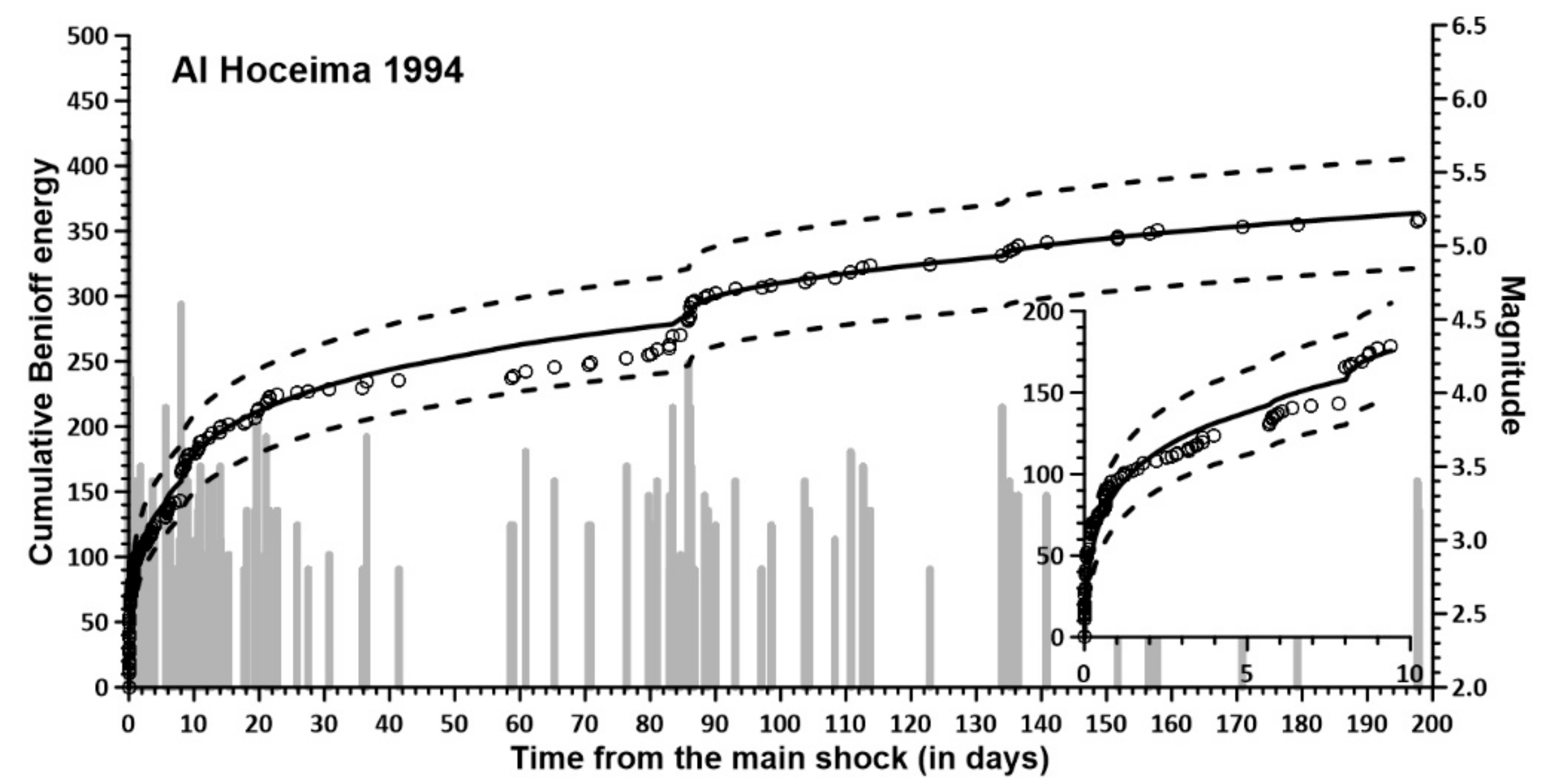
7. Stochastic Model for the Energy Release

In the literature, several attempts have been made to improve earthquake time models by including data on other characteristics associated with event occurrences, such as space-time models or those that relate event occurrence time to a size value of the event (intensity, magnitude or energy). In this context, this section aims to investigate the relationship between the occurrence times {T_k, k = 1,…, n} and released energy {E_k, k = 1,…, n}, providing information on the size of the events in the studied sequences. It is typically considered that the time of occurrence and scale of an event are unrelated.

As a result, our aim was to create an energetic stochastic model that incorporates these considerations and examines how well it represents the observed data. According to [83], marked point processes have similar counting processes [84,85]. The following is a description of this model. Given a Poisson process {N(t); t ≥ 0} with a rate λ > 0, it is assumed that the time T_k of each event is linked to a realization, which is a family {Y_k; k > 0} of independent and identically distributed random variables called marks, with a probability distribution function equal to

$$G\left(y\right)=P\left\{Y_k\le y\right\}$$

(12)

The second requirement is that the random variables are at the same time independent from {N(t); t ≥ 0}. Then, according to [84,85], the stochastic model, typically called the compound Poisson process, is defined as follows:

$$Z\left(t\right)={\displaystyle \sum }_{k=1}^{N\left(t\right)}{Y}_k; t\ge 0$$

(13)

Denoted by μ and γ² are the mean and variance of the marks Y_k; the moments of Z(t) are then given as follows:

$$E\left[Z\left(t\right)\right]=\mathit{\lambda }\mu t$$

(14)

$$var\left[Z\left(t\right)\right]=\mathit{\lambda }\left({\gamma }^2+{\mu }^2\right)t$$

(15)

Consequently, in the case of a series of occurrence times and event sizes, the compound Poisson process can be used as a model process for random behavior. In the most general treatment of a compound point process, {N(t); t ≥ 0} is an inhomogeneous Poisson process with an intensity function {λ(t); t ≥ 0}, and marks {Y_k; k > 0} do not have to form an independent series of random variables. Equations (14) and (15) must be rewritten in the context of an inhomogeneous Poisson process with a rate that varies with time λ = λ(t)

$$E\left[Z\left(t\right)\right]=\mu \underset{t_0}{\overset{t}{{\displaystyle \int }}}\mathit{\lambda }\left(s\right)ds$$

(16)

$$var\left[Z\left(t\right)\right]=\left({\gamma }^2+{\mu }^2\right)\underset{t_0}{\overset{t}{{\displaystyle \int }}}\mathit{\lambda }\left(s\right)ds$$

(17)

The following relationship (18) between the log of the released energy and the magnitude is used [55,86] because the most common way of describing the size of an earthquake is by its magnitude.

$${log}_{10}\sqrt{E}=2.4+0.75 M$$

(18)

The relationship described by this Equation (18), according to [86,87], is consistent with what is expected theoretically for classical crack models with a constant stress drop. This generalized energy–magnitude scaling equation works for various magnitude ranges.

As the cumulative released energy is a physical quantity, it is helpful to consider the series of released energies in the compound Poisson process scheme. It is worth noting that this method has several limitations. First, the energy is determined by the wide dynamic range of the released energy, as well as an instrumentation earthquake record. Thus, to reduce this variability, Equation (18) is transformed as follows:

$$E_k^{tr}=\frac{E_k}{E_0}=\frac{{10}^{4.8+1.5 M_k}}{{10}^{4.8+1.5 M_0}}={10}^{1.5 \left(M_k-M_0\right)}$$

(19)

where E_k and M_k correspond to the energy and magnitude of the k-th event, respectively, and E₀ and M₀ are the energy and magnitude of the first event considered, respectively. $E_k^{tr}$ is the Benioff’s energy.

The approach described above was used to analyze the considered aftershock sequences. Considering the compound Poisson process, given as follows:

$$Z\left(t\right)={\displaystyle \sum }_{k=1}^{N\left(t\right)}{E}_k^{tr}$$

(20)

Equations (16) and (17) were used to derive the estimation of the mean E[Z(t)] and the variance var[Z(t)] for each series, considering the best-fit model derived and analyzed in the previous section. Figure 12 displays the expected cumulative energy and confidence bounds, mean plus/minus the standard deviation, according to the appropriate best-fit model for each aftershock sequence, and this is compared to the computed cumulative energy released in the sequences.

It should be noted that the stochastic model used follows the two previously quoted assumptions: both the independence of the magnitudes and the independence of the magnitudes with the occurrence time. Figure 12 shows that, for the 1994 sequence, no significant deviation of real data values from the model was observed, which supports the above assumptions. However, deviations of the real data values with the model were observed for the two other aftershock sequences.

For the 2004 sequence, the main deviation was observed at the beginning of the sequence, up to the 30th day, where the clustering of stronger aftershocks was recognized. This reveals that the assumption of the independence of magnitudes with occurrence times is not valid in this case. In addition, another deviation of the observed data out of the error bounds can be observed in the 2016 sequence, where an additional concentration of stronger aftershocks is recognized.

8. Discussion

In the present study, the stress pattern analysis revealed that all solutions had a maximum compressive horizontal stress (SHmax) between 142° N and 153° N, which is compatible with previous regional stress data as determined by previous studies. Furthermore, according to these results, the extension directions are clearly compatible with the Betic–Internal Rif’s zone movement southwestward.

The results for all the seismic sequences share horizontal stresses, showing a NW–SE compression and a NE–SW extension as a result of the regional setting. Nonetheless, some significant differences can be observed in the axial ratios and local stress regimes because of the series location in the main shear zone crossing the Alboran Sea and the activated structures in the main and secondary clusters. The three series induced a different fault system, also hosting seismicity, from which the sequence began.

Concerning observed differences in the tectonic characteristics of the series, the 1994 sequence is mainly scattered along a NNE-SSW trending cluster over an almost vertical plane [32], the 2004 sequence is mainly scattered along a NE-SW strike slip fault, and the 2016 sequence is initially scattered along a NNE-SSW trending cluster over a subvertical strike-slip fault, then changing to N-S and finally distributed on a second rounded cluster with a dominant reverse focal mechanism solution [26]. The magnitude of completeness values considered in the current study were compared with those derived using Gft and mGft methods.

Figure 13 shows plots of residuals vs. the minimum magnitudes for the three series. The results obtained matched the estimated values derived using the maximum curvature (Maxc) method. All approaches yield a result of 2.8 for the 1994 series. For the 2004 series, the difference was of the order of 0.1 using mGft, Gft5% and Maxc and 0.2 between Gft10% and Maxc. However, in the case of the 2016 series, the difference varies between 0.2 and 0.3. The results are 1.9 using Gft10%, 2.2 for Gft5%, 2.3 for mGft and 2.0 for Maxc.

As discussed in this study, the RETAS model was used to study the gradual decay of the aftershock frequency based on the triggering magnitude M_tr assumption. The minimum value of the AIC parameter was used as a criterion for selecting the best-fit model. All possible models were estimated by varying the triggering magnitude M_tr from the threshold magnitude m_c (ETAS model) or m_ms (MOL model) to the mainshock magnitude. The results derived for the 1994 and 2004 series highlight and improve on the previous ones derived by [88]. For instance, for the 2004 aftershock sequence, as in [88], the minimum AIC value shows results for the best ETAS model. Considering that the 2016 sequence began on January 21 with an event of Mw 5.1, as suggested by some authors [26], the ETAS model was obtained as the best-fit model.

Stochastic modeling of the energy revealed that the energy released over the series was outlined well by the proposed model in the 1994 and 2004 series. However, there were minor discrepancies in the 2016 sequence and the computed cumulative released energy did not match the model well. We deduced from the analysis that large aftershock clusters occurred more frequently and quickly after the main shock than they would if they occurred at random. This observation holds true for the Zemmouri, Algeria aftershock series of 2003 [88].

9. Conclusions

Stochastic modeling was used to analyze three sequences of events that occurred in Al Hoceima, Morocco, May 1994, February 2004 and January 2016. The analysis of the behavior of the decay rate of the three series, together with the composite stress pattern and the obtained b-value, led us to conclude that the 2016 sequence is the most complex of the three series, likely because of two different fault systems being activated—the main one corresponding to a strike-slip stress and the second one to reverse faults.

The released energy analysis allowed us to characterize the occurrence of large aftershocks shortly after the mainshock better than it would if they occurred at random. However, further research is needed to estimate the recurrence period of such large occurrences, as well as the probability of exceeding a specific magnitude shortly after the mainshocks. This type of research could be conducted in other seismically active regions to investigate the behavior of the seismic series occurring in these areas. This could help to understand the characteristics of the earthquake generation process aimed at seismic forecasting studies.

It should be noted that earthquake forecasting is the ultimate challenge for seismologists because it accumulates scientific knowledge about the earthquake occurrence process and is an essential component of any efficient risk-mitigation strategy [89,90]. As stated by different authors (e.g., [80,91]), RETAS models can be applied to forecast the occurrence probability evolution of a certain sequence, providing the possibility to identify the type of clustering in future seismic series. This is an issue also related to, for instance, the fault distribution and possible fault interactions in the studied area.

References

1. Mogi, K. Some discussions on aftershocks, foreshocks and earthquake swarms. The fracture of a semi-infinite body caused by an inner stress origin and its relation to the earthquake phenomena. Bull. Earthq. Res. Inst. 1963, 41, 615–658. [Google Scholar]
2. Gospodinov, D.; Rotondi, R. Statistical analysis of triggered seismicity in the Kresna region of SW Bulgaria (1904) and the Umbria-Marche region of central Italy (1997). Pure Appl. Geophys. 2006, 163, 1597–1615. [Google Scholar] [CrossRef]
3. Omori, F. On the aftershocks of earthquake. J. Coll. Sci. Imp. Univ. Tokyo 1894, 7, 111–200. [Google Scholar]
4. Utsu, T. A statistical study on the occurrence of aftershocks. Geophys. Mag. 1961, 30, 521–605. [Google Scholar]
5. Ogata, Y. Statistical models for earthquake occurrence and residual analysis for point processes. J. Am. Stat. Assoc. 1988, 83, 9–27. [Google Scholar] [CrossRef]
6. Vere-Jones, D.; Davies, R.B. A statistical survey of earthquakes in the main seismic region of New Zealand. Part 2. Time Series Analyses. N. Z. J. Geol. Geophys. 1966, 9, 251–284. [Google Scholar] [CrossRef]
7. Vere-Jones, D. Stochastic models for earthquake occurrence (with discussion). J. Roy. Statist. Soc. Ser. 1970, 32, 1–62. [Google Scholar]
8. Gospodinov, D.; Rotondi, R. RETAS: A restricted ETAS model inspired by Bath’s law. In Proceedings of the 4th International Workshop on Statistical Seismology, Kanagawa, Japan, 9–13 January 2006. [Google Scholar]
9. Bath, M. Lateral inhomogeneities in the upper mantle. Tectonophysics 1965, 2, 483–514. [Google Scholar] [CrossRef]
10. Bath, M. Introduction to Seismology; BirkhauserVerlag: Basel, Switzerland, 1973; 395p. [Google Scholar]
11. Ogata, Y. Exploratory analysis of earthquake clusters by likelihood-based trigger models. J. Appl. Probab. 2001, 38A, 202–212. [Google Scholar] [CrossRef]
12. Console, R.; Lombardi, A.M.; Murru, M.; Rhoades, D. Båth’s law and the self-similarity of earthquakes. J. Geophys. Res. 2003, 108, 2128. [Google Scholar] [CrossRef]
13. Hamdache, M.; Henares, J.; Peláez, J.A.; Damerdji, J. Fractal analysis of earthquake sequences in the Ibero-Maghrebian region. Pure Appl. Geophys. 2019, 176, 1379–1416. [Google Scholar] [CrossRef]
14. Panzera, F.; Zechar, J.D.; Vogfjörd, K.S.; Eberhard, D.A.J. A revised earthquake catalogue for South Iceland. Pure Appl. Geophys. 2015, 173, 97–116. [Google Scholar] [CrossRef]
15. Chalouan, A.; Michard, A.; El Kadiri, K.; Negro, F.; de Lamotte, D.F.; Soto, J.I.; Saddiqi, O. The Rif Belt. In Continental Evolution: The Geology of Morocco. Lecture Notes in Earth Sciences; Michard, A., Saddiqi, O., Chalouan, A., Lamotte, D.F., Eds.; Springer: Berlin/Heidelberg, Germany, 2008; Volume 116, pp. 203–302. [Google Scholar]
16. Comas, M.C.; García-Dueñas, V.; Jurado, M.J. Neogene tectonic evolution of the Alboran Sea from MCS data. Geo. Mar. Lett. 1992, 12, 157–164. [Google Scholar] [CrossRef]
17. Boillot, G.; Montadert, L.; Lemoine, M.; Biju-Duval, B. Les Margescontinentales Actuelles et Fossiles Autour de la France; Elsevier Masson: Amsterdam, The Netherlands, 1984; 352p. [Google Scholar]
18. De Mets, C.; Gordon, R.G.; Argus, D.F. Geologically current plate motions. Geophys. J. Int. 2010, 181, 1–80. [Google Scholar] [CrossRef] [Green Version]
19. Peláez, J.A.; Henares, J.; Hamdache, M.; Sanz de Galdeano, C. A seismogenic zone model for seismic hazard studies in Northwestern Africa. In Moment Tensor Solutions. A Useful Tool for Seismotectonics; D’Amico, S., Ed.; Springer Natural Hazards: Berlin/Heidelberg, Germany, 2018; pp. 643–680. [Google Scholar]
20. Sparacino, F.; Palano, M.; Peláez, J.A.; Fernández, J. Geodetic deformation versus seismic crustal moment-rates: Insights from the Ibero-Maghrebian region. Remote Sens. 2020, 12, 952. [Google Scholar] [CrossRef]
21. Pedrera, A.; Ruiz Constán, A.; Galindo-Zaldívar, J.; Chalouan, A.; Sanz de Galdeano, C.; Marín Lechado, C.; Ruano, P.; Benmakhlouf, M.; Akil, M.; López Garrido, C.; et al. Is there an active subduction beneath the Gibraltar orogenic arc? Constraints from Pliocene to present-day stress field. J. Geodyn. 2011, 52, 83–96. [Google Scholar] [CrossRef]
22. Martínez-García, P.; Comas, M.; Lonergan, L.; Watts, A.B. From extension to shortening: Tectonic inversion distributed in time and space in the Alboran Sea, western Mediterranean. Tectonics 2017, 36, 2777–2805. [Google Scholar] [CrossRef]
23. Larouzière, F.; Bolze, J.; Bordet, P.; Hernández, J.; Montenat, C.; Ott d’Estevou, P. The Betic segment of the lithospheric Trans-Alboran shear zone during the Late Miocene. Tectonophysics 1988, 152, 41–52. [Google Scholar] [CrossRef]
24. Benkmakhlouf, M.; Galindo-Zaldívar, J.; Chalouan, A.; Sanz de Galdeano, C.; Ahmamou, M.; López-Garrido, A.C. Inversion of transfer faults: The Jebha-Chrafate fault (Rif, Morocco). J. Afr. Earth Sci. 2012, 73–74, 33–43. [Google Scholar] [CrossRef]
25. Sautkin, A.; Talukder, A.R.; Comas, M.C.; Soto, J.I.; Alekseev, A. Mud volcanoes in the Alboran Sea: Evidence from micro paleontological and geophysical data. Mar. Geol. 2003, 195, 237–261. [Google Scholar] [CrossRef]
26. Galindo Zaldívar, J.; Ercilla, G.; Estrada, F.; Catalán, M.; d’Acremont, E.; Azzouz, O.; Casas, D.; Chourak, M.; Vázquez, J.T.; Chalouan, A.; et al. Imaging the growth of recent faults: The case of 2016–2017 seismic sequence sea bottom deformation in the Alboran Sea (western Mediterranean). Tectonics 2018, 37, 2513–2530. [Google Scholar] [CrossRef]
27. Stich, D.; Mancilla, F.; Baumont, D.; Morales, J. Source analysis of the Mw 6.3 2004 Al Hoceima earthquake (Morocco) using regional apparent source time functions. J. Geophys. Res. 2005, 110, B06306. [Google Scholar]
28. Akoglu, M.; Cakir, Z.; Meghraoui, M.; Belabbes, S.; El Alami, S.O.; Ergintav, S.; Akyuz, H.S. The 1994–2004 Al Hoceima (Morocco) earthquake sequence: Conjugate fault ruptures deduced from InSAR. Earth Planet. Sci. Lett. 2006, 252, 467–480. [Google Scholar] [CrossRef]
29. Biggs, J.; Bergman, E.; Emmerson, B.; Funning, G.J.; Jackson, J.; Parson, B.; Wright, T.J. Fault identification for buried strike-slip earthquakes using INSAR: The 1994 and 2004 Al Hoceima, Morocco earthquakes. Geophys. J. Int. 2006, 166, 1347–1362. [Google Scholar] [CrossRef]
30. Galindo Zaldívar, J.; Chalouan, A.; Azzouz, O.; Sanz de Galdeano, C.; Anahnah, F.; Ameza, L.; Ruano, P.; Pedrera, A.; Ruiz-Constan, A.; Marín-Lechado, C.; et al. Are seismological and geological observations of the Al Hoceima (Morocco Rif) 2004 earthquake (M=6.3) contradictory? Tectonophysics 2009, 475, 59–67. [Google Scholar] [CrossRef]
31. Galindo Zaldívar, J.; Azzouz, O.; Chalouan, A.; Pedrera, A.; Ruano, P.; Ruiz Constán, A.; Sanz de Galdeano, C.; Marín Lechado, C.; López Garrido, A.C.; Anahnah, F.; et al. Extensional tectonics, graben development and fault terminations in the Eastern Rif (Bokoya-Ras Afrou área). Tectonophysics 2015, 663, 140–149. [Google Scholar] [CrossRef]
32. El Alami, S.O.; Tadili, B.A.; Cherkaoui, T.E.; Medina, F.; Ramdani, M.; Aït Brahim, L.; Harnafi, M. The Al Hoceima earthquake of May 26, 1994 and its aftershocks: A seismotectonic study. Ann. Geophys. 1998, 41, 519–537. [Google Scholar] [CrossRef]
33. Medina, F.; Cherkaoui, T.E. The south-western Alboran earthquake sequence of January-March 2016 and its associated coulomb stress changes. Open J. Earthq. Res. 2017, 26, 35–54. [Google Scholar] [CrossRef]
34. Van der Woerd, J.; Dorbath, C.; Ousadou, F.; Dorbath, L.; Delouis, B.; Jacques, E.; Tapponnier, P.; Hahou, Y.; Menzhi, M.; Frogneux, M.; et al. The Al Hoceima Mw 6.4 earthquake of 24 February 2004 and its aftershocks sequence. J. Geodyn. 2014, 77, 89–109. [Google Scholar] [CrossRef]
35. Kariche, J.; Meghraoui, M.; Timoulali, Y.; Cetin, E.; Toussaint, R. The Al Hoceima earthquake sequences of 1994, 2004 and 2016: Stress transfer and poroelasticity in the Rif and Alboran Sea region. Geophys. J. Int. 2018, 212, 42–53. [Google Scholar] [CrossRef]
36. Buforn, E.; Pro, C.; Sanz de Galdeano, C.; Cantavella, J.V.; Cesca, S.; Caldeira, B.; Udías, A.; Mattesini, M. The 2016 south Alboran earthquake (Mw = 6.4): A reactivation of the Ibero-Maghrebian region? Tectonophysics 2017, 712, 704–715. [Google Scholar] [CrossRef]
37. López Casado, C.; Garrido, J.; Delgado, J.; Peláez, J.A.; Henares, J. HVSR estimation of site effects in Melilla (Spain) and the damage pattern from the 01/25/2016 Mw 6.3 Alborán Sea earthquake. Nat. Hazards 2018, 93, S153–S167. [Google Scholar] [CrossRef]
38. Mezcua, J.; Rueda, J. Seismological evidence for a delamination process in the lithosphere under the Alboran Sea. Geophys. J. Int. 1997, 129, F1–F8. [Google Scholar] [CrossRef]
39. Medina, F.; El Alami, S.O. Focal Mechanisms and State of Stress in the Al Hoceima Area. Bull. L’institut Sci. Sect. Sci. Terre 2006, 28, 19–30. [Google Scholar]
40. Thio, H.K.; Song, X.; Saikia, C.; Helmberger, D.V.; Woods, B.B. Seismic source and structure estimation in the western Mediterranean using sparse broadband network. J. Geophys. Res. 1999, 104, 845–861. [Google Scholar] [CrossRef]
41. Bezzeghoud, M.; Buforn, E. Source parameters of the 1992 Melilla (Spain, MW = 4.8), 1994 Alhoceima (Morocco, MW = 5.8) and 1994 Mascara (Algeria, MW = 5.7) earthquakes and seismotectonic implications. Bull. Seism. Soc. Am. 1999, 89, 359–372. [Google Scholar]
42. Delvaux, D.; Sperner, B. New aspects of tectonic stress inversion with reference to the TENSOR program. Geol. Soc. Lond. Spec. Publ. 2003, 212, 75–100. [Google Scholar] [CrossRef] [Green Version]
43. Angelier, J.; Mechler, P. Sur une méthode graphique de recherche des contraintes principales également utilisable en tectonique et en sismologie: La méthode des diédres droits. Bull. Soc. Géol. France XIX 1977, 7, 1309–1318. [Google Scholar] [CrossRef]
44. Delvaux, D.; Barth, A. African stress pattern from formal inversion of focal mechanism data. Tectonophysics 2010, 482, 105–128. [Google Scholar] [CrossRef]
45. Hussein, H.M.; AbouElenean, K.M.; Marzou, I.A.; El-Nader, L.F.; Ghazala, H.; El Gabry, M.N. Present-day tectonic stress regime in Egypt and surrounding area based on inversion of earthquake focal mechanism. J. Afr. Earth. Sci. 2013, 81, 1–15. [Google Scholar] [CrossRef]
46. Gephart, J.W.; Forsyth, D.W. An improved method for determining the regional stress tensor using earthquake focal mechanism data: Application to the San Fernando earthquake sequence. J. Geophys. Res. 1984, 89, 9305–9320. [Google Scholar] [CrossRef]
47. Soumaya, A.; Ben Ayed, N.; Delvaux, D.; Ghanmi, M. Spatial variation of present-day stress field and tectonic regime in Tunisia and surroundings from formal inversion of focal mechanisms: Geodynamic implications for central Mediterranean. Tectonics 2015, 34, 1154–1180. [Google Scholar] [CrossRef]
48. Sawires, R.; Peláez, J.A.; Ibrahim, H.A.; Fat Helbary, R.E.; Henares, J.; Hamdache, M. Delineation and characterization of a new seismic source model for seismic hazard studies in Egypt. Nat. Hazards 2016, 80, 1823–1864. [Google Scholar] [CrossRef]
49. Hamdache, M.; Peláez, J.A.; Gospodinov, D.; Henares, J. Statistical features of the 2010 Beni-Ilmane, Algeria, aftershock sequence. Pure Appl. Geophys. 2018, 175, 773–792. [Google Scholar] [CrossRef]
50. Henares, J.; López Casado, C.; Sanz de Galdeano, C.; Delgado, J.; Peláez, J.A. Stress field in the Ibero-Maghrebianregion. J. Seismol. 2003, 7, 65–78. [Google Scholar] [CrossRef]
51. Sanz de Galdeano, C. Geologic evolution of the Betic Cordilleras in the Western Mediterranean, Miocene to the present. Tectonophysics 1990, 172, 107–119. [Google Scholar] [CrossRef]
52. Sanz de Galdeano, C. The E-W segments of the contact between the External and Internal Zones of the Betic and Rif Cordilleras and the E-W corridors of the Internal Zone (A combined explanation). Estudios Geológicos 1996, 52, 123–136. [Google Scholar] [CrossRef]
53. Galindo Zaldívar, J.; Jabaloy, A.; Serrano, I.; Morales, J.; González Lodeiro, F.; Torcal, F. Recent and present-day stresses in the Granada Basin (Betic Cordilleras): Example of a late Miocene-present-day extensional basin in a convergent plate boundary. Tectonics 1999, 18, 686–702. [Google Scholar] [CrossRef]
54. Gutenberg, B.; Richter, C.F. Frequency of Earthquake in California. Bull. Seismol. Soc. Am. 1944, 34, 185–188. [Google Scholar] [CrossRef]
55. Gutenberg, B.; Richter, C.F. Seismicity of the Earth; Princeton University Press: Princeton, NJ, USA, 1954; 310p. [Google Scholar]
56. Schorlemmer, D.; Woessner, J. Probability of detecting anearthquake. Bull. Seismol. Soc. Am. 2008, 98, 2103–2117. [Google Scholar] [CrossRef]
57. Mignan, A.; Werner, M.J.; Wiemer, S.; Chen, C.C.; Wu, Y.M. Bayesian estimation of the spatially varying completeness magnitude of earthquake catalogs. Bull. Seismol. Soc. Am. 2011, 101, 1371–1385. [Google Scholar] [CrossRef]
58. Rydelek, P.A.; Sacks, I.S. Testing the completeness of earthquake catalogs and the hypothesis of self-similarity. Nature 1989, 337, 251–253. [Google Scholar] [CrossRef]
59. Taylor, D.W.A.; Snoke, J.A.; Sacks, I.S.; Takanami, T. Non-linear frequency-magnitude relationship for the Hokkaido corner, Japan. Bull. Seismol. Soc. Am. 1990, 80, 605–609. [Google Scholar] [CrossRef]
60. Woessner, J.; Wiemer, S. Assessing the quality of earthquake catalogs: Estimating the magnitude of completeness and its uncertainty. Bull. Seismol. Soc. Am. 2005, 95, 684–698. [Google Scholar] [CrossRef]
61. Mignan, A.; Woessner, J. Estimating the Magnitude of Completeness for Earthquake Catalogs; Community Online Resource for Statistical Seismicity Analysis: 2012; 45p. Available online: http://www.corssa.org/en/articles/overview/ (accessed on 27 August 2022).
62. Wiemer, S.; Wyss, M. Minimum magnitude of completeness in earthquake catalogs: Examples from Alaska, the Western United States, and Japan. Bull. Seismol. Soc. Am. 2000, 90, 859–869. [Google Scholar] [CrossRef]
63. Ogata, Y.; Katsura, K. Analysis of the temporal and spatial heterogeneity of magnitude frequency distribution inferred from earthquake catalogs. Geophys. J. Int. 1993, 113, 727–738. [Google Scholar] [CrossRef]
64. Amorese, D. Applying a change-point detection method on frequency-magnitude distribution. Bull. Seismol. Soc. Am. 2007, 97, 1742–1749. [Google Scholar] [CrossRef]
65. Cao, A.M.; Gao, S.S. Temporal variation of seismic b-values beneath northeastern Japan island arc. Geophys. Res. Lett. 2002, 29, 48-1–48-3. [Google Scholar] [CrossRef]
66. Leptokaropoulos, K.M.; Karakostas, V.G.; Papadimitriou, E.E.; Adamaki, A.K.; Tan, O.; İnan, S. A Homogeneous Earthquake Catalog for Western Turkey and Magnitude of Completeness Determination. Bull. Seismol. Soc. Am. 2013, 103, 2739–2751. [Google Scholar] [CrossRef]
67. Wiemer, S. A software package to analyze seismicity: Zmap. Seismol. Res. Lett. 2001, 72, 373–382. [Google Scholar] [CrossRef]
68. Aki, K. Maximum likelihood estimate of b in the formula Log N = a − bM and its confidence limits. Bull. Earthq. Res. Inst. Tokyo Univ. 1965, 43, 237–239. [Google Scholar]
69. Shi, Y.; Bolt, B.A. The standard error of the magnitude frequency b value. Bull. Seismol. Soc. Am. 1982, 72, 1677–1687. [Google Scholar] [CrossRef]
70. Marzocchi, W.; Sandri, L. A review and new insights on the estimation of the b-value and its uncertainty. Ann. Geophys. 2003, 46, 1271–1282. [Google Scholar]
71. Márquez-Ramírez, V.H.; Nava, F.A.; Zúñiga, F.R. Correcting the Gutenberg-Richter b value for effects of rounding and noise. Earthq. Sci. 2015, 28, 129–134. [Google Scholar] [CrossRef]
72. Utsu, T. A method for determining the value of b in theformula Log n = a − bm showing the magnitude-frequency relation for earthquakes. Geophys. Bull. Hokkaido Univ. 1965, 13, 99–103. (In Japanese) [Google Scholar]
73. Utsu, T.; Ogata, Y.; Matsu’ura, R.S. The centenary of the Omori formula for a decay law of aftershock activity. J. Phys. Earth 1995, 43, 1–33. [Google Scholar] [CrossRef]
74. Enescu, B.; Mori, J.; Masatoshi, M.; Kano, Y. Omori-Utsu law c-values associated with recent moderate earthquakes in Japan. Bull. Seismol. Soc. Am. 2009, 99, 884–891. [Google Scholar] [CrossRef]
75. Kisslinger, C.; Jones, L.M. Properties of aftershocks in Southern California. J. Geophys. Res. 1991, 96, 11947–11958. [Google Scholar] [CrossRef]
76. Nyffengger, P.; Frolich, C. Recommendations for determining p values for aftershock sequence and catalogs. Bull. Seismol. Soc. Am. 1998, 88, 1144–1154. [Google Scholar]
77. Nyffengger, P.; Frolich, C. Aftershock occurrence rate decay properties for intermediate and deep earthquake sequences. Geophys. Res. Lett. 2000, 27, 1215–1218. [Google Scholar] [CrossRef]
78. Daley, D.J.; Vere Jones, D. An Introduction to the Theory of Point Processes. Vol. I. Elementary Theory and Methods; Springer: Berlin/Heidelberg, Germany, 2003; 471. [Google Scholar]
79. Zhuang, J.; Werner, M.J.; Hainzl, S.; Harte, D.; Zhou, S. Basic Models of Seismicity: Spatiotemporal Models; Community Online Resource for Statistical Seismicity Analysis. 2011. Available online: http://www.corssa.org/en/articles/overview/ (accessed on 27 August 2022).
80. Gospodinov, D.; Karakostas, V.; Papadimitriou, E. Seismicity rate modeling for prospective stochastic forecasting. The case of 2014 Kefalonia, Greece, seismic excitation. Nat. Hazards 2015, 79, 1039–1058. [Google Scholar] [CrossRef] [Green Version]
81. Utsu, T. Seismological evidence for anomalous structure of island arcs with special reference to the Japanese region. Rev. Geophys. 1971, 9, 839–890. [Google Scholar] [CrossRef]
82. Akaike, H. A new look at the statistical model identification. IEEE Trans. Autom. Control 1974, 19, 716–723. [Google Scholar] [CrossRef]
83. Gospodinov, D.; Rotondi, R. Exploratory analysis of marked Poisson processes applied to Balkan earthquake sequences. J. Balkan Geophys. Soc. 2001, 4, 61–68. [Google Scholar]
84. Ross, S.M. Introduction to Probability Models; Academic Press: Berkeley, CA, USA, 2010; 842p. [Google Scholar]
85. Taylor, H.M.; Karlin, S. An Introduction to Stochastic Modeling; Academic Press: Cambridge, MA, USA, 1984; 410p. [Google Scholar]
86. Tzanis, A.; Vallianatos, F. Distributed power-law seismicity changes and crustal deformation in the SW Hellenic arc. Nat. Hazards Earth Syst. Sci. 2003, 3, 179–195. [Google Scholar] [CrossRef]
87. Kanamori, H.; Anderson, D.L. Theoretical basis of some empirical relations in seismology. Bull. Seismol. Soc. Am. 1975, 65, 1073–1095. [Google Scholar]
88. Hamdache, M.; Peláez, J.A.; Talbi, A. Scaling properties of aftershock sequences in Algeria Morocco Region. In Earthquake Research and Analysis—New Advances in Seismology; D’Amico, S., Ed.; Intech Open: London, UK, 2013. [Google Scholar] [CrossRef]
89. Marzocchi, W.; Taroni, M.; Falcone, G. Earthquake forecasting during the complex Amatrice-Norcia seismic sequence. Sci. Adv. 2017, 3, e1701239. [Google Scholar] [CrossRef]
90. Jordan, T.H.; Chen, Y.-T.; Gasparini, P.; Madariaga, R.; Main, I.; Marzocchi, W.; Papadopoulos, G.; Sobolev, G.; Yamaoka, K.; Zschau, J. Operational earthquake forecasting. State of knowledge and guidelines for utilization. Ann. Geophys. 2011, 54, 4. [Google Scholar] [CrossRef]
91. Gospodinov, D.; Papadimitriou, E.E.; Karakostas, V.G.; Ranguelov, B. Analysis of relaxation temporal patterns in Greece through the RETAS model approach. Phys. Earth Planet. Int. 2007, 165, 158–175. [Google Scholar] [CrossRef] [Green Version]
Figure 1. Geologic sketch map of the Betic-Rif region and location of the Al Hoceima study area. Bk: Bokoya Massif; Ra: Ras Afrou; Rt: Tas Tarf; Tf: Tres Forcas Cape. Internal Zone includes Sebtides and Ghomarides in the Rif and Nevado-Filabrides, Alpujarrides and Malaguides in the Betics.
Applsci 12 08744 g001
Figure 2. Seismicity recorded by the Spanish IGN included in the 1994, 2004 and 2016 seismic series from magnitude 2.0. Main tectonic features are displayed.
Applsci 12 08744 g002
Figure 3. Temporal evolution of the studied series (magnitudes above 2.0). Starting of the x-axis does not always correspond to the occurrence of the main event.
Applsci 12 08744 g003
Figure 4. (A) 1994 seismic sequence showing earthquakes with magnitude above 3.0 and computed focal mechanisms for aftershocks [32]. (B) Different focal mechanism solutions for the mainquake. GCMT: Global Centroid Moment Tensor; T&al.: [40]; M&R: [38]; ISC: International Seismological Centre; B&B-I and B&B-II: [41], for a pre-event and the main quake, respectively; B&al.: [29]; EA&al.: [32,39].
Applsci 12 08744 g004
Figure 5. (A) 2004 seismic sequence showing earthquakes with magnitude above 3.0 and computed focal mechanisms for the biggest events. (B) Earthquakes with magnitude above 1.0 and focal mechanism solutions for the biggest events (mb 1.9–3.0) of the “eastern cluster” studied by [34].
Applsci 12 08744 g005
Figure 6. 2016 seismic sequence showing earthquakes with magnitude above 3.0 and computed focal mechanisms.
Applsci 12 08744 g006
Figure 7. Stress regime computed from focal mechanisms. (A) For the 1994 mainshock, (B) for the 1994 aftershock sequence, (C) for the 2004 aftershock sequence, (D) for the ‘eastern cluster’ considered by [34], (E) for the 2016 ‘main cluster’ and (F) for the 2016 ‘secondary cluster’.
Applsci 12 08744 g007
Figure 8. Temporal evolution of the threshold magnitude for the three sequences.
Applsci 12 08744 g008
Figure 9. The cumulative number of earthquakes vs. magnitude (black points and linear fits) and the non-cumulative number of earthquakes (open points) for the three sequences. The threshold magnitude is highlighted.
Applsci 12 08744 g009aApplsci 12 08744 g009b
Figure 10. The AIC values of the RETAS model vs. the triggering magnitude for the three sequences.
Applsci 12 08744 g010aApplsci 12 08744 g010b
Figure 11. The cumulative number of events above magnitude mc for the three sequences. Circles: observed values. Lines: mean ±σ fitted model. The magnitudes of the events included in the sequences are also depicted. Inset stand out the first ten days of the series.
Applsci 12 08744 g011
Figure 12. Cumulative released energy for the three sequences. Circles: observed values. Lines: mean ± σ fitted model. Magnitudes of the events included in the sequences are also depicted. The inset shows the first ten days of the series.
Applsci 12 08744 g012aApplsci 12 08744 g012b
Figure 13. The obtained residuals vs. magnitude when fitting the observed data to the mGft power law (solid line) and theoretical distribution power law (dashed line). The 5% and 10% residual levels are shown as reference.
Applsci 12 08744 g013