Article

Poisson Extended Exponential Distribution with Associated INAR(1) Process and Applications

by
Radhakumari Maya
1,
Christophe Chesneau
2,*,
Anuresha Krishna
3 and
Muhammed Rasheed Irshad
3
1
Department of Statistics, Government College for Women, Trivandrum 695 014, Kerala, India
2
Department of Mathematics, Université de Caen Basse-Normandie, F-14032 Caen, France
3
Department of Statistics, Cochin University of Science and Technology, Cochin 682 022, Kerala, India
*
Author to whom correspondence should be addressed.
Stats 2022, 5(3), 755-772; https://doi.org/10.3390/stats5030044
Submission received: 8 July 2022 / Revised: 23 July 2022 / Accepted: 3 August 2022 / Published: 5 August 2022

Abstract

:
The significance of count data modeling and its applications to real-world phenomena have been highlighted in several research studies. The present study focuses on a two-parameter discrete distribution that can be obtained by compounding the Poisson and extended exponential distributions. It has tractable and explicit forms for its statistical properties. The maximum likelihood estimation method is used to estimate the unknown parameters. An extensive simulation study was also performed. In this paper, the significance of the proposed distribution is demonstrated in a count regression model and in a first-order integer-valued autoregressive process, referred to as the INAR(1) process. In addition to this, the empirical importance of the proposed model is proved through three real-data applications, and the empirical findings indicate that the proposed INAR(1) model provides better results than other competitive models for time series of counts that display overdispersion.

1. Introduction

In many fields of applied sciences, such as engineering, medicine, insurance, economics, and marketing, studying and analyzing count data play a significant role. Count data sets are often modeled using a Poisson distribution. However, the Poisson distribution cannot handle overdispersed data sets. Overdispersion occurs when the variance exceeds the mean. As a consequence, many researchers have developed mixed-Poisson distributions to provide alternative models for overdispersed count data, including [1,2,3,4]. Recent studies in this area are [5,6,7], among others. When using count data as a response variable, Poisson regression is a popular model. It is assumed that the dependent variable’s mean and variance are both identical in the Poisson regression model. There is a lot of evidence to support the overdispersion that the count data sets exhibit. Thus, the Poisson regression’s theoretical premise is practically violated. In the beginning, negative binomial regression (NB) was employed to model overdispersion in the context of count regression. The Poisson-transmuted exponential linear model was introduced by [2] and applied to healthcare data sets. The generalized Poisson–Lindley linear model was introduced by [8], who showed that generalized Poisson–Lindley linear models provide better modeling abilities than Poisson and NB regression models when there is an overdispersion of data.
There are many instances of integer-valued time series in the real world, such as the number of births at a hospital in successive months, the number of accidents, the number of patients, the number of chromosome exchanges in cells, and so on. As an inaugural approach, refs. [9,10,11] proposed a stochastic model for integer-valued time series called INAR(1)P for a first-order non-negative integer-valued autoregressive process with Poisson innovations. As time series of counts mostly exhibit overdispersion, the Poisson distribution is no longer applicable to the INAR(1) process. To overcome this issue, researchers have proposed different INAR(1) processes with flexible innovation distributions. Consequently, Aghababaei Jazi et al. [12] proposed an INAR(1) process with geometric innovations (INAR(1)G), Altun E. [5] presented an INAR(1) process with new Poisson weighted exponential innovation distribution (INAR(1)PWE),Altun et al. [13] introduced an INAR(1) process with Poisson quasi-xgamma innovations (INAR(1)PQX), and so on. Although these methods are excellent for overdispersed time series count data sets, they have significant drawbacks in real-world applications. By discovering more INAR(1) models, more opportunities will be available for optimally fitting real data sets by choosing those models that are most appropriate for each situation.
Therefore, this paper provide new facts on what we call a two-parameter mixed-Poisson distribution, namely the Poisson extended exponential (PEE) distribution, obtained by compounding the Poisson distribution with the extended exponential (EE) distribution proposed by [14]. The EE distribution is obtained by mixing exponential and gamma distributions. The probability density function (pdf) of the EE distribution is given by
f ( x ) = α 2 ( 1 + β x ) e α x α + β , x > 0 , α > 0 , β 0 .
It is sometimes denoted as EE ( α , β ) to specify the parameters. This distribution also appears in a different form in [15], presented as a two-parameter Lindley distribution. Recent statistical literature has paid a lot of attention to the EE distribution. As a result of this, an EE regression model was proposed by [16] in which the reparameterization of the EE model based on the mean is performed. In addition, de Andrade et al. [17] proposed the exponentiated generalized EE distribution. Refs. [18,19] also showed the novelty and possibility of EE distribution through their study of different generalizations of the EE model. The PEE distribution appears in [20] under a discrete two-parameter Poisson–Lindley distribution version. However, to the best of our knowledge, some of these aspects are understudied, and the goal of this research is to rehabilitate them from applied perspectives. In particular, the appealing applicability and competence of the EE regression model inspired us to present a two-parameter mixed-Poisson distribution created by compounding Poisson with the EE distribution and elucidating its regression characteristics and associated INAR(1) process.
In the rest of the paper, the sections are arranged as follows. Section 2 presents the PEE distribution and explores some of its statistical properties. The finite sample performance of the estimation method is examined in Section 3 with a simulation study for the maximum likelihood estimation of the model parameters. A regression model is discussed in Section 4. The INAR(1)PEE process is developed in Section 5 using PEE innovations. An empirical analysis of three real data sets is conducted in Section 6 to prove that the proposed model is useful when compared to some existing models. In Section 7, a few concluding remarks are presented.

2. The Poisson Extended Exponential Distribution

In the new formulation, Poisson distribution is compounded with EE distribution to produce a mixed-Poisson distribution, which is known as the PEE distribution. Let the random variable X follow the PEE distribution which holds the following stochastic representation: X | λ P ( λ ) and λ | α , β EE ( α , β ) , where λ > 0 , α > 0 and β 0 . Then the unconditional probability mass function (pmf) of X has the following form:
P ( x ; α , β ) = α 2 ( 1 + α + β + β x ) ( α + β ) ( α + 1 ) x + 2 , x = 0 , 1 , 2 , 3 , . . . .
In fact, by construction, the random variable X has the Poisson distribution with a parameter λ , and we assume that the parameter λ represents a random variable with the EE ( α , β ) distribution. Then, the unconditional distribution of X is obtained by the classical method of compounding, which gives P ( x ; α , β ) = 0 e λ λ x x ! α 2 ( 1 + β λ ) e α λ α + β d λ = α 2 ( α + β ) x ! 0 e λ ( α + 1 ) λ x d λ + β 0 e λ ( α + 1 ) λ x + 1 d λ = α 2 ( α + β ) x ! Γ ( x + 1 ) ( α + 1 ) x + 1 + β Γ ( x + 2 ) ( α + 1 ) x + 2 = α 2 ( 1 + α + β + β x ) ( α + β ) ( α + 1 ) x + 2 .
The gamma function Γ ( x ) = 0 u x 1 e u d u was used here and the relation Γ ( m + 1 ) = m ! , for any positive integer m.
The discrete two-parameter Poisson–Lindley distribution proposed by [20] has the same pmf but had a different support for the parameters, i.e., α + β > 0 , and merely explored its various distributional characteristics. In contrast to [
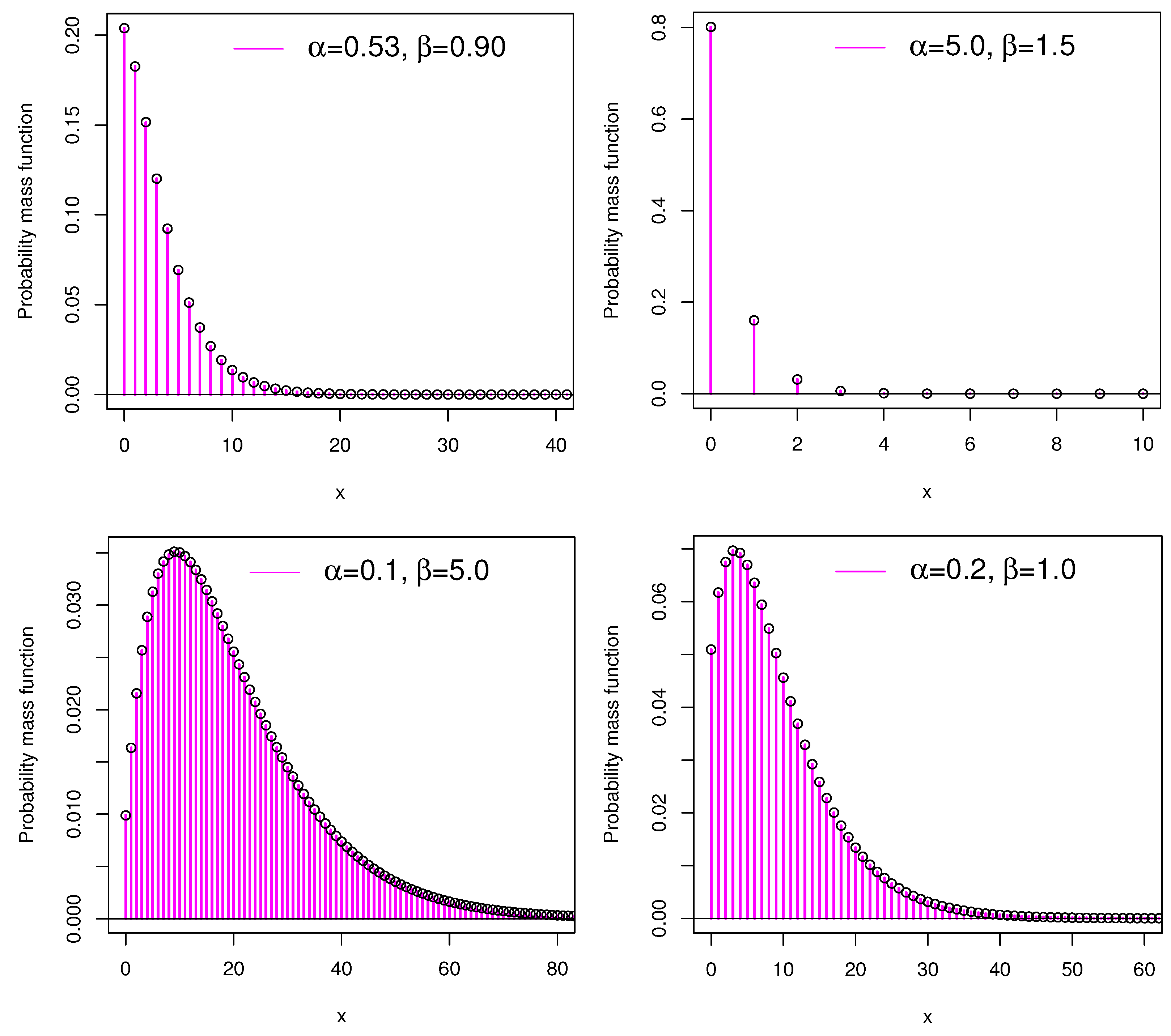
20], our applied work is more focused on the count regression model and the accompanying INAR(1) process, which are of current interest. Our theoretical work adds more aspects to the aforementioned study. Different pmf shapes are presented in Figure 1 for several parameter combinations of PEE distribution. The figure unequivocally demonstrates that the PEE distribution is right skewed.

2.1. Moments, Skewness and Kurtosis

Some results that can be derived from [20] are now presented in this portion. The probability-generating function for a random variable X with the PEE distribution is provided by
G ( s ; α , β ) = α 2 1 s + α + β ( α + β ) ( 1 + α s ) 2 ,
for | s | < α + 1 . Correspondingly, the moment-generating function of X is given by
M ( t ; α , β ) = α 2 1 e t + α + β ( α + β ) ( 1 + α e t ) 2 ,
for t log ( α + 1 ) . Let r be a positive integer. The rth factorial moment of a random variable X with the PEE distribution is given by
μ [ r ] = r ! α + β + β r α r ( α + β ) .
That is, in accordance with the definition of the rth factorial moment, we have μ [ r ] = 0 λ r α 2 ( 1 + β λ ) e α λ α + β d λ = α 2 α + β 0 λ r ( 1 + β λ ) e α λ d λ = Γ ( r + 1 ) α + β + β r α r ( α + β ) .
From the last equality, (5) is determined by applying the relation, Γ ( m + 1 ) = m ! , r being a positive integer. The first four non-central moments are derived as
E ( X ) = α + 2 β α ( α + β ) ,
E ( X 2 ) = α 2 + 6 β + 2 α ( 1 + β ) α 2 ( α + β ) ,
E ( X 3 ) = α 3 + 24 β + 2 α 2 ( 3 + β ) + 6 α ( 1 + 3 β ) α 3 ( α + β )
and
E ( X 4 ) = α 4 + 120 β + 2 α 3 ( 7 + β ) + 24 α ( 1 + 6 β ) + 6 α 2 ( 6 + 7 β ) α 4 ( α + β ) .
The variance of X is given by
V a r ( X ) = α 3 + α 2 + 4 α β + 3 α 2 β + 2 β 2 + 2 α β 2 α 2 ( α + β ) 2 .
The explicit versions of measures such as skewness and kurtosis of X can be found using the following formulas:
S ( X ) = E ( X 3 ) 3 E ( X 2 ) E ( X ) + 2 [ E ( X ) ] 3 [ V a r ( X ) ] 3 2
and
K ( X ) = E ( X 4 ) 4 E ( X 2 ) E ( X ) + 6 E ( X 2 ) [ E ( X ) ] 2 3 [ E ( X ) ] 4 [ V a r ( X ) ] 2 ,
respectively.

2.2. Dispersion Index and Coefficient of Variation

The dispersion index (DI) of the PEE distribution is given by
D I = V a r ( X ) E ( X ) = α 3 + 3 α 2 β + α 2 + 2 α β 2 + 4 α β + 2 β 2 α ( α + β ) ( α + 2 β ) .
As a complementary measure, the coefficient of variation (CV) of the PEE distribution is given by
C V = V a r ( X ) E ( X ) = α ( α + β ) α + 2 β α 3 + α 2 + 4 α β + 3 α 2 β + 2 β 2 + 2 α β 2 α ( α + β ) ( α + 2 β ) .
Now, Table 1 and Table 2 provide some numerical values for the PEE distribution’s mean, variance, and DI for a variety of parameter configurations. For the values considered, we check the mean, variance, and DI of the PEE distribution, and it is inferred that the DI of the PEE distribution is always greater than one, clearly showing overdispersion.

3. Parameter Estimation

3.1. Maximum Likelihood Estimation

Let X 1 , X 2 , . . . , X n be a random sample of size n from the PEE distribution with unknown parameters α and β , and x 1 , x 2 , . . . , x n be the related observations of the variables of this sample. Then the likelihood function is given by the following finite product:
L = i = 1 n α 2 ( 1 + α + β + β x i ) ( α + β ) ( α + 1 ) x i + 2 .
The maximum likelihood estimates (MLEs) of the parameters α and β , say α ^ and β ^ , are obtained by ( α ^ , β ^ ) = argmax ( α , β ) L or, in an equivalent manner in our setting, ( α ^ , β ^ ) = argmax ( α , β ) log L . To provide more practical facts, the normal equations are given by
log L α = 2 n α n α + β 2 n α + 1 + i = 1 n 1 1 + α + β + β x i i = 1 n x i α + 1
and
log L β = i = 1 n 1 + x i 1 + α + β + β x i n α + β .
Then α ^ and β ^ are obtained by solving the equation log L α = 0 and log L β = 0 , provided they reach a maximum well. This can only be achieved by a numerical optimization technique by using mathematical packages such as R, Mathematica and Python.

3.2. Simulation Study

The Monte Carlo simulation was performed to demonstrate the model’s efficiency using the maximum likelihood method. The estimates were calculated for true values of parameters for N = 1000 samples of sizes 50, 75, 200, 500, 750, and 1000. The following formulas are also used to calculate indices such as MLE, bias, mean square errors (MSEs), and coverage probabilities (CPs) and average lengths (ALs) of confidence intervals (CIs).
(i)
Mean value of MLEs: MLE ( h ^ ) = 1 N j = 1 N h ^ j .
(ii)
Average bias: Bias ( h ^ ) = 1 N j = 1 N ( h ^ j h ) .
(iii)
MSE: MSE ( h ^ ) = 1 N j = 1 N ( h ^ j h ) 2 .
(iv)
CP of CI: CP ( h ^ ) = 1 N j = 1 N I h ^ j 1.959964 × s j , h ^ < h < h ^ j + 1.959964 × s j , h ^ .
(v)
AL of CI: AL ( h ^ ) = 2 × 1.959964 N j = 1 N s j , h ^ .
Here, h = α or β , and s j , h ^ and I . denote the standard errors (SEs) of the MLEs and indicator function, respectively. Table 3 and Table 4 show the simulation results for two sets of parameter values. It has been found that MSEs and ALs of the CIs decrease with increasing sample size. The CPs of the CIs for each parameter are relatively close to the nominal 95 %  level.

4. PEE Regression Model

According to the previous section, the PEE model can model overdispersed data sets, which is critical since the majority of data in real life displays overdispersion. As a count regression model, this section uses the PEE distribution to model overdispersed data sets.

4.1. Model Construction

Let Y be a random variable representing the response variable and the number of occurrences of an event that follows the PEE distribution as well. To begin, let us consider the following reparametrization: β = α α 2 μ α μ 2 . With this configuration, we obtain the pmf of the PEE distribution in terms of the mean E ( Y ) = μ > 0 and α > 0 . Then the corresponding pmf is obtained as
P ( Y = y ; α , μ ) = α 2 1 + α + α α 2 μ α μ 2 + α α 2 μ α μ 2 y α + α α 2 μ α μ 2 ( α + 1 ) y + 2 ,
where y = 0 , 1 , 2 , . . . With the appropriate link functions, explanatory variables can be used to model the mean of the random variable Y. Covariates and the mean of the dependent variable can be linked using the log-link function. Let us consider Y 1 , Y 2 , . . . , Y n a random sample of size n from Y. Using the log-link function, the mean of Y i is linked to the covariate vector x i T = ( x i 1 , x i 2 , . . . , x i k ) T by the following equation:
μ i = E ( Y i ) = e x i T γ , i = 1 , 2 , , n ,
where γ = ( γ 0 , γ 1 , γ 2 , . . . , γ k ) is the unknown regression coefficients. Based on (7), a linear form for the pmf of Y i | X i T = x i T which follows the PEE distribution with parameter μ i , and α is obtained as
P ( y i ; α , e x i T γ ) = α 2 1 + α + α α 2 e x i T γ α e x i T γ 2 + α α 2 e x i T γ α e x i T γ 2 y i α + α α 2 e x i T γ α e x i T γ 2 ( α + 1 ) y i + 2 ,
where y i is the ith observations of Y.

4.2. Estimation of the Model

To estimate the regression coefficients γ , the maximum likelihood method is used. The logaritmic transformation of the likelihood function of the PEE count regression model is given by
log U = 2 n log α + i = 1 n log 1 + α + α α 2 e x i T γ α e x i T γ 2 + α α 2 e x i T γ α e x i T γ 2 y i i = 1 n log α + α α 2 e x i T γ α e x i T γ 2 log ( α + 1 ) i = 1 n y i + 2 .
Now the unknown parameter vector γ is obtained by maximizing (9). To accomplish this, we employ the optim function of R software. In addition, the SEs of these estimates are calculated using the fdHess function in R software.

4.3. Simulation of the PEE Regression Model

In this part, the maximum likelihood method used to estimate the unknown regression parameters is analysed using a simulation study. The parametric combinations ( α = 1.5 , γ 0 = 0.6 , γ 1 = 0.2 , γ 2 = 0.3 ) and ( α = 1.2 , γ 0 = 0.7 , γ 1 = 0.3 , γ 2 = 0.4 ) are used to generate N = 1000 samples of sizes n = 50, 100, 200, and 500 from the following model: log μ i = γ 0 + γ 1 x i 1 + γ 2 x i 2 . We assume that x i 1 and x i 2 are generated from the uniform distribution with parameters 0 and 1, which is denoted by U ( 0 , 1 ) . Here, indices such as estimates, bias, and MSEs are used to prove the asymptotic property of the MLEs. Table 5 reports the simulation results.
From Table 5, it is clear that as sample size increases, the bias and MSEs are decreasing, implying the consistency property of the MLEs for estimating the regression parameters.

5. INAR(1) Model with PEE Innovations

The INAR(1) process is widely used in the modeling of time series of counts in several scientific disciplines, including actuarial, finance, and medical. By applying the binomial thinning operator, INAR(1) differs from the first-order autoregressive process (AR(1)). The INAR(1) process is given by
X t = p X t 1 + ϵ t , t Z ,
where 0 p < 1 , and the innovation process is denoted by ϵ t t Z which are independent and identically distributed (iid) integer-valued random variables having mean, E ( ϵ t ) = μ ϵ and variance, V a r ( ϵ t ) = σ ϵ 2 . The binomial thinning operator is denoted by the symbol ∘ and is defined as
p X t 1 : = j = 1 X t 1 G j ,
where G j j 1 is the sequence of Bernoulli random variables with probability
p = P r ( G j = 1 ) = 1 P r ( G j = 0 ) .
For the INAR(1) process, the one-step transition probability matrix is given by
P r X t = k | X t 1 = l = i = 0 min ( k , l ) l i p i ( 1 p ) l i P r ( ϵ t = k i ) , k , l 0 ,
where 0 < p < 1 . There are many examples in real life where these types of stochastic processes play a role, including the number of passengers each year, the growth of bacteria each day, the number of scientific books cited, and many more. Here, a new INAR(1) process is introduced by assuming that the ϵ t innovations follow a PEE distribution. The one-step transition probability of the INAR(1)PEE model is given by
P r X t = k | X t 1 = l = i = 0 min ( k , l ) l i p i ( 1 p ) l i α 2 ( 1 + α + β + β ( k i ) ) ( α + β ) ( α + 1 ) ( k i ) + 2 .
So, hereafter, the described process will be called the INAR(1)PEE process.
Weiss C.H. [21] provide the mean, variance, and DI of X t t Z by using the mean, variance, and DI of the innovation distribution. For the INAR(1)PEE process, they are
E ( X t ) = α + 2 β α ( α + β ) ( 1 p ) ,
V a r ( X t ) = α 2 ( α + α p + 1 ) + 2 β 2 ( α + α p + 1 ) + α β ( 3 α ( p + 1 ) + 4 ) α 2 1 p 2 ( α + β ) 2
and
D I ( X t ) = 1 α + β 1 α + 2 β + 1 α + p + 1 1 p + 1 .
According to [21,22], the conditional expectation and variance of the INAR(1)PEE process are given by
E ( X t | X t 1 ) = p X t 1 + α + 2 β α ( α + β )
and
V a r ( X t | X t 1 ) = p ( 1 p ) X t 1 + α 3 + α 2 + 4 α β + 3 α 2 β + 2 β 2 + 2 α β 2 α 2 ( α + β ) 2 ,
respectively.

5.1. Estimation

The conditional maximum likelihod (CML), conditional least squares (CLS), and Yule–Walker (YW) methods are used to obtain the unknown parameters of the INAR(1) process.

5.1.1. Conditional Maximum Likelihood

The complicated form of the likelihood function resulting from the usual maximum likelihood method motivated the researchers to use the CML method instead of maximum likelihood. The knowledge of the transition probabilities is sufficient for the creation of likelihood in the CML technique since conditioning on the first observation results in a simple form of the likelihood, whereas there is no such conditioning present in the traditional maximum likelihood approach. The conditional log-likelihood function for the INAR(1)PEE process of the random sample X 1 , X 2 , . . . . , X T based on associated observations x 1 , x 2 , . . . , x T is given by
l ( p , α , β ) = log t = 2 T P r X t = x t | X t 1 = x t 1 = t = 2 T log P r X t = x t | X t 1 = x t 1 ,
where X 1 is fixed, and P r X t = x t | X t 1 = x t 1 is given by (13). By the maximization of (19), the CML estimates are obtained by using the constrOptim function of R.

5.1.2. Conditional Least Squares

The below function is minimized to obtain the CLS estimates of the parameters of the INAR(1) process
S ( p , α , β ) = t = 2 T x t E ( X t | X t 1 = x t 1 ) 2 .

5.1.3. Yule–Walker

As a result of the YW approach, the theoretical moments as well as the empirical ones are solved synchronously. Given that the autocorrelation function (ACF) of the INAR(1) process at lag η is ρ x ( η ) = p η , the YW estimate of p is given by
p ^ Y W = t = 2 T ( x t x ¯ ) ( x t 1 x ¯ ) t = 1 T ( x t x ¯ ) 2 ,
where x ¯ = 1 T t = 1 T x t . Now, the theoretical mean is solved with their empirical equivalents to derive the YW estimates of α and β . More precisely, when the theoretical mean equated with the empirical mean, we obtain
β ^ Y W = α ^ Y W α ^ Y W x ¯ ( 1 p ^ Y W ) 1 2 α ^ Y W x ¯ ( 1 p ^ Y W ) .
By substituting (21) in (16) and equating it with the sample dispersion, α ^ Y W is obtained.

5.2. Simulation

A simulation study was performed to check the finite sample performance of the CML, CLS, and YW estimates. In this regard, the number of replications is chosen as N = 1001 for different sample sizes, n = 50, 100, 200, 300, and 500. The two parameter vectors used here are ( p = 0.5 , α = 0.7 , β = 1 ) and ( p = 0.7 , α = 0.5 , β = 0.8 ). The simulation results are interpreted based on the biases and MSEs. The R-code is given in Appendix A. Table 6 and Table 7 show the results. The biases and MSEs of the CML estimates are the smallest when the three estimation methods are compared, and the CML estimation approach outperforms the others. The CML estimation approach is then applied.

6. Empirical Studies

With the help of three real-life data sets, the superiority of the PEE model is illustrated.

6.1. Corn Borer Data

The first data set is from [23]. The data are from the biological experiment, representing the number of larvae of the European corn borer (ECB) in the field (Pyrausta).
Several competing distributions were compared to the fit of the PEE distribution, including the discrete Burr (DB) distribution (see [24]), the discrete log-logistic (DLL) distribution (see [25]), the discrete Gumbel (DG) distribution (see [26]), the Poisson quasi-xgamma (PQX) distribution (see [13]), the exponentiated discrete Lindley (EDL) distribution (see [27]), the discrete Bilal (DBL) distribution (see [28]), the discrete inverse Rayleigh (DIR) distribution, and the discrete Pareto (DP) distribution (see [24]).
Utilizing the optim function of R, the Hessian and the Fisher information matrices are assessed. Each parameter’s SE is evaluated by using the fact that the SEs can be computed as the square root of the diagonal elements of the inverse of the Fisher information matrix. As shown in Table 8, the MLEs with their corresponding SEs and confidence intervals (CIs) (lower bound of CI, upper bound of CI) for the numbers of borers data set are provided. From Table 9, it is clearly evident that the PEE distribution is the best among the considered competitive models since it has the lowest AIC, BIC, and value with the highest log L and p-value. The fitted PEE distribution is overdispersed since the mean and variance of the PEE distribution for the corn borer data are 1.375 and 2.2131, respectively.
Figure 2 presents the estimated pmfs of all the considered models from which the distribution adequacy of the PEE model is clearly seen.

6.2. Length of Hospital Stay

The effectiveness of the count regression model under the PEE distribution is assessed using the second data set. The data consists of 3589 observations from the files of 1991 Arizona cardiovascular patients that were located in the COUNT package of the R programming language. The PEE regression model is used to model the length of stay ( y i ) by using the covariates: cardiovascular procedure ( x 1 i ) (1 = CABG, 0 = PTCA), sex ( x 2 i ) (1 = male, 0 = female), type of admission ( x 3 i ) (1 = urgent, 0 = elective), and age ( x 4 i ) (1 = age > 75, 0 = age ≤ 75). Given below is the regression structure which will be fitted by the PEE distribution, the new Poisson generalized Lindley (NPGL) regression model (see [29]), the Poisson-xgamma (PX) regression model (see [7]), the Poisson–Lindley (PL) regression model and the basic Poisson regression model:
μ i = e γ 0 + γ 1 x 1 i + γ 2 x 2 i + γ 3 x 3 i + γ 4 x 4 i .
The mean and variance of the dependent variable are calculated as 8.831 and 47.973, respectively, stating the clear overdispersion. Table 10 gives the parameter estimates and results of information criterion.
Altun E. [29] used this data set to prove the better fit of the NPGL regression model. Hence, from Table 10, it is clear that the PEE regression model is better than competing models since it has minimized values for its -log L, AIC, and BIC. We thus conclude that it will be a more appropriate model than the other models for modelling this data set. As a result, we can say that the length of hospital stay increases when people have CABG cardiovascular surgery, are admitted urgently, and are over the age of 75. Additionally, female individuals have a longer hospital stay than male individuals.

6.3. Weekly Number of Syphilis Cases Data

Here, the performance of the INAR(1)PEE process is carried out with other famous INAR(1) processes such as the INAR(1)P process (see [10]), the INAR(1)G process (see [12]), the INAR(1)PTE process (see [30]), and the INAR(1)PWE process (see [5]). The data set used here is the weekly number of syphilis cases in the United States from 2007 to 2010 in New York. The ZIM package of the R software contains the data. The mean, variance, and DI of the data set are 24.6316, 105.6761, and 4.2903, respectively. The data have statistically significant overdispersion according to the test [31] presented, which results in a p-value of less than 0.001. In Figure 3, the fundamental plots of the data set, including the ACF, the partial ACF (PACF), the histogram, and the time series plots, are depicted. It is concluded that the INAR(1) process could be a possible model for this data set, since only the first lag is significant in the PACF plot. As shown in Table 11, fitting INAR(1) processes with the PEE innovations and other corresponding innovations yields parameter estimates along with SE, AIC, BIC, theoretical mean, variance, and DI. The minimum AIC and BIC statistics values for the INAR(1)PEE process demonstrate that it offers a better fit than other INAR(1) processes. The theoretical DI value for the INAR(1)PEE process is also relatively close to the empirical one. In light of this, it is believed that the INAR(1)PEE process provides a very good explanation for the properties of the data set.

7. Conclusions

7.1. Concluding Remarks

This paper focuses on a two-parameter discrete distribution obtained by compounding the Poisson and EE distributions and called the PEE distribution. The properties of the PEE distribution were derived and discussed. The properties, including the factorial moments, the moment-generating function, and the probability-generating functions, are evaluated, and they are in explicit forms. The article thus highlights the PEE distribution and, for the first time, its regression model and the INAR(1) model. The PEE model is found to outperform all other compared models in all aspects of the present study. In the modelling of positive integer-valued data sets from various fields of study, the proposed model is expected to increase its prevalence and have a broader variety of applications.

7.2. Future Work

This study may take a different turn if either the bivariate PEE model and its corresponding BINAR(1) model or the pth-order integer-valued auto regressive process (INAR(p)) with PEE innovations are developed. We will leave the substantial revisions, research, and software support for this effort to future studies.

Author Contributions

Conceptualization, R.M., C.C., A.K. and M.R.I.; methodology, R.M., C.C., A.K. and M.R.I.; software, R.M., C.C., A.K. and M.R.I.; validation, R.M., C.C., A.K. and M.R.I.; formal analysis, R.M., C.C., A.K. and M.R.I.; investigation, R.M., C.C., A.K. and M.R.I.; resources, R.M., C.C., A.K. and M.R.I.; data curation, R.M., C.C., A.K. and M.R.I.; writing—original draft preparation, R.M., C.C., A.K. and M.R.I.; writing—review and editing, R.M., C.C., A.K. and M.R.I.; visualization, R.M., C.C., A.K. and M.R.I. All authors have read and agreed to the published version of the manuscript.

Funding

This research received no external funding.

Institutional Review Board Statement

Not applicable.

Informed Consent Statement

Not applicable.

Data Availability Statement

Not applicable.

Acknowledgments

The authors would also like to thank three reviewers for their thorough comments which led to improvement in the presentation of the manuscript.

Conflicts of Interest

The authors declare no conflict of interest.

Appendix A

R-code for the generation of random numbers from the INAR(1)PEE process.
library(nleqslv)
datt=NULL
ppois=function(x,alpha,theta){
f=1-(((alpha+1)^(-(x+2))*(alpha+alpha^2+theta+(x+2)*alpha*theta))
/(alpha+theta))
return(f)
ppois(2,0.5,1)
r.pois <- function(n, L,T)
{
U <- runif(n)
X <- rep(0,n)
for(i in 1:n)
{
if(U[i] < ppois(0,L,T))
{
X[i] <- 0
} else
{B = FALSE
I = 0
while(B == FALSE)
{int <- c( ppois(I, L,T), ppois(I+1,L,T) )
if( (U[i] > int[1]) & (U[i] < int[2]) )
{X[i] <- I+1
B = TRUE
} else
{I=I+1
}}}}
return(X)
}
r.pois(50, 1.5, 1.2)
r.inarnpl=function (n, alpha, lambda,theta, n.start = NA)
{length. <- n + n.start
x <- rep(NA, times = length.)
error <- r.pois(length., lambda,theta)
x[1] <- error[1]
for (t in (2):length.) {
x[t] <- 0
for (j in 1:1) {
x[t] <- x[t] + rbinom(1, x[t - 1], alpha)
}
x[t] <- x[t] + error[t]
}
ts(x[(n.start + 1):length.], frequency = 1, start = 1)
}
(x <- as.numeric(r.inarnpl(100, 0.5, 0.5, 0.2, 200)))

References

  1. Bereta, E.M.; Louzada, F.; Franco, M.A. The Poisson-Weibull distribution. Adv. Appl. Stat. 2011, 22, 107–118. [Google Scholar]
  2. Bhati, D.; Kumawat, P.; Gómez-Déniz, E. A new count model generated from mixed Poisson transmuted exponential family with an application to health care data. Commun. Stat.—Theory Methods 2017, 46, 11060–11076. [Google Scholar] [CrossRef]
  3. Mahmoudi, E.; Zakerzadeh, H. Generalized Poisson–Lindley distribution. Commun. Stat. —Theory Methods 2010, 39, 1785–1798. [Google Scholar] [CrossRef]
  4. Miao, Y.; Kook, J.H.; Lu, Y.; Guindani, M.; Vannucci, M. Scalable Bayesian variable selection regression models for count data. In Flexible Bayesian Regression Modelling; Academic Press: Cambridge, MA, USA, 2020; pp. 187–219. [Google Scholar]
  5. Altun, E. A new generalization of geometric distribution with properties and applications. Commun. Stat.—Simul. Comput. 2020, 49, 793–807. [Google Scholar] [CrossRef]
  6. Altun, E. A new one-parameter discrete distribution with associated regression and integer-valued autoregressive models. Math. Slovaca 2020, 70, 979–994. [Google Scholar] [CrossRef]
  7. Altun, E.; Cordeiro, G.M.; Ristic, M.M. An one-parameter compounding discrete distribution. J. Appl. Stat. 2022, 49, 1935–1956. [Google Scholar] [CrossRef]
  8. Wongrin, W.; Bodhisuwan, W. Generalized Poisson–Lindley linear model for count data. J. Appl. Stat. 2017, 44, 2659–2671. [Google Scholar] [CrossRef]
  9. Al-Osh, M.A.; Alzaid, A.A. First-order integer-valued autoregressive (INAR(1)) process. J. Time Ser. Anal. 1987, 8, 261–275. [Google Scholar] [CrossRef]
  10. McKenzie, E. Some simple models for discrete variate time series 1. JAWRA J. Am. Water Resour. Assoc. 1985, 21, 645–650. [Google Scholar] [CrossRef]
  11. McKenzie, E. Autoregressive moving-average processes with negative-binomial and geometric marginal distributions. Adv. Appl. Probab. 1986, 18, 679–705. [Google Scholar] [CrossRef]
  12. Aghababaei Jazi, M.; Jones, G.; Lai, C.D. Integer valued AR(1) with geometric innovations. J. Iran. Stat. Soc. 2012, 11, 173–190. [Google Scholar]
  13. Altun, E.; Bhati, D.; Khan, N.M. A new approach to model the counts of earthquakes: INARPQX(1) process. SN Appl. Sci. 2021, 3, 1–17. [Google Scholar] [CrossRef]
  14. Gómez, Y.M.; Bolfarine, H.; Gómez, H.W. A new extension of the exponential distribution. Rev. Colomb. Estad. 2014, 37, 25–34. [Google Scholar] [CrossRef] [Green Version]
  15. Shanker, R.; Sharma, S.; Shanker, R. A two-parameter Lindley distribution for modeling waiting and survival times data. Appl. Math. 2013, 4, 363–368. [Google Scholar] [CrossRef] [Green Version]
  16. Gómez, Y.M.; Gallardo, D.I.; Leao, J.; Gómez, H.W. Extended exponential regression model: Diagnostics and application to mineral data. Symmetry 2020, 12, 2042. [Google Scholar] [CrossRef]
  17. de Andrade, T.A.; Bourguignon, M.; Cordeiro, G.M. The exponentiated generalized extended exponential distribution. J. Data Sci. 2016, 14, 393–413. [Google Scholar] [CrossRef]
  18. Rasekhi, M.; Alizadeh, M.; Altun, E.; Hamedani, G.G.; Afify, A.Z.; Ahmad, M. The modified exponential distribution with applications. Pak. J. Stat. 2017, 33, 383–398. [Google Scholar]
  19. Rasekhi, M.; Chatrabgoun, O.; Daneshkhah, A. Discrete weighted exponential distribution: Properties and applications. Filomat 2018, 32, 3043–3056. [Google Scholar] [CrossRef]
  20. Shanker, R.; Sharma, S.; Shanker, R. A discrete two-parameter Poisson Lindley distribution. J. Ethiop. Stat. Assoc. 2012, 21, 15–22. [Google Scholar]
  21. Weiss, C.H. An Introduction to Discrete-Valued Time Series; John Wiley & Sons: Hoboken, NJ, USA, 2018. [Google Scholar]
  22. Al-Osh, M.; Alzaid, A.A. Integer-valued moving average (INMA) process. Stat. Pap. 1988, 29, 281–300. [Google Scholar] [CrossRef]
  23. Bodhisuwan, W.; Sangpoom, S. The discrete weighted Lindley distribution. In Proceedings of the 2016 12th International Conference on Mathematics, Statistics, and Their Applications (ICMSA), Banda Aceh, Indonesia, 4–6 October 2016; pp. 99–103. [Google Scholar]
  24. Krishna, H.; Pundir, P.S. Discrete Burr and discrete Pareto distributions. Stat. Methodol. 2009, 6, 177–188. [Google Scholar] [CrossRef]
  25. Para, B.A.; Jan, T.R. Discrete version of log-logistic distribution and its applications in genetics. Int. J. Mod. Math. Sci. 2016, 14, 407–422. [Google Scholar]
  26. Chakraborty, S.; Chakravarty, D. A discrete Gumbel distribution. arXiv 2014, arXiv:1410.7568. [Google Scholar]
  27. El-Morshedy, M.; Eliwa, M.S.; Nagy, H. A new two-parameter exponentiated discrete Lindley distribution: Properties, estimation and applications. J. Appl. Stat. 2020, 47, 354–375. [Google Scholar] [CrossRef]
  28. Altun, E.; El-Morshedy, M.; Eliwa, M.S. A study on discrete Bilal distribution with properties and applications on integer-valued autoregressive process. RevStat Stat. J. 2020, 18, 70–99. [Google Scholar]
  29. Altun, E. A new two-parameter discrete poisson-generalized Lindley distribution with properties and applications to healthcare data sets. Comput. Stat. 2021, 36, 2841–2861. [Google Scholar] [CrossRef]
  30. Altun, E.; Khan, N.M. Modelling with the novel INAR(1)-PTE process. Methodol. Comput. Appl. Probab. 2022, 24, 1735–1751. [Google Scholar] [CrossRef]
  31. Schweer, S.; Weiß, C.H. Compound Poisson INAR (1) processes: Stochastic properties and testing for overdispersion. Comput. Stat. Data Anal. 2014, 77, 267–284. [Google Scholar] [CrossRef]
Figure 1. Various shapes of the pmfs of the PEE distribution for the varying values of the parameters.
Stats 05 00044 g001
Figure 2. Pmfs of fitted models for corn borer data.
Stats 05 00044 g002
Figure 3. ACF, PACF, time series, and histogram plots of weekly number of syphilis cases data.
Stats 05 00044 g003
Table 1. Moment measure values for the PEE distribution for α = 0.5 and various β values.
Measures β
0.10.50.92.658
Mean2.33333.03.28573.67743.81823.8824
Variance7.555610.010.775511.573411.785111.8685
DI3.23813.33333.27953.14713.08663.0570
Table 2. Moment measure values for the PEE distribution for β = 1.5 and various α values.
Measures α
0.10.95.09.011.0
Mean19.37501.80560.24620.12700.1018
Variance218.98444.10110.30250.14260.1119
DI11.30242.27141.22881.12301.0995
Table 3. Simulation results for α = 0.5 and β = 0.9 .
α = 0.5 , β = 0.9
Parameter n MLEBiasMSECPAL
α 500.4839−0.01610.00900.99700.5243
750.4867−0.01330.00710.99200.4322
2000.4894−0.01060.00320.99100.2640
5000.4974−0.00260.00130.97900.1560
7500.4996−0.00040.00090.97200.1274
10000.4997−0.00030.00070.97700.1103
β 500.96050.06050.32200.87905.3376
750.95480.05480.29330.88404.6352
2000.94780.04780.21340.90603.0661
5000.94050.04050.14750.92202.0805
7500.92970.02970.12150.93101.7183
10000.92080.02080.09780.93801.4755
Table 4. Simulation results for α = 1.2 and β = 0.8 .
α = 1.2 , β = 0.8
Parameter n MLEBiasMSECPAL
α 501.1537−0.04630.08320.99502.4724
751.1704−0.02960.06540.98501.9964
2001.1707−0.02930.04320.99401.4188
5001.1739−0.02610.02820.98400.9127
7501.1806−0.01940.02220.99200.7404
10001.1815−0.01850.01850.99400.6468
β 500.87030.07030.45690.89508.5865
750.86410.06410.45540.87707.3207
2000.85240.05240.38430.87704.9990
5000.84560.04560.30890.92203.5077
7500.84070.04070.26110.94402.8943
10000.82130.02130.23650.95702.5458
Table 5. Simulation results for the PEE regression model.
α = 1.5 , γ 0 = 0.6 , γ 1 = 0.2 , γ 2 = 0.3 α = 1.2 , γ 0 = 0.7 , γ 1 = 0.3 , γ 2 = 0.4
n ParametersEstimatesBiasMSE n ParametersEstimatesBiasMSE
50 α 0.69630.80370.645950 α 0.65220.54780.3001
γ 0 0.42240.17760.7988 γ 0 0.51560.18441.1900
γ 1 0.17450.02550.2899 γ 1 0.33290.03290.5317
γ 2 0.14060.15940.2775 γ 2 0.15780.24220.3585
100 α 0.72890.77110.5946100 α 0.67320.52680.2775
γ 0 0.50770.09230.7280 γ 0 0.78760.08761.0121
γ 1 0.21170.01170.2397 γ 1 0.27110.02890.3790
γ 2 0.15600.14400.2486 γ 2 0.16370.23630.2430
200 α 0.78570.71430.5103200 α 0.71350.48650.2367
γ 0 0.66450.06450.5838 γ 0 0.62430.07570.8479
γ 1 0.20740.00740.2277 γ 1 0.32170.02170.3546
γ 2 0.17100.12900.2241 γ 2 0.18520.21480.2408
500 α 0.80310.69690.4856500 α 0.72010.47990.2303
γ 0 0.60190.00190.5448 γ 0 0.72730.02730.7893
γ 1 0.20580.00580.2093 γ 1 0.31710.01710.3164
γ 2 0.17120.12880.1559 γ 2 0.19630.20370.2028
Table 6. Simulation for the INAR(1)PEE model for p = 0.5 , α = 0.7 and β = 1 .
p = 0.5 , α = 0.7 , β = 1
Parameter n CMLCLSYW
BiasMSEBiasMSEBiasMSE
p500.00410.0048−0.05180.0197−0.06140.0204
1000.00200.0024−0.02580.0088−0.03070.0089
2000.00130.0014−0.01410.0047−0.01640.0048
3000.00100.0008−0.00620.0027−0.00770.0028
5000.00090.0006−0.00460.0018−0.00570.0018
α 50−0.03180.0233−0.01100.0237−0.43070.1912
100−0.03120.0159−0.00780.0121−0.41520.1762
200−0.02800.0115−0.00440.0063−0.39690.1605
300−0.01910.00880.00260.0040−0.38650.1523
500−0.01280.00550.00160.0025−0.38230.1482
β 50−0.03360.37160.09690.0677−0.93610.8767
100−0.02440.36490.08250.0422−0.93600.8766
200−0.02150.33030.06750.0251−0.93570.8756
300−0.00530.30240.05200.0149−0.93520.8746
500−0.00210.25140.05140.0111−0.93470.8737
Table 7. Simulation for the INAR(1)PEE model for p = 0.7 , α = 0.5 , β = 0.8 .
p = 0.7 , α = 0.5 , β = 0.8
Parameter n CMLCLSYW
BiasMSEBiasMSEBiasMSE
p500.00070.0018−0.06010.0182−0.07510.0200
1000.00060.0010−0.03470.0071−0.04180.0076
2000.00040.0005−0.01680.0032−0.02060.0033
3000.00020.0003−0.00950.0018−0.01210.0018
5000.00010.0002−0.00560.0011−0.00700.0011
α 50−0.02140.0122−0.02700.0209−0.33350.1144
100−0.02020.0081−0.02140.0105−0.31590.1021
200−0.01700.0053−0.00890.0055−0.30080.0923
300−0.01140.0039−0.00200.0032−0.29000.0855
500−0.01130.0024−0.00100.0020−0.28230.0810
β 500.13020.44550.10810.0866−0.76030.5782
1000.12000.39120.07850.0368−0.75740.5738
2000.11430.35440.06440.0209−0.75540.5707
3000.10920.31450.05350.0140−0.75450.5694
5000.08180.25970.05310.0168−0.75440.5692
Table 8. Corn borer data: MLEs, SEs and CIs.
StatisticPEEDBDLLDGPQXEDLDBLDIRDP
MLE α 1.05832.35701.94293.10630.92590.46910.65660.31960.3292
SE α 0.27510.36550.18790.36670.87180.04210.01860.04210.0338
95% CIlower α 0.51901.64071.57452.387600.38650.62020.23700.2630
upper α 1.59763.07332.31133.82502.63460.55170.69300.40220.3954
MLE β 1.40220.51901.40070.40671.37430.9015---
SE β 2.48930.05080.12120.02940.33910.1707---
95% CIlower β 00.41941.16310.34920.70970.5669---
upper β 6.28120.61861.63830.46422.03891.2361---
Table 9. Corn borer data: MLE, χ 2 , p-value, AIC and BIC for the competitive models.
XOfPEEDBDLLDGPQXEDLDBLDIRDP
04344.616743.835941.031728.553345.476544.024432.733738.352064.4467
13530.459839.600638.938137.861129.332030.590539.585651.874320.1489
21719.065815.621817.775225.584818.784319.456524.277215.48909.6863
31111.33617.20638.431512.852011.522611.565012.50776.02755.6474
456.51473.91024.48465.70016.75426.58455.97022.90503.6805
543.65452.37552.63002.40173.80563.63862.73751.60962.5800
612.01321.56251.66340.99092.07501.96681.22650.98141.9042
721.09361.08941.11520.40541.10121.04520.54190.64141.4605
821.24564.79773.93045.65061.14871.12860.41982.119810.4456
Total120120120120120120120120120120
log L−200.4152−204.2933−202.6303−213.1911−200.6567−200.4922−204.6753−208.4404−220.6182
AIC404.8303412.5865409.2606430.3823405.3134404.9844411.3505418.8808443.2363
BIC410.4053418.1615414.8356435.9573410.8883410.5593414.1380421.6683446.0238
χ 2 0.98772.67391.31137.61511.47601.00706.996114.294930.5180
df222222333
p-value0.61030.26260.51910.02220.47810.60440.07200.00250.0001
Table 10. The MLE, −log L, AIC and BIC of the fitted regression models for the length of stay data set.
CovariatesPPLPQXNPGLPEE
Estimate SEp-ValueEstimate SEp-ValueEstimate SEp-ValueEstimate SEp-ValueEstimate SEp-Value
γ 0 1.4560<0.0011.4133<0.0011.3996<0.0011.4044<0.0011.3968<0.001
0.01580.03720.03490.03530.0345
γ 1 0.9606<0.0010.9843<0.0010.9725<0.0010.9761<0.0010.9932<0.001
0.01220.02910.02700.02740.0271
γ 2 −0.1240<0.001−0.1288<0.001−0.1269<0.001−0.1267<0.001−0.1276<0.001
0.01180.03040.02800.02850.0284
γ 3 0.3266<0.0010.3843<0.0010.3732<0.0010.3759<0.0010.3938<0.001
0.01210.03020.02800.02840.0281
γ 4 0.1224<0.0010.1193<0.0010.1202<0.0010.1198<0.0010.1197<0.001
0.01240.03230.02980.03030.0302
−log L−11,189.8976−10,625.5957−10,569.8162−10,563.2551−10,428.6400
AIC22,389.795221,239.191321,127.632421,114.510220,845.2700
BIC22,420.723321,202.077521,090.518721,077.396420,808.1600
Table 11. Estimates and modelling adequacy statistics for the number of syphilis cases data.
ModelParametersEstimateSt. ErrorAICBIC μ x σ x 2 DI x
INAR(1)PEE α 0.10500.00741629.88481639.911823.0431144.35876.2647
β 5.50007.5600
p0.23650.0371
INAR(1)P λ 21.06340.70872016.53952023.224225.349325.34931
p0.14800.0261
INAR(1)G λ 0.05830.00471686.42771693.112423.8947252.431210.5643
p0.34690.0323
INAR(1)PWE λ 0.05840.15891688.42771698.454724.9904369.211414.7741
α 0.05982.8834
p0.34680.0323
INAR(1)PTE λ −1.00000.08601637.05441647.081425.2105278.426611.0441
α 0.07880.0058
p0.24250.0390
Empirical 24.6316105.67614.2903
Publisher’s Note: MDPI stays neutral with regard to jurisdictional claims in published maps and institutional affiliations.

