Combined Control System for the Coordinates of the Electric Mode in the Electrotechnological Complex “Arc Steel Furnace-Power-Supply Network”

Abstract

To stabilize the electrical mode of an arc steelmaking furnace in the initial stages of melting, it is advisable to use a high-speed current-limiting system, in addition to the traditional electrode movement control system. This system is implemented by including the primary winding of the furnace transformer choke, controlled by thyristors. The use of such a system, on the one hand, reduces the negative impact of the arc steel furnace on the the power supply network operation and, on the other, affects the operation of the electrode movement system, built on the principle of an impedance regulator. In order to analyze the mutual influences between such systems, a mathematical model for the power supply and control system of the arc steelmaking furnace was created. The developed model can work in real time, which corresponds to the world trends of modern control system synthesis for complex technological objects. In the created model, the work of the combined control system with different approaches to the formation of the control effect in the high-speed circuit and the effect of the combined control system on the power supply system of the ASF are analyzed.

1. Introduction

Steel is one of the main pillars of modern society and, as one of the most important engineering and construction materials, affects the work of most industries. According to the International Energy Agency (IEA), global demand for steel will increase by more than a third by 2050 [1]. Although steel is one of the most recyclable materials on the planet, the energy needs for initial production make it one of the largest consumers of coal. The metallurgical industry consumes about 7% of the produced energy and, according to conservative estimates, it accounts for 7–9% of global greenhouse gas emissions. According to IEA reports, in order to achieve the global energy and climate goals, emissions from the steel industry must be reduced by at least 50% up to 2050. One of the ways to achieve such ambitious goals is the development of electrometallurgy.

Today, about a third of the world’s steel is produced by the electric arc method, which uses high-current electric arcs to melt scrap steel. The availability of green electricity, changes in the emissions trading system (ETS) and the development of new technologies provide the opportunity to significantly increase the share of steel smelting in arc steelmaking furnaces in the coming decades [2,3]. Currently, modern ASFs for smelting 1 ton of steel consume approximately 330 kWh of electricity [1]. A 300-ton ASF with a capacity of 300 MVA coexists in the melting process (proceed about 37 min) approximately 132 MWh of energy. Thus, even a small increase in energy efficiency can provide significant savings.

The problem of reducing electricity costs for smelting one ton of steel encourages leading electrical companies to create and implement new control systems for ASFs. However, the dynamic asymmetric and stochastic nature of the ASF load and the presence of significant nonlinearities in the power supply circuit of a three-phase arc system and in the automatic electric control system make ASFs one of the most complex technological objects in terms of automation and implementation of optimal control modes. Today, we know the technological solutions of such leading companies as Siemens (SIMETAL system), Danieli (HI-REG and Q-REG + systems) and others, which provide optimal control of the movement of the arc electrode based on certain factors. The purpose of adjusting the arc length is to implement the desired voltage–current control for a given voltage converter. The most common control strategies are based on the impedance control principle, control by deviation from the specified value of voltage or current [4,5,6,7]. The choice of strategy usually takes into account various factors, in particular: the required active power during the melting period, the melting process, the technical capabilities of the equipment, etc. The most widespread architecture of the electrode movement control system in an AFS is the MISO structure (several inputs, single output), which, as a rule, implements independent control of each phase. The use of adaptive control or intelligent control technologies in such a structure makes it possible to improve the quality of control compared to the system synthesized on the basis of classical control theory [8,9,10,11,12,13]. However, from an electrical point of view, the phases are interdependent, which causes unproductive movements in the electrodes and, thus, impairs the quality of control.

The use of the control structure type MIMO (multiple inputs, multiple outputs) can improve the quality of control [14]. The synthesis of control effects in such a control system requires the use of a system model that allows one to take into account the mutual influences between the phases. The complexity of applying classical control theory for the MIMO controller synthesis using adequate models of such a complex object as AFS [15,16,17] has contributed to the widespread use of artificial neural network theory to solve the problem of control effect formation [18,19,20,21].

However, the control system of electrode movement due to significant inertia is unable to compensate for the negative effects on the power supply network caused by changes in the situation in the arc space. In particular, with a short circuit, the active power becomes almost zero, while the reactive power increases sharply. Thus, the initial period of melting is characterized by significant and rapid changes in active and reactive power with high peaks for the latter; significant in amplitude and very fast changes in current, in particular high values of reactive current; and rapid changes in the power factor [22]. Changing the situation in the furnace space (occurrence of single-phase or two-phase short circuits, arc breakage, etc.) and nonlinearity of the volt-ampere characteristic of the arc cause asymmetric modes and higher harmonic components in the power supply [23,24,25], which significantly, highlights the problem of electromagnetic compatibility in the arc steel furnace and the power supply system.

In ASFs, the power supply system traditionally consists of a furnace transformer with taps on the secondary winding and, sometimes, a reactor connected in series with the primary winding of the transformer. As shown in [26,27,28,29], the use of a controlled reactor allows you to effectively limit the current value, minimize the load asymmetry coefficient on the phases in the arc furnace and improves the power factor, increasing the productivity of the furnace. In [30], the optimal reactor control from the point of view of complex system approach is analyzed, in which the arc steelmaking furnace and power supply network are considered as the only complex electrotechnological system, the control vector of which is synthesized. As noted in [31], such control can be implemented and a significant effect can be obtained only in the hierarchical structures of systems of extreme adaptive (situational) control and high-speed control of the coordinates in the electric mode. At the same time, the synthesis and implementation of optimal control in terms of increasing the productivity of the furnace and reducing the specific cost of electricity is a many-times-more-effective approach than developing solutions for high-quality stabilization of the coordinates in the ER.

The current trend of automation for technological processes is the creation of intelligent industries with the widespread use of “digital duplicates” [32,33,34] and mathematical models capable of working in real time [35,36,37,38,39]. Due to the continuous melting change in stochastic characteristics of perturbations in the melting space and power circuit of the furnace, the need to change the parameters of electricity flow during changes in physicochemical state and temperature regimes of charge and melt, using a systematic approach to control electrotechnological complex “ASF- power supply system”, it is advisable to use a mathematical model that can work in real time. This will make it possible to apply model predictive control technology and evaluate the effectiveness of control effects in the melting process, taking into account the interaction of the high-speed control circuit and the electrode movement of the arc steelmaking furnace.

Thus, the synthesis of a mathematical model that describes electromagnetic processes in the power supply system of an arc steel furnace and makes it possible to synthesize and analyze the effectiveness of control influences, taking into account the mutual action of all subsystems, is an actual task, the solution of which is proposed in this article.

2. Mathematical Model of the Power Circuit and Calculation Algorithm

In such a case, the model for studying the influence of EAF on the power supply network should contain a model of the electric circuit with controlled reactor, taking into account the nonlinearity of the volt-ampere characteristic of the arc, the model of the control system of EAF electrode movement and the model of random arc length processes. EAF with a controlled reactor contains different tempo subsystems and is characterized by a significant range of changes in electrical regime parameters in the melting modes (in particular, due to changes in the dynamic resistance of the arc and control influences in subsystems). The proposed model provides a possibility to analyze the effectivity of the controlled influences in traditional (electrode moving) and high-speed (controlled reactor) control systems, taking into account the mutual influence of both systems and electromagnetic processes in different phases of an EAF electric power supply.

2.1. Basic Principles of Mathematical Modeling Solution Algorithm

A mathematical model for the power circuit of the system “arc steelmaking furnace—power supply system” and its computer application was created using an object-oriented method [40,41], according to which the model is formed from typical elements presented in the form of multipoles. This method was used in [17], to create a real-time model of the electrical complex with AFS. In the framework of this study, the mathematical model proposed in [17] was supplemented by an adjustable reactor (magneto-thyristor voltage regulator MTVR). The corresponding calculation scheme of the model is shown in Figure 1.

The scheme is formed by connecting the outer circuits of multipole elements, namely: three-phase network, controlled reactor (represented by a combination of thyristor voltage regulator and three-phase inductor), transformer and three-phase short circuit with an arc. The outer circuits of these multipolar elements are interconnected at the nodes of the system. The potentials of the independent nodes of the system are denoted as ν₁–ν₉.

According to the theory of multipoles, the method of connecting a multipole element is described by an incidence matrix containing 0 and 1 and indicating which independent node in the system is connected to the pole of the element. Let us denote the incident matrices: Π_N (three phases power supply), Π_TVR (thyristor voltage regulator), Π_r (three-phase choke), Π_TR (transformer) and Πa Π_SL (three-phase short connection with an arc). Such matrices will be used for equations on electrical potential in system nodes.

According to the calculation scheme in Figure 1, these matrices will appear as:

$$\begin{gathered} {\Pi }_N=\left[\begin{array}{cccccc}0& 0& 0& 1& 0& 0\\ 0& 0& 0& 0& 1& 0\\ 0& 0& 0& 0& 0& 1\\ 0& 0& 0& 0& 0& 0\\ 0& 0& 0& 0& 0& 0\\ 0& 0& 0& 0& 0& 0\\ 0& 0& 0& 0& 0& 0\\ 0& 0& 0& 0& 0& 0\\ 0& 0& 0& 0& 0& 0\end{array}\right],{\Pi }_{TVR}={\Pi }_r=\left[\begin{array}{cccccc}1& 0& 0& 0& 0& 0\\ 0& 1& 0& 0& 0& 0\\ 0& 0& 1& 0& 0& 0\\ 0& 0& 0& 1& 0& 0\\ 0& 0& 0& 0& 1& 0\\ 0& 0& 0& 0& 0& 1\\ 0& 0& 0& 0& 0& 0\\ 0& 0& 0& 0& 0& 0\\ 0& 0& 0& 0& 0& 0\end{array}\right],{\Pi }_r=\left[\begin{array}{cccccc}0& 0& 0& 1& 0& 0\\ 0& 0& 0& 0& 1& 0\\ 0& 0& 0& 0& 0& 1\\ 0& 0& 0& 0& 0& 0\\ 0& 0& 0& 0& 0& 0\\ 0& 0& 0& 0& 0& 0\\ 0& 0& 0& 0& 0& 0\\ 0& 0& 0& 0& 0& 0\\ 0& 0& 0& 0& 0& 0\end{array}\right] \\ {\Pi }_{TR}=\left[\begin{array}{cccccccccccc}0& 0& 0& 0& 0& 0& 0& 0& 0& 0& 0& 0\\ 0& 0& 0& 0& 0& 0& 0& 0& 0& 0& 0& 0\\ 0& 0& 0& 0& 0& 0& 0& 0& 0& 0& 0& 0\\ 1& 0& 0& 0& 0& 0& 0& 0& 1& 0& 0& 0\\ 0& 1& 0& 0& 0& 0& 1& 0& 0& 0& 0& 0\\ 0& 0& 1& 0& 0& 0& 0& 1& 0& 0& 0& 0\\ 0& 0& 0& 0& 0& 1& 0& 0& 0& 1& 0& 0\\ 0& 0& 0& 1& 0& 0& 0& 0& 0& 0& 1& 0\\ 0& 0& 0& 0& 1& 0& 0& 0& 0& 0& 0& 1\end{array}\right],{\Pi }_{S\mathrm{L}}=\left[\begin{array}{cccccc}0& 0& 0& 0& 0& 0\\ 0& 0& 0& 0& 0& 0\\ 0& 0& 0& 0& 0& 0\\ 0& 0& 0& 0& 0& 0\\ 0& 0& 0& 0& 0& 0\\ 0& 0& 0& 0& 0& 0\\ 1& 0& 0& 0& 0& 0\\ 0& 1& 0& 0& 0& 0\\ 0& 0& 1& 0& 0& 0\end{array}\right]. \end{gathered}$$

To create mathematical models of multipole elements, the method of average voltages in the numerical integration step AVIS (method of average voltages in numerical integration step) is used. The main formulas of the last one are described in [41,42] and the advantages of its application in systems are substantiated, in particular, in [36,38,43]. According to the the AVIS equation for determining the currents in an electric line containing EMF, active R, inductance L and capacity C can described as:

$$\begin{array}{l}U+E-u_{R0}-u_{C0}+\left(\frac{R}{m+1}+\frac{\Delta t}{C}\cdot \frac{2-\left(m+1\right)\left(m+2\right)}{2\left(m+1\right)\left(m+2\right)}+\frac{L_0}{\Delta t}\right)i_0-\\ -{\displaystyle \sum _{k=1}^{m-1}\left(\frac{R\Delta t^k}{\left(k+1\right)!}\cdot \frac{m-k}{m+1}+\frac{\Delta t^{k+1}}{C\left(k+2\right)!}\cdot \frac{\left(m+1\right)\left(m+2\right)-\left(k+1\right)\left(k+2\right)}{\left(m+1\right)\left(m+2\right)}\right)\frac{d^{\left(k\right)}{i}_0}{d{t}^{\left(k\right)}}}-\\ -\left(\frac{R}{m+1}+\frac{\Delta t}{C\left(m+1\right)\left(m+2\right)}+\frac{L_1}{\Delta t}\right)i_1=0\end{array}$$

(1)

where u_R0, u_c0—voltage values on the active resistance and on the capacitor at the beginning of the integration step, voltage on inductance, arc voltage, respectively; i₀, i₁—circuit current at the beginning and at the end of the integration step (herein after index 0 means the value at the beginning of the step, index 1—the value at the end of the step); Δt—the numerical integration step value; m—the order of the method determined by the order of the polynomial, which describes the current changing in branch at the step of numerical integration (this model uses the method of the 1st order with a linear approximation of the current at the step); U, E—average values on the step applied to the voltage and EMF branches, which are calculated from the instantaneous values of the voltage and EMF e branches as

$$U=\frac{1}{\Delta t}\underset{t_0}{\overset{t_0+\Delta t}{\int }}udt,E=\frac{1}{\Delta t}\underset{t_0}{\overset{t_0+\Delta t}{\int }}edt.$$

(2)

According to the used method, the mathematical models of each element of the multipole are represented as an external vector Equation (3), which is formed on the basis of Equation (1).

$${\overrightarrow{i}}_e+G_e\frac{1}{\Delta t}\underset{t_0}{\overset{t_0+\Delta t}{\int }}{\overrightarrow{v}}_{e}dt+{\overrightarrow{C}}_e=0,$$

(3)

where ${\overrightarrow{i}}_e$—vector of currents in external branches at the end of the integration step; ${\overrightarrow{v}}_e$—vector of pole potentials; $G_e,{\overrightarrow{C}}_e$—the matrix of coefficients and the vector of free terms determined by the parameters of the element and the initial conditions.

Based on the coefficients in Equation (3) of each element that is part of the system and the incidence matrices of these elements, a vector algebraic equation is formed to determine the average value of the potential in the system independent nodes in the integration step

$$G_S\frac{1}{\Delta t}\underset{t_0}{\overset{t_0+\Delta t}{\int }}{\overrightarrow{v}}_{S}dt+{\overrightarrow{C}}_S=0.$$

(4)

where ${\overrightarrow{v}}_S={\left(v_1,v_2,v_3,v_4,v_5,v_6,v_7,v_8,v_9\right)}^T$—vector of potentials in independent nodes of the system; ${\overrightarrow{V}}_S=\frac{1}{\Delta t}\underset{t_0}{\overset{t_0+\Delta t}{\int }}{\overrightarrow{v}}_{S}dt$—vector of average potential values in the system independent nodes at the integration step; $G_S$,${\overrightarrow{C}}_S$—matrices of coefficients determined based on matrices of coefficients in Equation (3) for each element and incidence matrix of elements by equations:

$$G_S=\sum _j{\Pi }_j{G}_j{\Pi }_j^T,{\overrightarrow{C}}_S=\sum _j{\Pi }_j{\overrightarrow{C}}_j,j\to N,\mathit{TVR},r,\mathit{TR},\mathit{SL}.$$

(5)

According to the average values for the potentials of the system independent nodes on the integration step obtained from Equation (4) for each element, we determine the averages values of the pole potentials at the integration step:

$${\overrightarrow{V}}_j=\frac{1}{\Delta t}\underset{t_0}{\overset{t_0+\Delta t}{\int }}{\overrightarrow{v}}_{j}dt={\Pi }_j^T\cdot {\overrightarrow{V}}_S={\Pi }_j^T\cdot \left(\frac{1}{\Delta t}\underset{t_0}{\overset{t_0+\Delta t}{\int }}{\overrightarrow{v}}_{S}dt\right),j\to N,\mathit{TVR},r,\mathit{TR},\mathit{SL}.$$

(6)

The mathematical modeling algorithm is as follows. External vector Equation (3) coefficients are determined for each element in the power circuit. Further, on the basis of these coefficients and element connection matrices, the coefficients in Equation (4) are determined according to Formula (5). After solving Equation (4), we find average values for the potentials in the system independent nodes. From Equation (6), for each element, we determine the average values of the pole potentials at the integration step and from Equation (3)—the currents of the external branches at the end of the integration step.

Next, we describe mathematical models for the elements in the power circuit represented by multipoles, according to the approach given above.

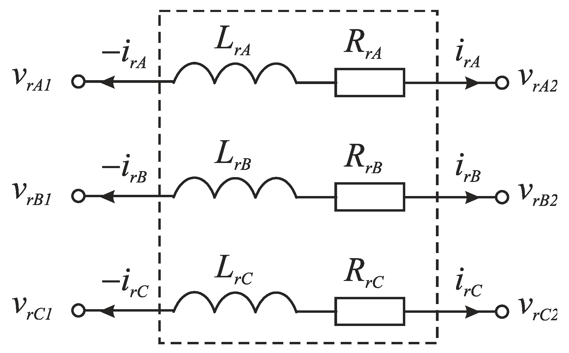
2.2. Mathematical Models of System’s Elements

To create a mathematical model of the power circuit of a thyristor voltage regulator (TVR), we make the following assumptions, which are characteristic of the well-known method of modeling power circuits of semiconductor converters as circuits with a constant structure and variable parameter. Each thyristor is represented by an electrical circuit of series-connected impedance and inductance. Their values for the switch-on state are taken so that the inheritance of the on-voltage on the circuit corresponds to the inheritance of the voltage on the switched-on thyristor, and the values for the switch-off state such that the current circuit can be neglected. The option of simultaneously opening two thyristors in phase is impossible. Thyristor switch-on occurs instantly when the thyristor opening condition, which is specified by a logical expression, is fulfilled. The thyristor switch-off is a step in which the current circuit changes its sign from positive (at the beginning of the step) to negative (at the end of the step), at the moment of the current circuit transition through 0. An increase in the equivalent resistance and inductance of the line at the moment when the line current is equal to 0 corresponds to the physical principles of thyristor operation and ensures the stability of the calculation. Note that the used method is distinguished by increased numerical stability, including parametric changes, which is substantiated, in particular, in [41,42]. Assuming a linear law of current change in step, this point in time can be calculated as

$$t\prime =t_0+\frac{i_0-i_1}{t_1-t_0}{i}_0$$

(7)

Taking into account these assumptions, the electrical circuit of the TRN as a six-terminal will follow the scheme shown in Figure 2.

After applying Equation (1) for the first-order AVIS method (m = 1) to the calculation scheme in Figure 2, we obtain the equation:

$$\begin{gathered} \frac{1}{\Delta t}\underset{t_0}{\overset{t_0+\Delta t}{\int }}{v}_{TVR1}^{}dt-\frac{1}{\Delta t}\underset{t_0}{\overset{t_0+\Delta t}{\int }}{v}_{TVR4}^{}dt-R_{T1}{i}_{T{1}_0}+\left(\frac{R_{T1}}{2}+\frac{L_{T1}}{\Delta t}\right)i_{T{1}_0}-\left(\frac{R_{T1}}{2}+\frac{L_{T1}}{\Delta t}\right)i_{T{1}_1}=0 \\ ,\frac{1}{\Delta t}\underset{t_0}{\overset{t_0+\Delta t}{\int }}{v}_{TVR4}^{}dt-\frac{1}{\Delta t}\underset{t_0}{\overset{t_0+\Delta t}{\int }}{v}_{TVR1}^{}dt-R_{T2}{i}_{T{2}_0}+\left(\frac{R_{T2}}{2}+\frac{L_{T2}}{\Delta t}\right)i_{T{2}_0}-\left(\frac{R_{T2}}{2}+\frac{L_{T2}}{\Delta t}\right)i_{T{2}_1}=0 \\ \frac{1}{\Delta t}\underset{t_0}{\overset{t_0+\Delta t}{\int }}{v}_{TVR2}^{}dt-\frac{1}{\Delta t}\underset{t_0}{\overset{t_0+\Delta t}{\int }}{v}_{TVR5}^{}dt-R_{T3}{i}_{T{3}_0}+\left(\frac{R_{T3}}{2}+\frac{L_{T3}}{\Delta t}\right)i_{T{3}_0}-\left(\frac{R_{T3}}{2}+\frac{L_{T3}}{\Delta t}\right)i_{T{3}_1}=0 \\ \frac{1}{\Delta t}\underset{t_0}{\overset{t_0+\Delta t}{\int }}{v}_{TVR5}^{}dt-\frac{1}{\Delta t}\underset{t_0}{\overset{t_0+\Delta t}{\int }}{v}_{TVR2}^{}dt-R_{T4}{i}_{T{4}_0}+\left(\frac{R_{T4}}{2}+\frac{L_{T4}}{\Delta t}\right)i_{T{4}_0}-\left(\frac{R_{T4}}{2}+\frac{L_{T4}}{\Delta t}\right)i_{T{4}_1}=0 \\ \frac{1}{\Delta t}\underset{t_0}{\overset{t_0+\Delta t}{\int }}{v}_{TVR3}^{}dt-\frac{1}{\Delta t}\underset{t_0}{\overset{t_0+\Delta t}{\int }}{v}_{TVR6}^{}dt-R_{T5}{i}_{T{5}_0}+\left(\frac{R_{T5}}{2}+\frac{L_{T5}}{\Delta t}\right)i_{T{5}_0}-\left(\frac{R_{T5}}{2}+\frac{L_{T5}}{\Delta t}\right)i_{T{5}_1}=0 \\ \frac{1}{\Delta t}\underset{t_0}{\overset{t_0+\Delta t}{\int }}{v}_{TVR6}^{}dt-\frac{1}{\Delta t}\underset{t_0}{\overset{t_0+\Delta t}{\int }}{v}_{TVR3}^{}dt-R_{T6}{i}_{T{6}_0}+\left(\frac{R_{T6}}{2}+\frac{L_{T6}}{\Delta t}\right)i_{T{6}_0}-\left(\frac{R_{T6}}{2}+\frac{L_{T6}}{\Delta t}\right)i_{T{6}_1}=0 \end{gathered}$$

(8)

where $v_{TVR1}^{}$—$v_{TVR6}^{}$—pole potentials; $i_{T1}^{}$—$i_{T6}^{}$—thyristor currents; $R_{T1}^{}$—$R_{T6}^{}$—resistances in circuit equivalent to thyristors; $L_{T1}^{}$—$L_{T6}^{}$—inductances of circuit equivalent to thyristors.

On the basis of Equation (8), write the external vector equation of TVR as multipole:

$${\overrightarrow{i}}_{TVR}+G_{TVR}\frac{1}{\Delta t}\underset{t_0}{\overset{t_0+\Delta t}{\int }}{\overrightarrow{v}}_{TVR}dt+{\overrightarrow{C}}_{TVR}=0$$

(9)

where ${\overrightarrow{i}}_{TVR}={\left(i_{TVR{1}_1},i_{TVR{2}_1},i_{TVR{3}_1},i_{TVR{4}_1},i_{TVR{5}_1},i_{TVR{6}_1}\right)}^T$—current vector of outer circuits on the end of integration step; moreover ${\overrightarrow{i}}_{TVR}={\left(i_{T{2}_1},i_{T{4}_1},i_{T{6}_1},i_{T{1}_1},i_{T{3}_1},i_{T{5}_1}\right)}^T$; ${\overrightarrow{v}}_{TVR}={\left(v_{TVR1},v_{TVR2},v_{TVR3},v_{TVR4},v_{TVR5},v_{TVR6}\right)}^T$—vector of pole potentials;

$$\begin{gathered} G_{TVR}=\left[\begin{array}{cccccc}{R}_{T2}^{*-1}& 0& 0& -R_{T2}^{*-1}& 0& 0\\ 0& R_{T4}^{*-1}& 0& 0& -R_{T4}^{*-1}& 0\\ 0& 0& R_{T6}^{*-1}& 0& 0& -R_{T6}^{*-1}\\ -R_{T1}^{*-1}& 0& 0& R_{T1}^{*-1}& 0& 0\\ 0& -R_{T3}^{*-1}& 0& 0& R_{T3}^{*-1}& 0\\ 0& 0& -R_{T5}^{*-1}& 0& 0& R_{T5}^{*-1}\end{array}\right], \\ {R}_{Ti}^{*}=\frac{R_{Ti}}{2}+\frac{L_{Ti}}{\Delta t},(i=1,2,3,4,5,6),{\overrightarrow{C}}_{TVR}=\left[\begin{array}{c}{R}_{T2}^{*-1}{R}_{T2}{i}_{T{2}_0}-i_{T{2}_0}\\ R_{T4}^{*-1}{R}_{T4}{i}_{T{4}_0}-i_{T{4}_0}\\ R_{T6}^{*-1}{R}_{T6}{i}_{T{6}_0}-i_{T{6}_0}\\ R_{T1}^{*-1}{R}_{T1}{i}_{T{1}_0}-i_{T{1}_0}\\ R_{T3}^{*-1}{R}_{T3}{i}_{T{3}_0}-i_{T{3}_0}\\ R_{T5}^{*-1}{R}_{T5}{i}_{T{5}_0}-i_{T{5}_0}\end{array}\right] \end{gathered}$$

(10)

Equation (9) is an algebraic equation that allows us to determine the currents of the thyristors at the end of the numerical integration step by the known pole potentials, power circuit parameters and initial conditions.

Note that the matrix of coefficients $G_{TVR}$ is determined by the parameters in the equivalent circuit to thyristors and must be calculated at each integration step. Similarly, the constant terms vector ${\overrightarrow{C}}_{TVR}$ must be calculated at each step. This vector is determined by the parameters in the circuit, which are equivalent to thyristors and the initial conditions.

The thyristor switch-on condition is a logical expression that becomes true when the thyristor voltage is positive, the thyristor is switch-off and there is permission to switch-on at the control angle (calculated from the moment when the thyristor voltage becomes positive).

According to the approach used, the calculation scheme of the three-phase choke is presented in six-terminal form (Figure 3).

Applying Equation (1) for the first-order AVIS method (m = 1) to the given calculation scheme, we will receive

$$\begin{gathered} \frac{1}{\Delta t}\underset{t_0}{\overset{t_0+\Delta t}{\int }}{v}_{rA1}^{}dt-\frac{1}{\Delta t}\underset{t_0}{\overset{t_0+\Delta t}{\int }}{v}_{rA2}^{}dt-R_{rA}{i}_{r{A}_0}+\left(\frac{R_{rA}}{2}+\frac{L_{rA}}{\Delta t}\right)i_{r{A}_0}-\left(\frac{R_{rA}}{2}+\frac{L_{rA}}{\Delta t}\right)i_{r{A}_1}=0, \\ \frac{1}{\Delta t}\underset{t_0}{\overset{t_0+\Delta t}{\int }}{v}_{rB1}^{}dt-\frac{1}{\Delta t}\underset{t_0}{\overset{t_0+\Delta t}{\int }}{v}_{rB2}^{}dt-R_{rB}{i}_{r{B}_0}+\left(\frac{R_{rB}}{2}+\frac{L_{rB}}{\Delta t}\right)i_{r{B}_0}-\left(\frac{R_{rB}}{2}+\frac{L_{rB}}{\Delta t}\right)i_{r{B}_1}=0, \\ \frac{1}{\Delta t}\underset{t_0}{\overset{t_0+\Delta t}{\int }}{v}_{rС1}^{}dt-\frac{1}{\Delta t}\underset{t_0}{\overset{t_0+\Delta t}{\int }}{v}_{rС2}^{}dt-R_{rС}{i}_{r{С}_0}+\left(\frac{R_{rС}}{2}+\frac{L_{rС}}{\Delta t}\right)i_{r{С}_0}-\left(\frac{R_{rС}}{2}+\frac{L_{rС}}{\Delta t}\right)i_{r{С}_1}=0, \end{gathered}$$

(11)

where $i_{rA1},i_{rB1},i_{rC1}$—choke phase currents at the end of the integration step; $i_{rA0},i_{rB0},i_{rC0}$—choke phase currents at the start of the integration step; $v_{rA1},v_{rB1},v_{rC1},v_{rA2},v_{rB2},v_{rC2}$—pole potentials; $R_{rA}$,$R_{rB}$,$R_{rС}$—active resistance in the choke phases; $L_{rA}$,$L_{rB}$,$L_{rС}$—the inductance of the choke.

Based on the system in Equation (11), we write the external vector equation for the choke as six-pole:

$${\overrightarrow{i}}_r+G_r\frac{1}{\Delta t}\underset{t_0}{\overset{t_0+\Delta t}{\int }}{\overrightarrow{v}}_{r}dt+{\overrightarrow{C}}_r=0,$$

(12)

where ${\overrightarrow{i}}_r={\left(-i_{rA1},-i_{rB1},-i_{rC1},i_{rA1},i_{rB1},i_{rC1}\right)}^T$—vector of currents in external circuits at the end of the integration step; ${\overrightarrow{v}}_r={\left(v_{rA1},v_{rB1},v_{rC1},v_{rA2},v_{rB2},v_{rC2}\right)}^T$—vector of potentials of the outer poles; G_r, C_r—the matrix of coefficients and the vector of free terms, respectively:

$$G_r=\left[\begin{array}{cccccc}R{*}_{rA}^{-1}& 0& 0& -R{*}_{rA}^{-1}& 0& 0\\ 0& R{*}_{rB}^{-1}& 0& 0& -R{*}_{rB}^{-1}& 0\\ 0& 0& R{*}_{rC}^{-1}& 0& 0& -R{*}_{rC}^{-1}\\ -R{*}_{rA}^{-1}& 0& 0& R{*}_{rA}^{-1}& 0& 0\\ 0& -R{*}_{rB}^{-1}& 0& 0& R{*}_{rB}^{-1}& 0\\ 0& 0& -R{*}_{rC}^{-1}& 0& 0& R{*}_{rC}^{-1}\end{array}\right],{\overrightarrow{C}}_r=\left[\begin{array}{c}{R}_{rA}^{*-1}{R}_{rA}{i}_{r{A}_0}-i_{r{A}_0}\\ R_{rB}^{*-1}{R}_{rB}{i}_{r{B}_0}-i_{r{B}_0}\\ R_{rC}^{*-1}{R}_{rC}{i}_{r{C}_0}-i_{r{C}_0}\\ -R_{rA}^{*-1}{R}_{rA}{i}_{r{A}_0}+i_{r{A}_0}\\ -R_{rB}^{*-1}{R}_{rB}{i}_{r{B}_0}+i_{r{B}_0}\\ -R_{rC}^{*-1}{R}_{rC}{i}_{r{C}_0}+i_{r{C}_0}\end{array}\right];$$

$R{*}_{rA}=\frac{R_{rA}}{2}+\frac{L_{rA}}{\Delta t}$,$R{*}_{rB}=\frac{R_{rB}}{2}+\frac{L_{rB}}{\Delta t}$, $R{*}_{rC}=\frac{R_{rC}}{2}+\frac{L_{rC}}{\Delta t}$ step resistances.

From Equation (12), according to the known pole potentials, choke parameters and initial conditions, we determine the choke currents at the end of the numerical integration step.

Next, consider the mathematical model of a short network with furnace space (arc). In [17], using the 1st order AVIS method, the following algebraic equation was obtained to determine the current in circuit with an electric arc:

$$i_1=i_0+{\left(\frac{R+R_{d0}}{2}+\frac{L}{\Delta t}\right)}^{-1}\left(U-R{i}_0-u_{arc0}\right),$$

(13)

where i₀, i₁—the value of the circuit current at the beginning and end of the numerical integration step; R_d0—dynamic resistance of the arc; R—resistance of circuit; L—circuit inductance; $U=\frac{1}{\Delta t}\underset{t_0}{\overset{t_0+\Delta t}{\int }}udt$—the average value of the applied voltage at the integration step, u_arc0—the value of the arc voltage at the beginning of the integration step. We calculate the instantaneous values of the arc voltage at each integration step according to the formula

$$u_{arc1}=u_{arc0}+R_d\Delta i,$$

(14)

where $\Delta i=i_1-i_0$—arc current increase in step.

The dynamic resistance of the arc is calculated at each step of numerical integration by the volt-ampere characteristics in the arc [17]. To calculate the dynamic resistance of the arc depending on the magnitude of the arc current I_arc and its length l_arc, in [17], the authors proposed the use of the following approximations used in this model:

$$\mathrm{if}{I}_{arc}\cdot \frac{d{I}_{arc}}{dt}>0\mathrm{then}$$

$$R_d\left(I_{arc}, l_{arc}\right)=\frac{0.4337}{\sqrt{\sigma \left( l_{arc}\right)}}\cdot a_{11}\left( l_{arc}\right)\cdot \left(1-{\left(\frac{I_{arc}}{\sigma \left( l_{arc}\right)\cdot a_{21}\left( l_{arc}\right)}\right)}^2\right)exp\left(-a_{31}\left( l_{arc}\right)\cdot {\left(\frac{I_{arc}}{\sigma \left( l_{arc}\right)}\right)}^{2\cdot a_{41}\left( l_{arc}\right)}\right),$$

(15)

$$\mathrm{if}{I}_{arc}\cdot \frac{d{I}_{arc}}{dt}<0\mathrm{then}{R}_d\left(I_{arc},l_{arc}\right)=a_0\left( l_{arc}\right)\cdot \left(1-\left(th{\left(\frac{I_{arc}}{\sigma \left( l_{arc}\right)\cdot 0.5}\right)}^2\right)\right),$$

(16)

where $a_{11}\left( l_{arc}\right)=0.9658\cdot l_{arc}-0.1282$;

$$\begin{array}{l}{a}_{21}\left( l_{arc}\right)=2.0477\cdot {10}^{-5}\cdot l_{arc}{}^3-0.0005\cdot l_{arc}{}^2+0.0019\cdot l_{arc}+0.3992;\\ a_{31}\left( l_{arc}\right)=-0.0026\cdot l_{arc}{}^3+0.0939\cdot l_{arc}{}^2-0.3429\cdot l_{arc}+14.0293;\\ a_{41}\left( l_{arc}\right)=2;\\ \sigma \left( l_{arc}\right)=\left(0.0093\cdot l_{arc}{}^2-0.4513\cdot l_{arc}+9.2986\right)\cdot 10000;\\ a_0\left( l_{arc}\right)=\left(0.0004\cdot l_{arc}{}^4-0.0124\cdot l_{arc}{}^3+0.1468\cdot l_{arc}{}^2+0.0081\cdot l_{arc}+0.1418\right)/1000.\end{array}$$

According to the approach used, a short network with furnace space (arc) is represented as six-pole (Figure 4) and is described by an external vector equation of the form (17), obtained on the basis of Equation (1).

$${\overrightarrow{i}}_{SL}+G_{SL}\frac{1}{\Delta t}\underset{t_0}{\overset{t_0+\Delta t}{\int }}{\overrightarrow{v}}_{SL}dt+{\overrightarrow{C}}_{SL}=0,$$

(17)

where ${\overrightarrow{i}}_{SL}={\left(i_{SLA1},i_{SLB1},i_{SLC1},i_{SLA2},i_{SLB2},i_{SLC2}\right)}^T$—current vector of outer circuits; $\frac{1}{\Delta t}\underset{t_0}{\overset{t_0+\Delta t}{\int }}{\overrightarrow{v}}_{SL}dt$—averages of the values for the potentials of the poles at the numerical integration step; ${\overrightarrow{v}}_{SL}=\left(\begin{array}{c}{\overrightarrow{v}}_{SL1}\\ {\overrightarrow{v}}_{SL2}\end{array}\right)$, ${\overrightarrow{v}}_{SL1}={\left(v_{SLA1},v_{SLB1},v_{SLC1}\right)}^T$, ${\overrightarrow{v}}_{SL2}={\left(v_{SLA2},v_{SLB2},v_{SLC2}\right)}^T$- pole potential vectors and coefficient matrices:

$$G_{SL}=\left[\begin{array}{cccccc}R{*}_{SLA}^{-1}& 0& 0& -R{*}_{LA}^{-1}& 0& 0\\ 0& R{*}_{LB}^{-1}& 0& 0& -R{*}_{LB}^{-1}& 0\\ 0& 0& R{*}_{LC}^{-1}& 0& 0& -R{*}_{LC}^{-1}\\ -R{*}_{LA}^{-1}& 0& 0& R{*}_{LA}^{-1}& 0& 0\\ 0& -R{*}_{LB}^{-1}& 0& 0& R{*}_{LB}^{-1}& 0\\ 0& 0& -R{*}_{LC}^{-1}& 0& 0& R{*}_{LC}^{-1}\end{array}\right],$$

$${\overrightarrow{C}}_{SL}=\left[\begin{array}{c}-R{*}_{SLA}^{-1}\left(R_{SLA}{i}_{SLA0}+u_{arcA0}\right)+i_{SLA0}\\ -R{*}_{SLB}^{-1}\left(R_{SLB}{i}_{SLB0}+u_{arcB0}\right)+i_{SLB0}\\ -R{*}_{SLC}^{-1}\left(R_{SLC}{i}_{SLC0}+u_{arcC0}\right)+i_{SLC0}\\ R{*}_{SLA}^{-1}\left(R_{SLA}{i}_{SLA0}-u_{arcA0}\right)-i_{SLA0}\\ R{*}_{SLB}^{-1}\left(R_{SLB}{i}_{SLB0}-u_{arcB0}\right)-i_{SLB0}\\ R{*}_{SLC}^{-1}\left(R_{SLC}{i}_{SLC0}-u_{arcC0}\right)-i_{SLC0}\end{array}\right],$$

$R{*}_{SLA}=\frac{R_{SLA}+R_{dA0}}{2}+\frac{L_{SLA}}{\Delta t}$; $R{*}_{SLB}=\frac{R_{SLB}+R_{dB0}}{2}+\frac{L_{SLB}}{\Delta t}$, $R{*}_{SLC}=\frac{R_{SLC}+R_{dC0}}{2}+\frac{L_{SLC}}{\Delta t}$ —step resistance of phases, $i_{SLA}=-i_{SLA1}=i_{SLA2}$, $i_{SLB}=-i_{SLB1}=i_{SLB2}$, $i_{SLC}=-i_{SLC1}=i_{SLC2}$—phase currents (arc currents).

Equation (17) is used to determine the phase currents in a short network with furnace space (arc currents) according to the dynamic arc resistances, which are determined from approximation Equations (12) and (13), determined with (11) values of arc voltages and power circuit parameters and initial conditions. Mathematical models of a three-phase power supply network and a three-phase transformer are described in [17].

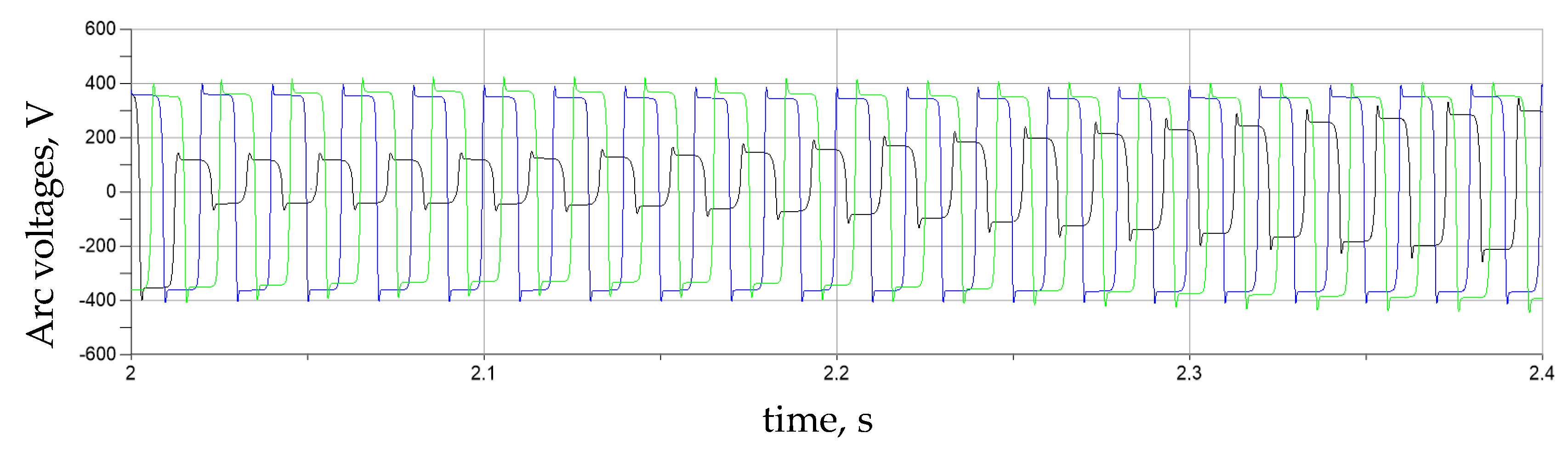
2.3. The Model Verification

To verify the adequacy of the developed model, calculations for the steady-state symmetric modes and the perturbation mode of the arc length in one phase, during which there was a sharp decrease in the arc length in phase A (from 16 mm to 4 mm), were performed.

The simulation results were compared with the results of analytical calculations and experimental studies presented in [31]. The results of the calculation for asymmetric perturbation of the arc length mode are shown in Figure 5 and Figure 6. As a result, there was a sharp decrease in arc voltage in phase A (Figure 5) and an increase in current in phase A that affected the value of currents in other phases, where the perturbation in the lengths of the arcs was absent (Figure 6).

Table 1. Comparison of the calculation results of arc currents with the results of the experiment: I_A, I_B, I_C—arc current effective values, I_A0, I_B0, I_C0—constant components of arc currents.

Operation Mode	Phase A				Phase B				Phase C
	IA, kA		IA0, kA		IB, kA		IB0, kA		IC, kA		IC0, kA
	Mod	Exp	Mod	Exp	Mod	Exp	Mod	Exp	Mod	Exp	Mod	Exp
Switched 3 arcs (symmentrical mode)	62.7	64.5	-	-	62.8	65.0	-	-	63.5	66.0	-	-
Onephase short circuit on phase A	80.0	81.0	−3.8	−3.2	59.2	60.0	1.7	1.5	70.0	76.0	1.4	1.65

compares the calculated values of arc currents in the symmetric mode and in the short-circuit mode in phase A and the experimental results published in [31]. Comparing the results suggests adequacy in terms of the calculation.

Note that in [17], a mathematical model for the ASF power supply system without an adjustable reactor was described. The adequacy of such a system was confirmed in [17] by way of comparison with experimental data. In the presented study, this model is supplemented with an adjustable reactor (MTVR), so we will focus on the validation of the model in the part of the power system with an adjustable reactor. Such validation was carried out by comparing it with the data for analytical calculations.

In [31], an analytical equation for choke MTVR current was obtained

$$i_2=e^{-\frac{R_r}{X_r}\omega t}\left(I_m\mathit{sin}\left(\alpha \right)-\frac{E_T}{R_r}\right)+\frac{E_T}{R_r},$$

where R_r, X_r—active and reactive choke resistance, I_m—choke current amplitude, E_T—switch-on thyristor voltage, α—thyristor opening angle.

On the basis of an analytical description in [31], time diagrams for the choke current for different values of γ = R_r/X_r, as well as the mains current, are drawn (Figure 7). In this case, the assumption of a trapezoidal form for the choke current is accepted. In Figure 8, for comparison, the same values are obtained by computer simulation using the developed model. As can be seen, the shape of the choke current and the shape of the mains current according to the results of computer simulation correspond to known analytical dependences. This confirms the adequacy of the developed model for the power circuit with MTVR.

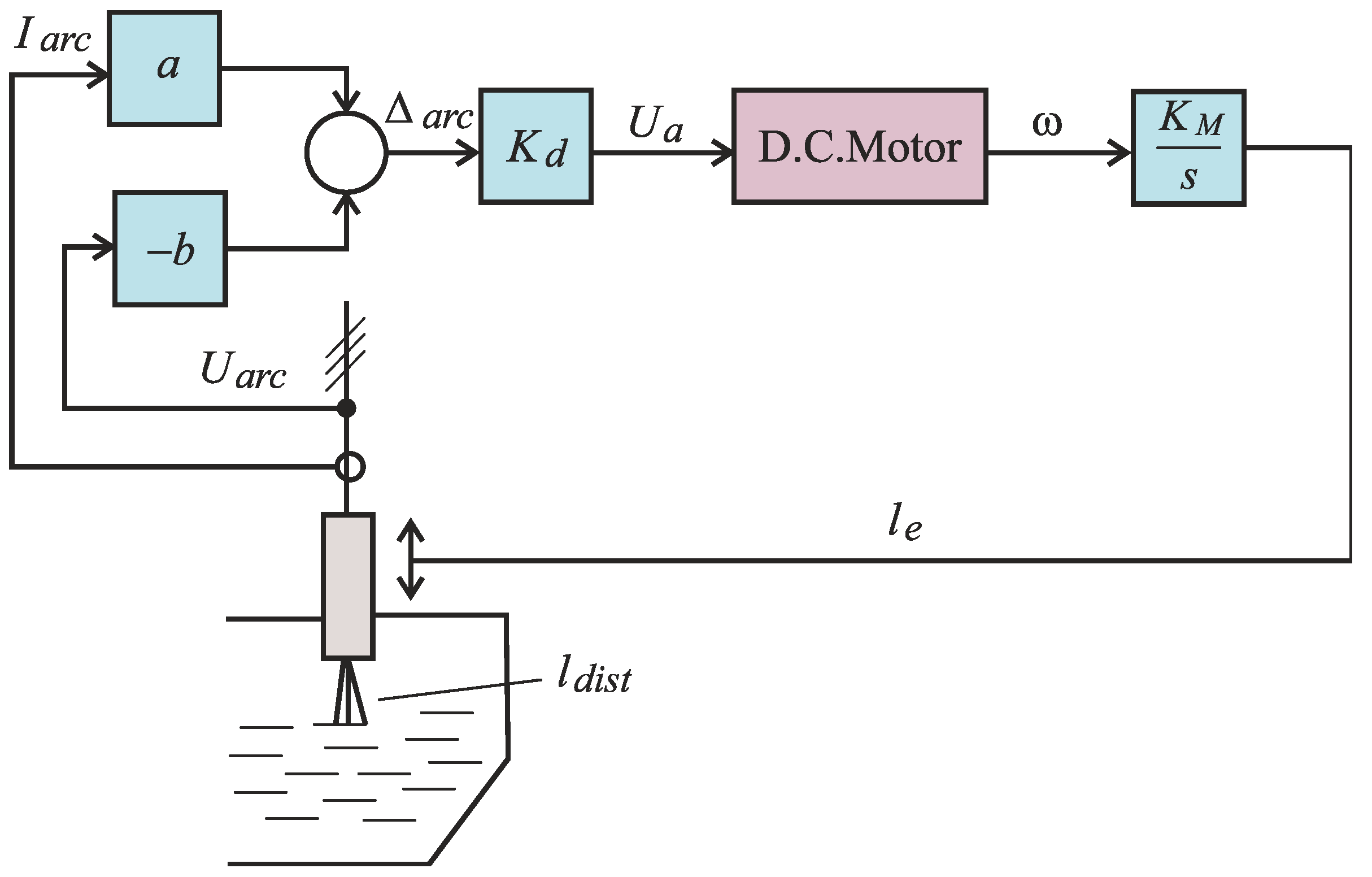
3. The Electrode Movement System

A functional diagram of the electrode movement system is shown in Figure 9.

The movement of the electrodes is carried out by a DC electric drive. In conducting research, we used the impedance control principle, according to which the control signal in the electric drive is boosted based on the current values. I_arc and arc voltage U_arc are calculated by the equations

$${\Delta }_{arc}=a{I}_{arc}-b{U}_{arc}\mathrm{and}\mathrm{if}{\Delta }_{arc}=0\mathrm{then}\frac{U_{arc}}{I_{arc}}=\frac{a}{b}.$$

(18)

This control law provides optimal power control with a certain adjustment in the coefficients a and b. Given that at the extreme point

$$\frac{d{P}_{arc}}{d{I}_{arc}}=U_{arc}+I_{arc}\frac{d{U}_{arc}}{d{I}_{arc}}=0\mathrm{and}\mathrm{then}\frac{U_{arc}}{I_{arc}}=-\frac{d{U}_{arc}}{d{I}_{arc}}$$

(19)

According to [44], the electrical circuit of the ASF in a single-phase substitution circuit consists of three elements: the arc gap in the form of variable active arc resistance R_arc and reduced to the secondary winding of the transformer total active R_∑ and reactive resistance X_∑, which take into account the resistances of the furnace transformer with the reactor, short network with electrode and melt. Then:

$$U_{arc}=\sqrt{U_{2phase}^2-I_{arc}^2\cdot X_{\Xi }^2}-I_{arc}\cdot R_{\Xi }$$

(20)

and, respectively:

$$\frac{\partial U_{arc}}{\partial I_{arc}}=\frac{-I_{arc}\cdot X_{\Xi }^2}{\sqrt{U_{2phase}^2-I_{arc}^2\cdot X_{\Xi }^2}}-R_{\Xi }=\frac{-X_{\Xi }^2}{R_{arc}+R_{\Xi }}-R_{\Xi }.$$

(21)

Then, substituting (21) into (19), we obtain

$$\frac{U_{arc}}{I_{arc}}=\frac{X_{\Xi }^2}{R_{arc}+R_{\Xi }}+R_{\Xi }=\frac{X_{\Xi }^2+R_{\Xi }\cdot \left(R_{arc}+R_{\Xi }\right)}{R_{arc}+R_{\Xi }}.$$

(22)

On the other hand, as shown in [22], the power extremum $\frac{d{P}_{arc}}{d{R}_{arc}}=0$ when $R_{arc}=\sqrt{R_{\Xi }^2+X_{\Xi }^2}$ and after i пicля substitutions in Equation (22), we obtain:

$$\frac{U_{arc}}{I_{arc}}=\frac{X_{\Xi }^2+R_{\Xi }\cdot \left(\sqrt{R_{\Xi }^2+X_{\Xi }^2}+R_{\Xi }\right)}{\sqrt{R_{\Xi }^2+X_{\Xi }^2}+R_{\Xi }}.$$

(23)

Taking into account (18), the coefficients of the regulator, which theoretically provide extreme control, can be determined on the basis of (23) as

$$a=\gamma \cdot \left(X_{\Xi }^2+R_{\Xi }\cdot \left(\sqrt{R_{\Xi }^2+X_{\Xi }^2}+R_{\Xi }\right)\right)$$

$$b=\gamma \cdot \left(\sqrt{R_{\Xi }^2+X_{\Xi }^2}+R_{\Xi }\right)$$

where γ—scaling factor.

As shown in [45], the inductive resistance varies $X_{\Xi }$ depending on the stage of melting, which requires a corresponding change in the coefficients. The change in inductive resistance $X_{\Xi }$ is proposed to take into account the following equation

$$X_{\Xi }=X_{sh}\cdot {\left(\frac{I_{arc}}{I_{sh}}\right)}^{-k}$$

where $I_{sh}$, $X_{sh}$—current and inductive resistance in short-circuit mode; k—factor that depends on the melting stage, in particular, at the beginning of the melt $k=0.5÷0.6$, in the case of burning the arc on the lake of molten metal at the stage of penetration of wells $k=0.25÷0.3$ and when burning the arc on the molten metal $k=0$.

A mathematical model for the electrode movement system created using the 1st-order AVIS method is described in [17].

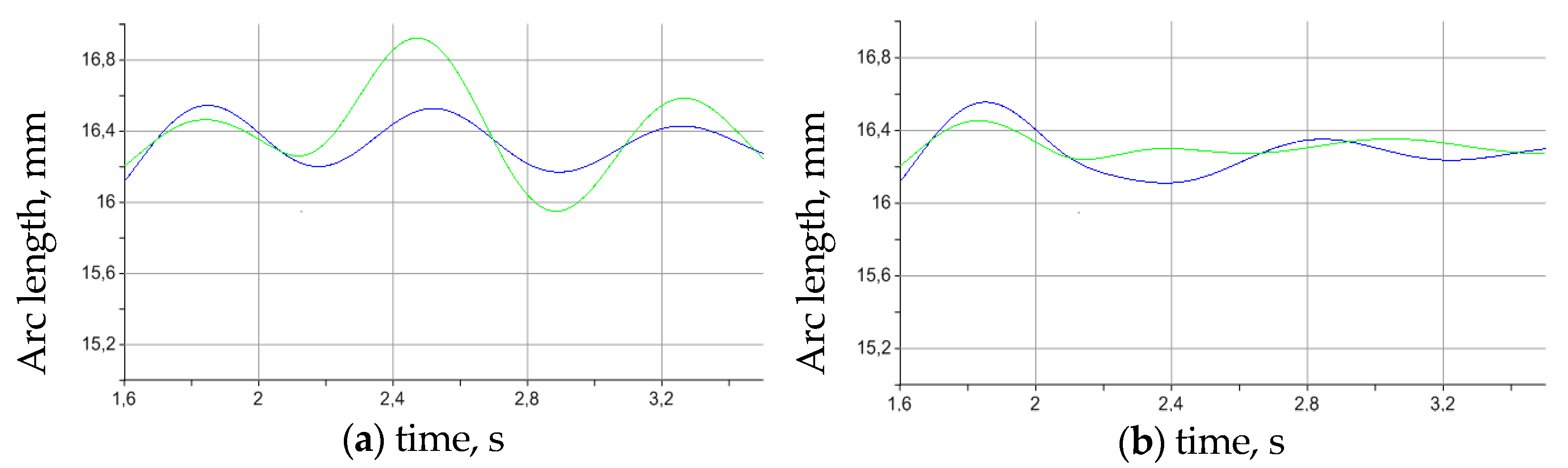
4. Researches Results of Regulation Modes of MTVR

The objectives of the research were: analysis of asymmetric perturbations in the furnace space, establishment of reactor control laws in the high-speed arc control circuit, analysis of the interaction of the high-speed arc control circuit and the electrode movement control circuit, analysis of the controlled reactor impact on the network.

As a result of the perturbation, there is a mismatch signal in the control system of the electrodes (see Equation (18)), resulting in a control signal to move the electrodes, which provides recovery of arc length and operating point of arc combustion (arc impedance). Note that changing the magnitude of arc currents in phases where there are no perturbations causes a mismatch signal in the control system of the electrodes of these phases, which causes incorrect electrode movements and changes in arc length in these phases. Stabilizing the length of the arcs is an important task in the automatic control system.

The thyristor-controlled choke is able to regulate the supply current with high speed and, hence, the arc current. One way to control the choke is to control the current, the task of which is to stabilize the arc currents. In this case, the control signal by thyristors is formed by the PI controller as a function of the deviation in the current value from the setpoint.

Below are given the results of studies on the perturbation mode of the arc length in one phase, during which there was a sharp decrease in the arc length in phase A. Oscillograms of instantaneous values for arc currents with MTVR regulation as a function of current, in which the alignment of arc currents is noticeable, especially at the beginning of perturbation, are shown in Figure 10.

The thyristor-controlled choke effectively stabilizes the current value of arc currents (Figure 11). As a result, arc lengths are stabilized in phases where perturbation is absent (Figure 12 and Figure 13). The fact of stabilization in the arc length is especially noticeable for phases where currents increase (phases A and C). Slightly smaller (but also noticeable) is the effect for phase B, where the current changes less. At the same time, current stabilization reduces the control action of the electrode movement system, because when the current decreases under the action of a controlled choke, the mismatch signal decreases Δ_arc (18). This slows down (almost twice) the recovery of the arc length in the phase where the perturbation exists, although it reduces the fluctuations in the transient mode (Figure 11a). Slowing down the control circuit of the electrode movement under the influence of the high-speed current control circuit is a disadvantage of this method for choke control.

To ensure maximum power in the arc, it is necessary to stabilize the specified ratio between voltage and arc current (arc impedance), determined from (18). With this in mind, combined choke control is proposed. In this control, in the area of significant discrepancies Δ_arc (at the beginning of the perturbation, with a significant change in the power of the arc), control of the inductor is carried out as a function of mismatch, and in the area of small deviations—as a function of current. In Figure 14 are shown the change in the Δ_arc mismatch when using choke current control and combined control.

Table 2. The standard deviation for the Δ_arc mismatch when using different throttle control methods.

Control Methode	Standard Deviation Δarc = aIarc − bUarc from 0
Whithout MTVR	4.64
Control by arc currents	3.7
Combine control of MTVR	3.1

provides the standard deviation for the Δ_arc mismatch when using different choke control methods. The results show that from the point of view of minimizing the standard deviation Δarc, the combined law of choke control provides better results in comparison with the classical control of arc currents, although the current asymmetry is greater.

Another research task was to analyze the influence of the thyristor regulator in the high-speed control circuit on the power supply network. Harmonic analysis of mains currents was performed using functions Matlab fft, thd. In Figure 15a, the harmonic spectrum of the mains current in the absence of thyristor-controlled choke for steady-state symmetrical mode is described. In this case, the distortions are insignificant and are due only to the nonlinear nature of the load (arc), as the coefficient of harmonic distortion is equal to THD = 0.2%.

In Figure 15b, the harmonic current spectrum phase A with thyristor-controlled choke, in the case of the combined principle of choke control at the beginning of the perturbation, when there is a maximum control action, is shown. In this case, the control angle of the thyristors is set to the maximum (in this case 100°) and there is a complete introduction of the choke in phase A (thyristors in phase A is switched off). In this mode, the current distortion is slightly increased (THDA = 0.7%). The coefficients of harmonic distortion of the currents in phases B and C are, respectively, THDB = 0.66%, THDC = 0.8%.

Figure 16 shows the harmonic spectrum of mains currents (phase A, B, C) with current regulation of the choke at the beginning of the perturbation, when the maximum control action takes place. As can be seen from the presented results, the distortion in mains currents, in this case, depends on the switched angle of the thyristors, which is different for different phases. Increasing this angle causes an increase in the coefficient of harmonic distortion. At small switched angles of thyristors in phase C (choke is almost shunted), current distortions are insignificant.

The average value of the harmonic distortion coefficient for the currents in the network phases over the entire control interval for different ways of controlling the choke are given in

Table 3. The average value of the harmonic distortion coefficient of the currents of the network phases throughout the studied control interval for different methods of choke control.

Control Method of MTVR	THD, %
	Phase A	Phase B	Phase C
Current control	0.19	0.198	0.2
Combine control	0.41	0.13	0.31
Without MTVR	0.088	0.07	0.07

. As can be seen from the results, the thyristor-controlled choke introduces some distortions in mains currents, which are greater in the case of using a combined method of choke control. This is due to the greater control effect on the thyristor regulator at the beginning of the perturbation during impedance control.

5. Conclusions

Created using the AVIS method, the mathematical model for the thyristor-controlled choke power supply system considers the power circuit as a circuit with constant structure and variable parameters and allows one to analyze electromagnetic processes in the chipboard power supply system, taking into account the interactions of electromechanical electrode movement power supply, as well as to analyze the impact of the controlled choke on the power supply network, which is manifested in the distortion in mains currents. The adequacy of the developed model is confirmed by comparison with analytical calculations and experimental data. The model has a high speed of calculation and can be used for synthesize control laws.

A high-speed current control circuit with thyristor-controlled choke allows you to adjust the supply currents in the chipboard, stabilizing them in the event of perturbations in the arc length and introducing relatively small harmonic distortion.

As the research results show, the use of the known principle of choke control in high-speed current control circuits with arc current stabilization affects the operation of the electrode movement system, slowing down its action. This has a negative effect on stabilization in the lengths of arcs during disturbances.

To ensure the maximum power of arcs is necessary, arc impedance stabilization, a comparative analysis on the reactor control methods showed that from the point of view of arc impedance stabilization, the best result is provided by the proposed combined method of choke control, when in case of significant perturbations of the arc length, the control is carried out by impedance, and in the zone of small deviations—in current function.

The interaction between the high-speed current control circuit and the electromechanical electrode movement system requires further research to synthesize their control laws to improve the quality of control.

References

1. Kim, J.; Sovacool, B.K.; Bazilian, M.; Griffiths, S.; Lee, J.; Yang, M.; Lee, J. Decarbonizing the iron and steel industry: A systematic review of sociotechnical systems, technological innovations, and policy options. Energy Res. Soc. Sci. 2022, 89, 102565. [Google Scholar] [CrossRef]
2. Ren, M.; Lu, P.; Liu, X.; Hossain, M.S.; Fang, Y.; Hanaoka, T.; O’Gallachoir, B.; Glynn, J.; Dai, H. Decarbonizing China’s iron and steel industry from the supply and demand sides for carbon neutrality. Appl. Energy 2021, 298, 117209. [Google Scholar] [CrossRef]
3. Lee, B.; Sohn, I. Review of Innovative Energy Savings Technology for the Electric Arc Furnace. JOM 2014, 66, 1581–1594. [Google Scholar] [CrossRef]
4. Köhle, S.; Madill, J.; Lichterbeck, R. Optimisation of High Voltage AC Electric Arc Furnace Control: Final Report; Directorate-General for Research and Innovation; Publications Office, European Commission: Brussels, Belgium, 2002. [Google Scholar]
5. Panoiu, M.; Panoiu, C.; Deaconu, S. Study about the possibility of electrodes motion control in the EAF based on adaptive impedance control. In Proceedings of the 13th International Power Electronics and Motion Control Conference, Poznan, Poland, 1–3 September 2008; pp. 1409–1415. [Google Scholar]
6. Lozynskyi, O.; Paranchuk, Y.; Moroz, V.; Stakhiv, P. Computer Model of the Electromechanical System of Moving Electrodes of an Arc Furnace with a Combined Control Law. In Proceedings of the 2019 IEEE 20th International Conference on Computational Problems of Electrical Engineering (CPEE), Lviv-Slavske, Ukraine, 15–18 September 2019; pp. 1–5. [Google Scholar]
7. Ghiormez, L.; Prostean, O. Electric arc current control for an electric arc furnace based on fuzzy logic. In Proceedings of the IEEE 10th Jubilee International Symposium on Applied Computational Intelligence and Informatics, Timisoara, Romania, 21–23 May 2015; pp. 359–364. [Google Scholar]
8. Parsapoor, A.; Ataei, M.; Kiyoumarsi, A. Adaptive control of the electric arc furnace electrodes using Lyapunov design. In Proceedings of the International Conference on Control, Automation and Systems, Seoul, Korea, 17–20 October 2007; pp. 1617–1622. [Google Scholar]
9. Lozynskyi, A.O.; Paranchuk, J.S.; Demkiv, L.I. Investigation of the electrodes movement system of arc furnace fuzzy controller. Tech. Electrodyn. 2014, 2, 73–77. [Google Scholar]
10. Paranchuk, Y.; Shabatura, Y.; Kuznyetsov, O. The Electrodes Positioning Control System for the Electric Arc Furnace Basing on Fuzzy Logic. In Proceedings of the IEEE International Conference on Modern Electrical and Energy Systems (MEES), Kremenchuk, Ukraine, 21–24 September 2021; pp. 1–5. [Google Scholar]
11. Taslimian, M.; Shabaninia, F.; Vaziri, M.; Vadhva, S. Fuzzy type-2 electrode position controls for an Electric Arc Furnace. In Proceedings of the IEEE 13th International Conference on Information Reuse & Integration (IRI), Las Vegas, NV, USA, 8–10 August 2012; pp. 498–501. [Google Scholar]
12. Hong, Z.; Sheng, Y.; Kasuga, J.; Li, M.; Zhao, L. Development of AC Electric Arc-Furnace Control System Based on Fuzzy Neural Network. In Proceedings of the International Conference on Mechatronics and Automation, Luoyang, China, 25–28 June 2006; pp. 2459–2464. [Google Scholar]
13. Moghadasian, M.; Alenasser, E. Modelling and Artificial Intelligence-Based Control of Electrode System for an Electric Arc Furnace. Electromagn. Anal. Appl. 2011, 3, 47–55. [Google Scholar] [CrossRef] [Green Version]
14. Lozynskyy, O.; Lozynskyi, A.; Paranchuk, Y.; Biletskyi, Y. Optimal control of the electrical mode of an arc furnace on the basis of the three-dimensional vector of phase currents. Math. Modeling Comput. 2019, 6, 69–76. [Google Scholar] [CrossRef]
15. Logar, V.; Dovžan, D.; Škrjanc, I. Mathematical Modeling and Experimental Validation of an Electric Arc Furnace. ISIJ Int. 2011, 51, 382–391. [Google Scholar] [CrossRef] [Green Version]
16. Hocine, L.; Yacine, D.; Kamel, B.; Samira, K.M. Improvement of electrical arc furnace operation with an appropriate model. Energy 2009, 34, 1207–1214. [Google Scholar] [CrossRef]
17. Lozynskyy, A.; Kozyra, J.; Łukasik, Z.; Kuśmińska-Fijałkowska, A.; Kutsyk, A.; Paranchuk, Y.; Kasha, L. A Mathematical Model of Electrical Arc Furnaces for Analysis of Electrical Mode Parameters and Synthesis of Controlling Influences. Energies 2022, 15, 1623. [Google Scholar] [CrossRef]
18. Gerling, R.; Louis, T.; Schmeiduch, G.; Sesselmann, R.; Sieber, A. Optimizing the melting process at AC-EAF with neural networks. Metall 1999, 53, 410–418. [Google Scholar]
19. Wieczorek, T.; Mązka, K. Modeling of the AC-EAF process using computational intelligence methods. Electrotech. Rev. 2008, 11, 184–188. [Google Scholar]
20. Garcia-Segura, R.; Vázquez Castillo, J.; Martell-Chavez, F.; Longoria-Gandara, O.; Ortegón Aguilar, J. Electric Arc Furnace Modeling with Artificial Neural Networks and Arc Length with Variable Voltage Gradient. Energies 2017, 10, 1424. [Google Scholar] [CrossRef]
21. Zheng, W.; Xianmin, M. Model Predictive Control Based on Improved DBD Algorithm and Application of Electrode Control in EAF. In Proceedings of the Second International Conference on Intelligent Computation Technology and Automation, Changsha, China, 10–11 October 2009; pp. 806–809. [Google Scholar]
22. Martell-Chávez, F.; Ramírez-Argáez, M.; Llamas-Terres, A.; Micheloud-Vernackt, O. Theoretical Estimation of Peak Arc Power to Increase Energy Efficiency in Electric Arc Furnaces. ISIJ Int. 2013, 53, 743–750. [Google Scholar] [CrossRef] [Green Version]
23. Łukasik, Z.; Olczykowski, Z. Estimating the Impact of Arc Furnaces on the Quality of Power in Supply Systems. Energies 2020, 13, 1462. [Google Scholar] [CrossRef] [Green Version]
24. Olczykowski, Z. Electric Arc Furnaces as a Cause of Current and Voltage Asymmetry. Energies 2021, 14, 5058. [Google Scholar] [CrossRef]
25. Olczykowski, Z. Arc Voltage Distortion as a Source of Higher Harmonics Generated by Electric Arc Furnaces. Energies 2022, 15, 3628. [Google Scholar] [CrossRef]
26. Pires, I.A.; Cardoso, M.M.G.; Cardoso Filho, B.J. An Active Series Reactor for an Electric Arc Furnace: A Flexible Alternative for Power-Flow Control. IEEE Ind. Appl. Mag. 2016, 22, 53–62. [Google Scholar] [CrossRef]
27. Pires, I.A.; Machado, A.; Murta, M.; Cardoso Filho, B.d.J. Experimental results of a Thyristor Switched Series Reactor for Electric Arc Furnaces. In Proceedings of the IEEE Industry Applications Society Annual Meeting, Portland, OR, USA, 2–6 October 2016; pp. 1–5. [Google Scholar]
28. Cardoso, M.M.G.; Cardoso Filho, B.J. Thyristor Switched Series Reactor for Electric Arc Furnaces. In Proceedings of the Conference Record of the 2006 IEEE Industry Applications Conference Forty-First IAS Annual Meeting, Tampa, FL, USA, 8–12 October 2006; pp. 124–130. [Google Scholar]
29. Samet, H.; Ghanbari, T.; Ghaisari, J. Maximum Performance of Electric Arc Furnace by Optimal Setting of the Series Reactor and Transformer Taps Using a Nonlinear Model. IEEE Trans. Power Deliv. 2015, 30, 764–772. [Google Scholar] [CrossRef]
30. Lozinskii, O.Y.; Paranchuk, Y.S. System for the optimum control of the electrical conditions of an arc furnace powered through a controlled reactor. Russ. Metall. 2007, 2007, 737–743. [Google Scholar] [CrossRef]
31. Kostyniuk, L.D.; Lozynskyy, A.O.; Lozynskyy, O.Y.; Malyar, A.V.; Marushchak, Y.U.; Paranchuk, Y.S. Situational Control in Arc Steel-Melting Furnaces, Lviv; Lviv Polytechnic Publishing House: Lviv, Ukraine, 2004; p. 382. (In Ukrainian) [Google Scholar]
32. Sjarov, M.; Lechler, T.; Fuchs, J.; Brossog, M.; Selmaier, A.; Faltus, F.; Donhauser, T.; Franke, J. The Digital Twin Concept in Industry—A Review and Systematization. In Proceedings of the 25th IEEE International Conference on Emerging Technologies and Factory Automation (ETFA), Vienna, Austria, 8–11 September 2020; pp. 1789–1796. [Google Scholar]
33. Classens, K.; Heemels, W.P.M.H.M.; Oomen, T. Digital Twins in Mechatronics: From Model-based Control to Predictive Maintenance. In Proceedings of the IEEE 1st International Conference on Digital Twins and Parallel Intelligence (DTPI), Beijing, China, 15 July–15 August 2021; pp. 336–339. [Google Scholar]
34. Brosinsky, C.; Westermann, D.; Krebs, R. Recent and prospective developments in power system control centers: Adapting the digital twin technology for application in power system control centers. In Proceedings of the IEEE International Energy Conference (ENERGYCON), Limassol, Cyprus, 3–7 June 2018; pp. 1–6. [Google Scholar]
35. Morello, S.; Gnesda, J.; Dionise, T.J. Arc Furnace Performance Validation: Using Modeling, Monitoring, and Statistical Analysis. IEEE Ind. Appl. Mag. 2019, 25, 95–103. [Google Scholar] [CrossRef]
36. Kłosowski, Z.; Cieślik, S. The Use of a Real-Time Simulator for Analysis of Power Grid Operation States with a Wind Turbine. Energies 2021, 14, 2327. [Google Scholar] [CrossRef]
37. Kutsyk, A.; Semeniuk, M.; Korkosz, M.; Podskarbi, G. Diagnosis of the Static Excitation Systems of Synchronous Generators with the Use of Hardware-In-the-Loop Technologies. Energies 2021, 14, 6937. [Google Scholar] [CrossRef]
38. Kutsyk, A.; Lozynskyy, A.; Vantsevitch, V.; Plakhtyna, O.; Demkiv, L. A Real-Time Model of Locomotion Module DTC Drive for Hardware-In-The-Loop Implementation. Przegląd Elektrotechniczny 2021, 97, 60–65. [Google Scholar] [CrossRef]
39. Kavousi-Fard, A.; Khosravi, A.; Nahavandi, S. Reactive Power Compensation in Electric Arc Furnaces Using Prediction Intervals. IEEE Trans. Ind. Electron. 2017, 64, 5295–5304. [Google Scholar] [CrossRef]
40. Plakhtyna, O.; Kutsyk, A.; Semeniuk, M.; Kuznyetsov, O. Object-oriented program environment for electromechanical systems analysis based on the method of average voltages on integration step. In Proceedings of the 18th International Conference on Computational Problems of Electrical Engineering (CPEE), Kutna Hora, Czech Republic, 11–13 September 2017; pp. 1–4. [Google Scholar]
41. Plakhtyna, O.; Kutsyk, A.; Semeniuk, M. Real-Time Models of Electromechanical Power Systems. Based on the Method of Average Voltages in Integration Step and Their Computer Application. Energies 2020, 13, 2263. [Google Scholar] [CrossRef]
42. Plakhtyna, O.; Kutsyk, A.; Lozynskyy, A. Method of average voltages in integration step: Theory and application. Electr. Eng. 2020, 102, 2413–2422. [Google Scholar] [CrossRef]
43. Płachtyna, O.; Kłosowski, Z.; Żarnowski, R. Mathematical model of DC drive based on a step-averaged voltage numerical method. Przegląd Elektrotechniczny 2011, 87, 51–56. (In Polish) [Google Scholar]
44. Svenchansky, A.D.; Zherdev, I.T.; Kruchinin, A.M. Electric Industrial Furnaces: Arc Furnaces and Special Heating, 2nd ed.; Mironov, Y.M., Svenchanskogo, A.D., Eds.; University Textbook: Singapore, 1981; 296p. [Google Scholar]
45. Mironov, Y.M.; Mironova, A.N. Analysis of the influence of the electric inertia of the arc on the characteristics of arc furnaces. Electricity 2017, 5, 62–66. [Google Scholar]
Figure 1. Calculation scheme of the system “arc steelmaking furnace—power supply system”.
Energies 15 05254 g001
Figure 2. Calculation scheme of power circuit of TVR.
Energies 15 05254 g002
Figure 3. Scheme of three-phase choke.
Energies 15 05254 g003
Figure 4. Calculation scheme of a short network with furnace space as six-pole.
Energies 15 05254 g004
Figure 5. Voltage of arcs during perturbation in phase A: phase A, phase B, phase C.
Energies 15 05254 g005
Figure 6. Currents of arcs during perturbation in phase A: phase A, phase B, phase C.
Energies 15 05254 g006
Figure 7. Analytically calculated choke current (a), mains voltage and network current (b) [31].
Energies 15 05254 g007
Figure 8. Choke current (a), mains voltage and current (b) based on the results of computer simulation.
Energies 15 05254 g008
Figure 9. Structural–functional diagram of the electrode movement system.
Energies 15 05254 g009
Figure 10. Arc currents during perturbation in phase A and in the case of choke control as a function of current: in phase A, in phase B, in phase C.
Energies 15 05254 g010
Figure 11. The current values of arc currents (phase A, B, C) when perturbating the arc length in phase A, in the case of (a)—without choke control, (b)—with choke control as a function of current: in phase A, in phase B, in phase C.
Energies 15 05254 g011
Figure 12. Arc length in phase A, B, C when perturbating the arc length in phase A, incases (a)—without choke control, (b)—with choke control as a function of current: in phase A, in phase B, in phase C.
Energies 15 05254 g012
Figure 13. Arc length in phases B, C when perturbating the arc length in phase A, incases (a)—without choke control, (b)—with choke control as a function of current: in phase B, in phase C.
Energies 15 05254 g013
Figure 14. Mismatch Δarc when perturbating the arc length in phase A, in cases (a) with choke control as a function of current (b) with combined control of choke: in phase A, in phase B, in phase C.
Energies 15 05254 g014
Figure 15. Harmonic distortion of the currents phase A: (a) without controlled choke (THD = 0.2%) (b) with combined control MTVR when switched angel of thyristor is maximum 100°, which corresponds to the complete intro of the choke in the circle (THD = 0.7%).
Energies 15 05254 g015
Figure 16. Harmonic distortion in the currents control of MTVR at the beginning of the perturbation (maximum control action): (a)—phase max angle A, max angle 35° (THDA = −1.7%); (b)—phase B, max angle 20° (THDB = 1.22%); (c)—phase C, max angle 5° (THDC = 0.55%).
Energies 15 05254 g016