Multiobjective Optimization of Heat-Treated Copper Tool Electrode on EMM Process Using Artificial Bee Colony (ABC) Algorithm


 , ,
, , 
Abstract
1. Introduction
- To calculate the optimal factors for obtaining better multiple surface quality measures using the ABC technique.
- To assess the influence of input factors on surface measures.
- To inspect the surface quality at optimal levels in the process.
2. Materials and Methods
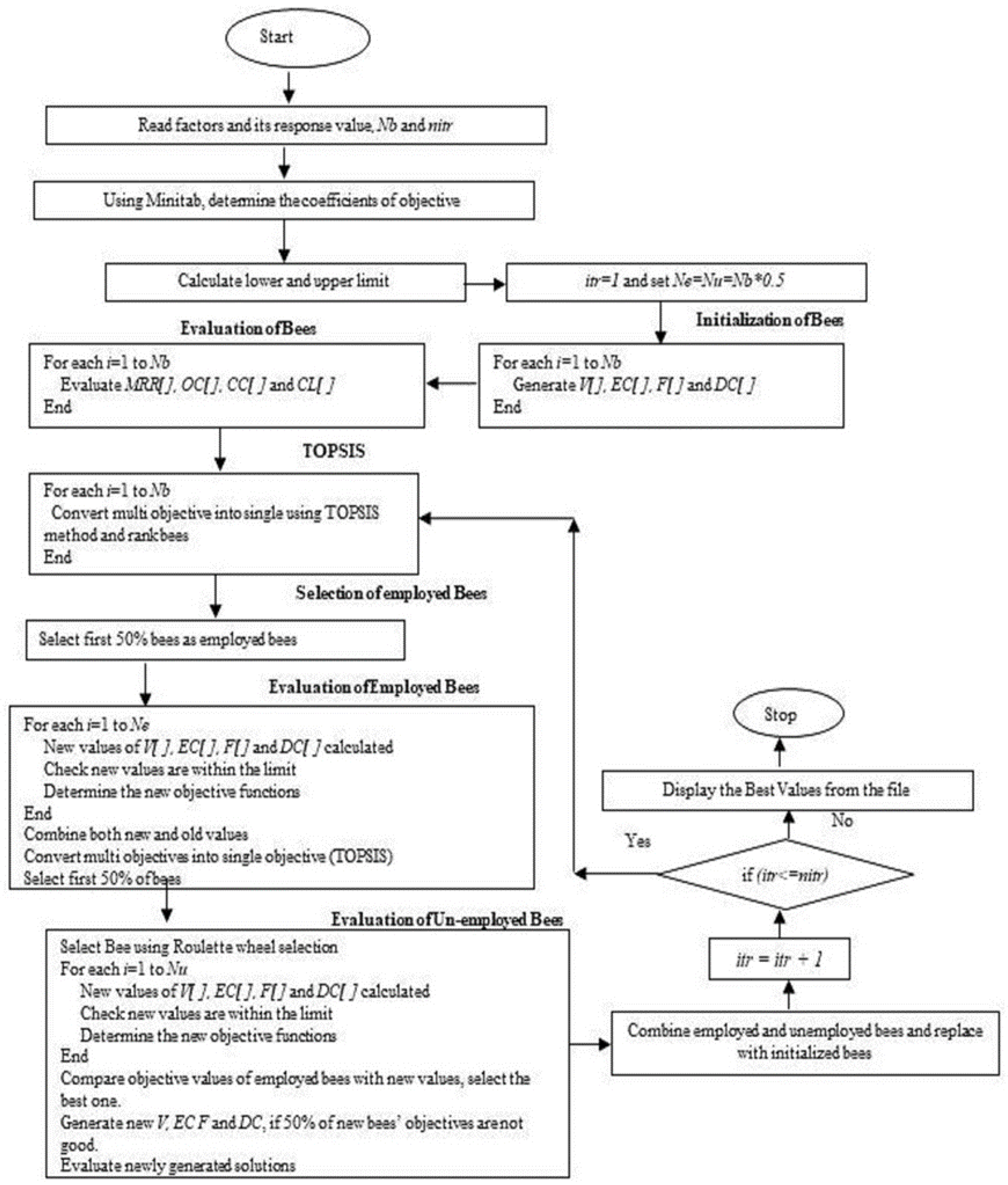
ABC Algorithm
3. Results and Discussion
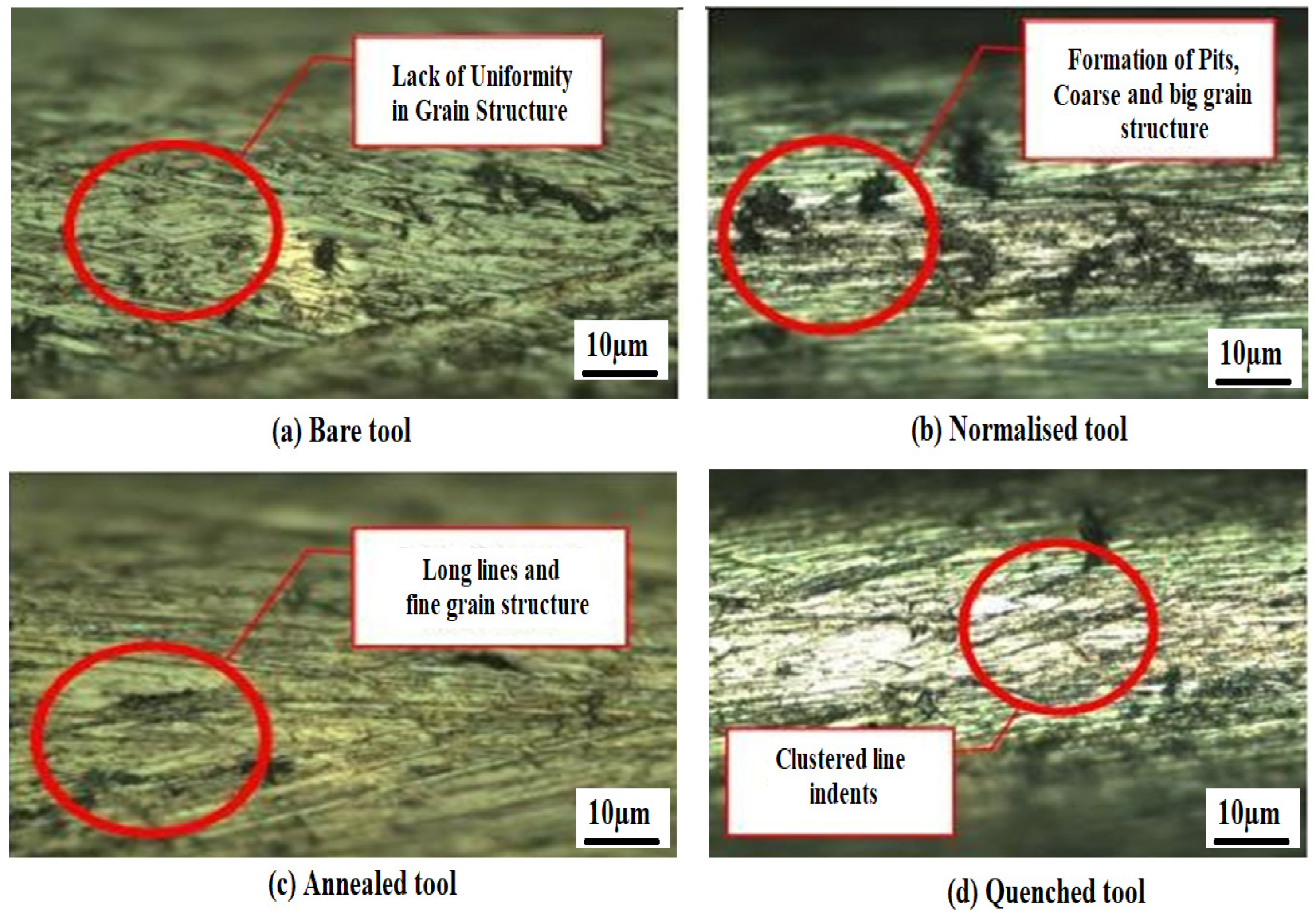
3.1. Influence of Heat Treatment on Copper Tool Electrode
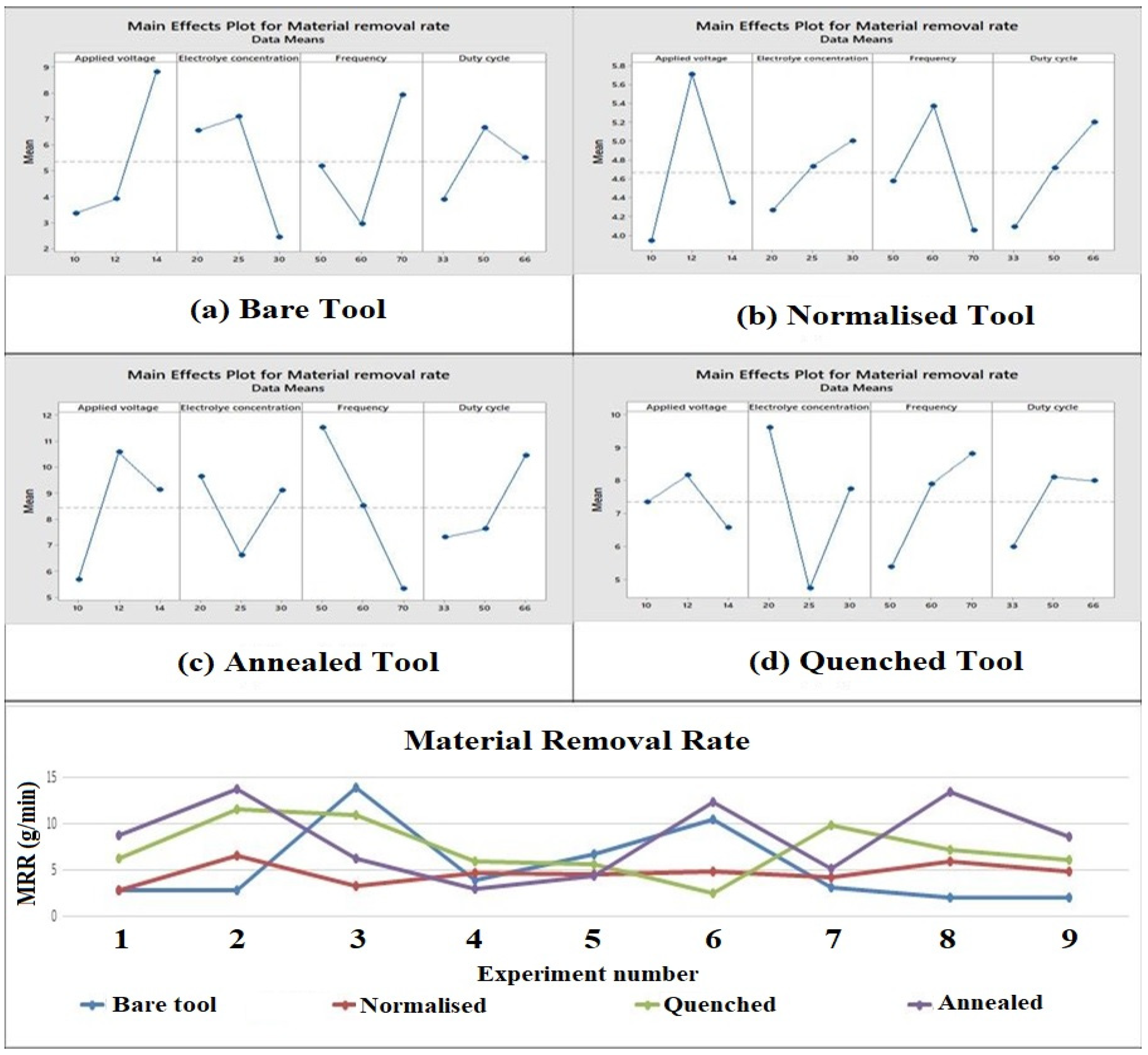
3.2. Influence of Process Parameters and Heat-Treated Tool Electrode on MRR
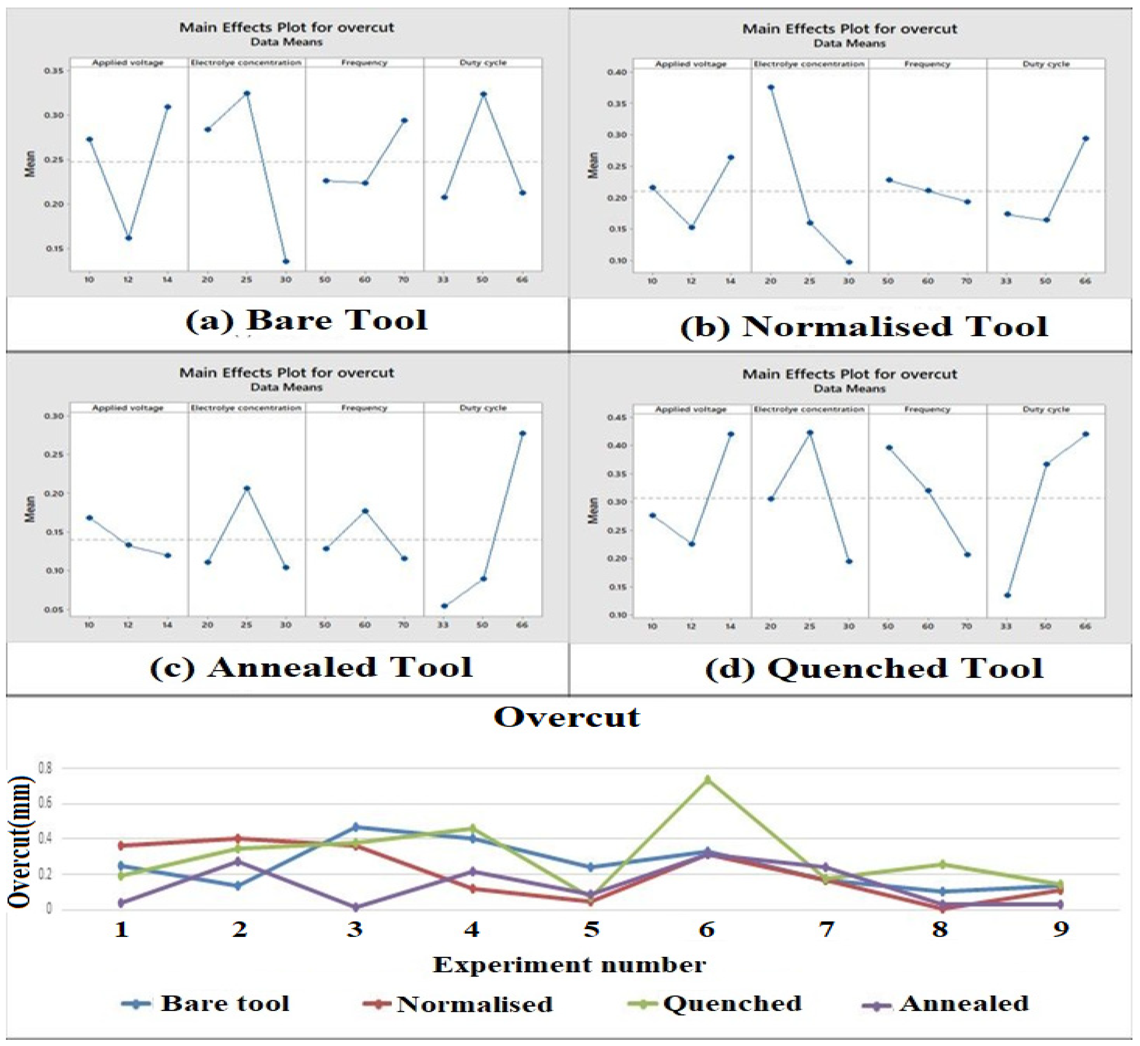
3.3. Influence of Process Parameters and Heat-Treated Tool Electrode on Overcut
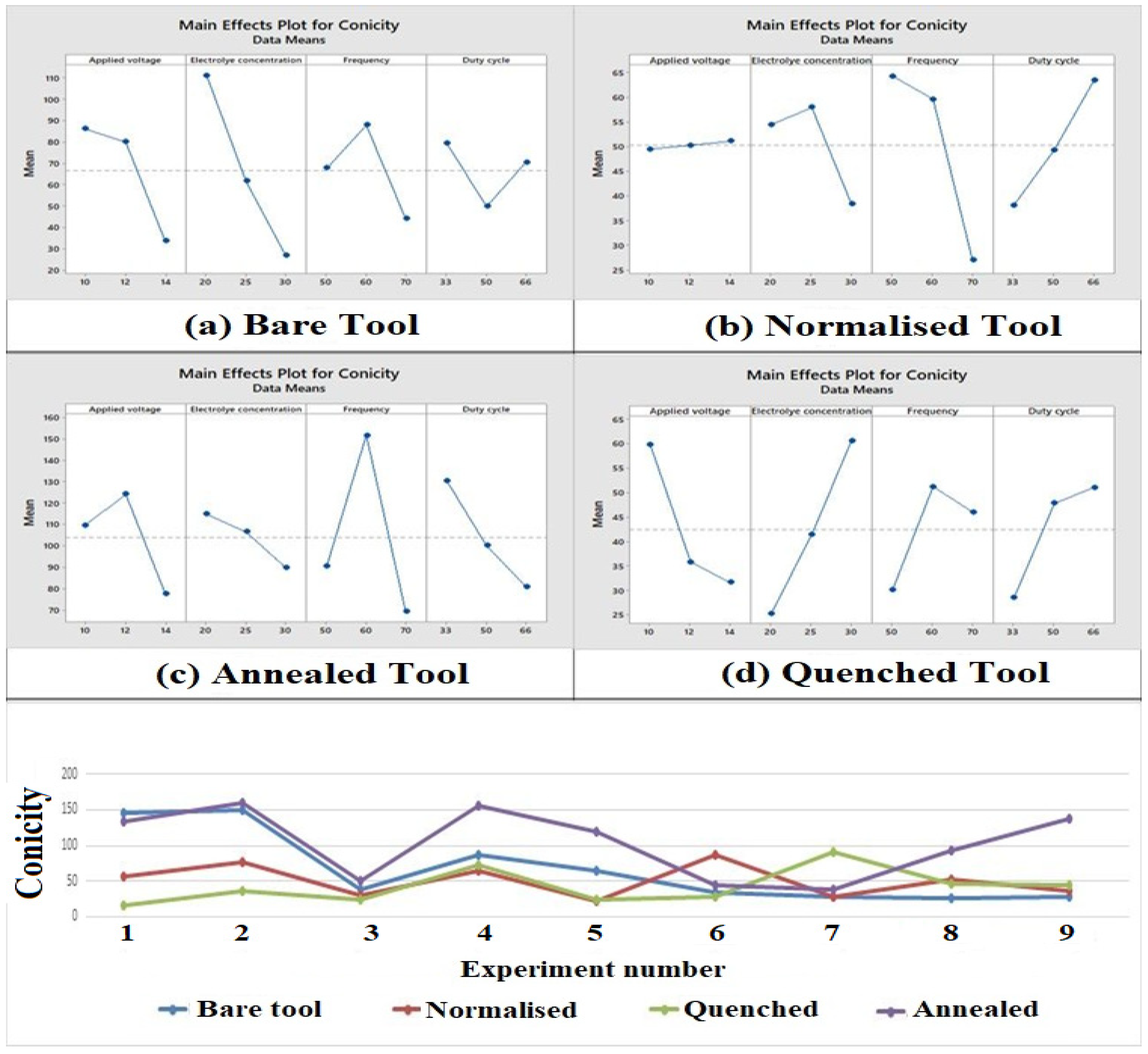
3.4. Influence of Process Parameters and Heat-Treated Tool Electrode on Conicity
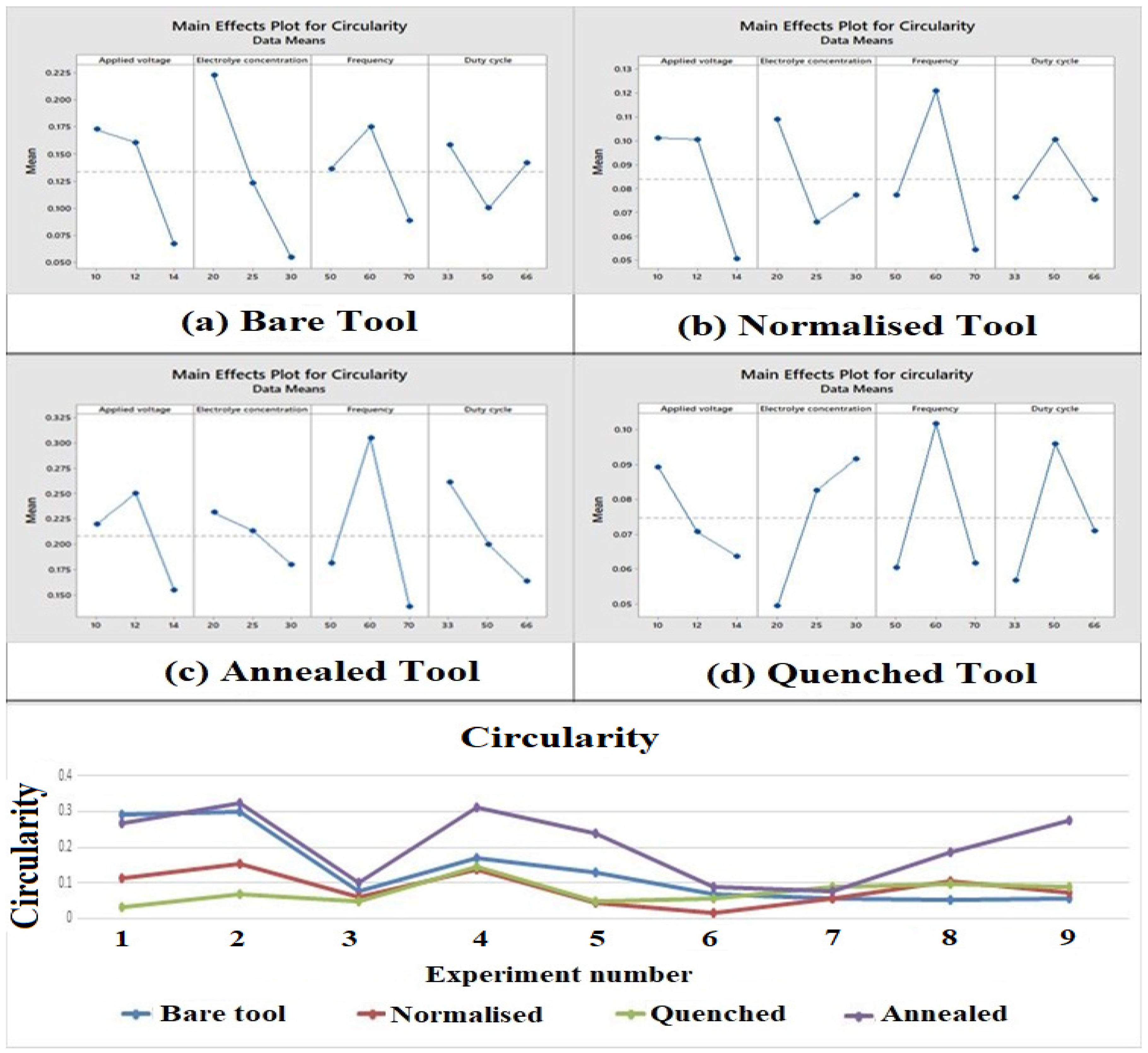
3.5. Influence of Process Parameters and Heat-Treated Tool Electrode on Circularity
4. Analysis of Variance
4.1. ANOVA for MRR
4.2. ANOVA for Overcut
4.3. ANOVA for Conicity
4.4. ANOVA for Circularity
5. Optimum Process Parameters and Their Responses
6. Conclusions
- (i)
- The annealed tool electrode created a higher MRR than the untreated, normalized, and quenched tool electrodes because the annealed tool electrode has a fine grain structure due to the slower rate of cooling and easily dissolves in the electrolyte.
- (ii)
- The annealed tool electrode generated better overcut than the untreated, normalized, and quenched tool electrodes because the annealed tool has a smaller grain structure due to furnace cooling which improves the surface finish of the tool electrode.
- (iii)
- Electrolyte concentration was the most influential parameter for the bare tool as it determines the rate of ionization due to the presence of free ions in the electrolyte.
- (iv)
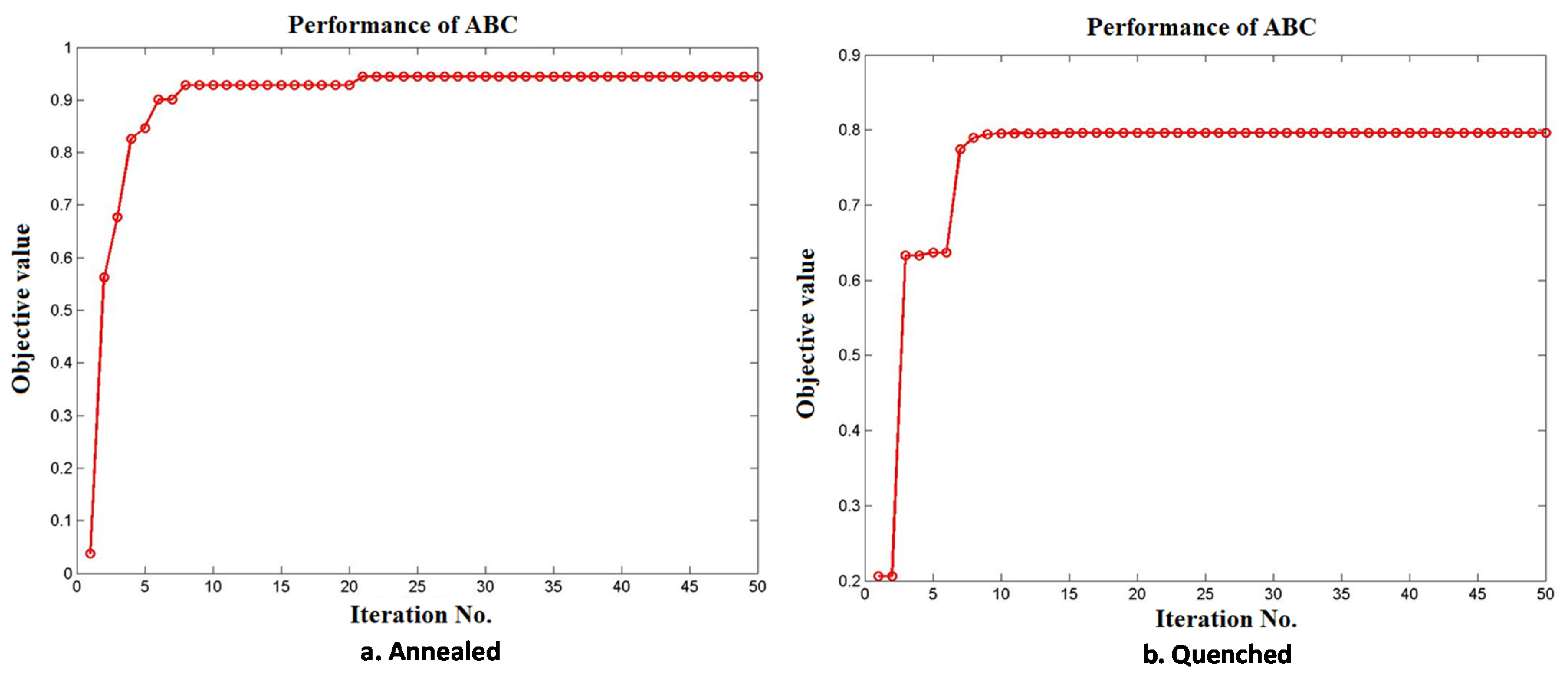
- The optimum combination of input process parameters found using TOPSIS and the ABC algorithm for the EMM process are voltage (14 V), electrolyte concentration (30 g/L), frequency (60 Hz), and duty cycle (33%) for the annealed tool electrode and voltage (14 V), electrolyte concentration (20 g/L), frequency (70 Hz), and duty cycle (33%) for the quenched tool electrode.
Author Contributions
Funding
Data Availability Statement
Acknowledgments
Conflicts of Interest
Nomenclature
| rvj | jth Response value |
| j | Index for response value |
| C0, C1, C2, C3 and C4 | Coefficients of regression equation |
| SST | Sum square total |
| Oij | ith bee’s jth response value |
| i | Index for bee |
| Nij | Normalized value of ith bee’s jth response |
| Aij | Performance value of ith bee’s jth response |
| Wj | Weight of jth response |
| Pj | Positive ideal solution of jth response |
| Mj | Negative ideal solution of jth response |
| SPi | Positive ideal separation value of ith bee |
| SMi | Negative ideal separation value of ith bee |
| OVi | Relative closeness value of ith bee |
| B.No. | Bee number |
| EBNo. | Employed bee number |
| UBNo. | Unemployed bee number |
| nb | Number of bees |
| Pri | Probability of ith bee |
| CPri | Cumulative probability of ith bee |
Appendix A
Appendix A.1. Step 1: Initialization

| B.No. | V | EC | F | DC |
|---|---|---|---|---|
| 1 | 13.26 | 21.58 | 63.11 | 56.30 |
| 2 | 13.62 | 29.71 | 50.71 | 34.05 |
| 3 | 10.51 | 29.57 | 66.98 | 42.14 |
| 4 | 13.65 | 24.85 | 68.68 | 34.52 |
| 5 | 12.53 | 28.00 | 63.57 | 36.21 |
| 6 | 10.39 | 21.42 | 65.15 | 60.17 |
| 7 | 11.11 | 24.22 | 64.86 | 55.93 |
| 8 | 12.19 | 29.16 | 57.84 | 43.46 |
| 9 | 13.83 | 27.92 | 63.11 | 64.36 |
| 10 | 13.86 | 29.59 | 53.42 | 34.14 |
| B.No. | Objectives Matrix–Oij | |||
|---|---|---|---|---|
| MRR | OC | CC | CL | |
| 1 | 9.389 | 0.1698 | 89.0072 | 0.1791 |
| 2 | 11.0122 | 0.0183 | 112.4572 | 0.2241 |
| 3 | 4.0514 | 0.0997 | 108.2449 | 0.216 |
| 4 | 5.7761 | 0.0128 | 104.392 | 0.2082 |
| 5 | 6.3774 | 0.0388 | 108.491 | 0.2163 |
| 6 | 6.6521 | 0.2293 | 104.3681 | 0.2104 |
| 7 | 6.8185 | 0.1902 | 98.2969 | 0.1975 |
| 8 | 8.4807 | 0.0945 | 103.5985 | 0.2069 |
| 9 | 10.3072 | 0.2122 | 56.6152 | 0.1135 |
| 10 | 10.3912 | 0.0143 | 107.8225 | 0.2147 |
Appendix A.2. Step 2: Evaluation
| B.No. | Normalized Value (Nij) | Performance Matrix (Aij) | ||||||
|---|---|---|---|---|---|---|---|---|
| MRR | OC | CC | CL | MRR | OC | CC | CL | |
| 1 | 0.3609 | 0.3962 | 0.28 | 0.2817 | 0.0902 | 0.099 | 0.07 | 0.0704 |
| 2 | 0.4233 | 0.0427 | 0.3537 | 0.3525 | 0.1058 | 0.0107 | 0.0884 | 0.0881 |
| 3 | 0.1557 | 0.2326 | 0.3405 | 0.3398 | 0.0389 | 0.0582 | 0.0851 | 0.0849 |
| 4 | 0.222 | 0.0299 | 0.3284 | 0.3275 | 0.0555 | 0.0075 | 0.0821 | 0.0819 |
| 5 | 0.2451 | 0.0905 | 0.3413 | 0.3402 | 0.0613 | 0.0226 | 0.0853 | 0.0851 |
| 6 | 0.2557 | 0.535 | 0.3283 | 0.331 | 0.0639 | 0.1338 | 0.0821 | 0.0827 |
| 7 | 0.2621 | 0.4438 | 0.3092 | 0.3107 | 0.0655 | 0.1109 | 0.0773 | 0.0777 |
| 8 | 0.326 | 0.2205 | 0.3259 | 0.3255 | 0.0815 | 0.0551 | 0.0815 | 0.0814 |
| 9 | 0.3962 | 0.4951 | 0.1781 | 0.1785 | 0.0991 | 0.1238 | 0.0445 | 0.0446 |
| 10 | 0.3994 | 0.0334 | 0.3392 | 0.3377 | 0.0999 | 0.0083 | 0.0848 | 0.0844 |
| P/M | MRR | OC | CC | CL |
|---|---|---|---|---|
| Pj | 0.1058 | 0.0075 | 0.0445 | 0.0446 |
| Mj | 0.0389 | 0.1338 | 0.0884 | 0.0881 |
| B.No. | SPi | SMi | OVi |
|---|---|---|---|
| 1 | 0.0997 | 0.067 | 0.4019 |
| 2 | 0.0619 | 0.1401 | 0.6936 |
| 3 | 0.1016 | 0.0757 | 0.4271 |
| 4 | 0.073 | 0.1277 | 0.6362 |
| 5 | 0.0742 | 0.1134 | 0.6044 |
| 6 | 0.1434 | 0.0263 | 0.1552 |
| 7 | 0.1204 | 0.0382 | 0.2409 |
| 8 | 0.0747 | 0.0899 | 0.5463 |
| 9 | 0.1165 | 0.0868 | 0.4269 |
| 10 | 0.0569 | 0.1395 | 0.7102 |
Appendix A.3. Step 3: Selection of Employed Bees
| B.No. | V | EC | F | DC | MRR | OC | CC | CL | OV | EBNo. |
|---|---|---|---|---|---|---|---|---|---|---|
| 10 | 13.86 | 29.59 | 53.42 | 34.14 | 10.3912 | 0.0143 | 107.8225 | 0.2147 | 0.7102 | 1′ |
| 2 | 13.62 | 29.71 | 50.71 | 34.05 | 11.0122 | 0.0183 | 112.4572 | 0.2241 | 0.6936 | 2′ |
| 4 | 13.65 | 24.85 | 68.68 | 34.52 | 5.7761 | 0.0128 | 104.392 | 0.2082 | 0.6362 | 3′ |
| 5 | 12.53 | 28.00 | 63.57 | 36.21 | 6.3774 | 0.0388 | 108.491 | 0.2163 | 0.6044 | 4′ |
| 8 | 12.19 | 29.16 | 57.84 | 43.46 | 8.4807 | 0.0945 | 103.5985 | 0.2069 | 0.5463 | 5′ |
Appendix A.4. Step 4: Searching of New Food by Employed Bees
| EBNo.(i) | Rij | ||||
|---|---|---|---|---|---|
| V | EC | F | DC | REBNo.(k) | |
| 1′ | −0.1225 | −0.0205 | −0.4479 | −0.0033 | 4′ |
| 2′ | −0.2369 | −0.1088 | 0.3594 | 0.9195 | 5′ |
| 3′ | 0.531 | 0.2926 | 0.3102 | −0.3192 | 1′ |
| 4′ | 0.5904 | 0.4187 | −0.6748 | 0.1705 | 5′ |
| 5′ | −0.6263 | 0.5094 | −0.762 | −0.5524 | 2′ |
| NEBNo. | New Parameter Value by Employed Bees | New Objective Values | ||||||
|---|---|---|---|---|---|---|---|---|
| nV | nEC | nF | nDC | nMRR | nOC | nCC | nCL | |
| n1 | 13.70 | 29.56 | 57.97 | 34.14 | 10.3912 | 0.0143 | 107.8225 | 0.2147 |
| n2 | 13.28 | 29.65 | 60.94 | 37.57 | 11.0122 | 0.0183 | 112.4572 | 0.2241 |
| n3 | 13.54 | 23.47 | 55.15 | 34.40 | 5.7761 | 0.0128 | 104.392 | 0.2082 |
| n4 | 12.73 | 27.52 | 59.71 | 34.97 | 6.3774 | 0.0388 | 108.491 | 0.2163 |
| n5 | 13.09 | 28.88 | 52.41 | 38.26 | 8.4807 | 0.0945 | 103.5985 | 0.2069 |
| B.No. | V | EC | F | DC | MRR | OC | CC | CL | OV |
|---|---|---|---|---|---|---|---|---|---|
| 1′ | 13.86 | 29.59 | 53.42 | 34.14 | 10.3912 | 0.0143 | 107.8225 | 0.2147 | 0.9362 |
| 2′ | 13.62 | 29.71 | 50.71 | 34.05 | 11.0122 | 0.0183 | 112.4572 | 0.2241 | 0.899 |
| 3′ | 13.65 | 24.85 | 68.68 | 34.52 | 5.7761 | 0.0128 | 104.392 | 0.2082 | 0.7696 |
| 4′ | 12.53 | 28.00 | 63.57 | 36.21 | 6.3774 | 0.0388 | 108.491 | 0.2163 | 0.6226 |
| 5′ | 12.19 | 29.16 | 57.84 | 43.46 | 8.4807 | 0.0945 | 103.5985 | 0.2069 | 0.1669 |
| n1 | 13.70 | 29.56 | 57.97 | 34.14 | 8.8443 | 0.0133 | 104.3467 | 0.2077 | 0.8875 |
| n2 | 13.28 | 29.65 | 60.94 | 37.57 | 7.8853 | 0.0393 | 99.1354 | 0.1973 | 0.6552 |
| n3 | 13.54 | 23.47 | 55.15 | 34.40 | 9.9347 | 0.0232 | 123.3294 | 0.2468 | 0.8084 |
| n4 | 12.73 | 27.52 | 59.71 | 34.97 | 7.6584 | 0.0309 | 114.0552 | 0.2276 | 0.7182 |
| n5 | 13.09 | 28.88 | 52.41 | 38.26 | 10.4647 | 0.0525 | 110.6841 | 0.2209 | 0.543 |
| B.No. | V | EC | F | DC | MRR | OC | CC | CL | OVi | OEBNo. |
|---|---|---|---|---|---|---|---|---|---|---|
| 1′ | 13.86 | 29.59 | 53.42 | 34.14 | 10.3912 | 0.0143 | 107.8225 | 0.2147 | 0.9362 | 1″ |
| 2′ | 13.62 | 29.71 | 50.71 | 34.05 | 11.0122 | 0.0183 | 112.4572 | 0.2241 | 0.899 | 2″ |
| n1 | 13.70 | 29.56 | 57.97 | 34.14 | 8.8443 | 0.0133 | 104.3467 | 0.2077 | 0.8875 | 3″ |
| n3 | 13.54 | 23.47 | 55.15 | 34.40 | 9.9347 | 0.0232 | 123.3294 | 0.2468 | 0.8084 | 4″ |
| 3′ | 13.65 | 24.85 | 68.68 | 34.52 | 5.7761 | 0.0128 | 104.392 | 0.2082 | 0.7696 | 5″ |
Appendix A.5. Step 5: Searching of New Food by Unemployed Bees
| OEBNo. | Pr | CP | Rno | SOEBNo. | UBNo. |
|---|---|---|---|---|---|
| 1″ | 0.2177 | 0.2177 | 0.8143 | 4″ | u1 |
| 2″ | 0.209 | 0.4267 | 0.2435 | 2″ | u2 |
| 3″ | 0.2064 | 0.6331 | 0.9293 | 5″ | u3 |
| 4″ | 0.188 | 0.8211 | 0.35 | 2″ | u4 |
| 5″ | 0.1789 | 1 | 0.1966 | 1″ | u5 |
| UBNo. | V | EC | F | DC | MRR | OC | CC | CL |
|---|---|---|---|---|---|---|---|---|
| u1 | 13.54 | 23.47 | 55.15 | 34.40 | 9.9347 | 0.0232 | 123.3294 | 0.2468 |
| u2 | 13.62 | 29.71 | 50.71 | 34.05 | 11.0122 | 0.0183 | 112.4572 | 0.2241 |
| u3 | 13.65 | 24.85 | 68.68 | 34.52 | 5.7761 | 0.0128 | 104.392 | 0.2082 |
| u4 | 13.62 | 29.71 | 50.71 | 34.05 | 11.0122 | 0.0183 | 112.4572 | 0.2241 |
| u5 | 13.86 | 29.59 | 53.42 | 34.14 | 10.3912 | 0.0143 | 107.8225 | 0.2147 |
| UBNo. | Rij | RUBNo(k) | |||
|---|---|---|---|---|---|
| V | EC | F | DC | ||
| u1 | −0.4978 | 0.1705 | 0.5075 | 0.0616 | u3 |
| u2 | 0.2321 | 0.0994 | −0.2391 | 0.5583 | u1 |
| u3 | −0.0534 | 0.8344 | 0.1356 | 0.868 | u2 |
| u4 | −0.2967 | −0.4283 | −0.8483 | −0.7402 | u1 |
| u5 | 0.6617 | 0.5144 | −0.8921 | 0.1376 | u4 |
| NUBNo. | nV | nEC | nF | nDC | nMRR | nOC | nCC | nCL |
|---|---|---|---|---|---|---|---|---|
| nu1 | 13.60 | 23.23 | 56.22 | 34.39 | 9.6633 | 0.0219 | 122.3431 | 0.2448 |
| nu2 | 13.64 | 25.29 | 51.77 | 33.86 | 10.9167 | 0.0193 | 122.448 | 0.2448 |
| nu3 | 13.65 | 20.81 | 53.31 | 34.93 | 10.7876 | 0.0287 | 130.2479 | 0.2611 |
| nu4 | 13.60 | 27.03 | 54.48 | 34.31 | 9.9926 | 0.0198 | 114.8823 | 0.2293 |
| nu5 | 12.99 | 29.54 | 51.01 | 34.15 | 10.3917 | 0.0265 | 117.4701 | 0.2343 |
| UBNo. | NUBNo. | Cnt | V | EC | F | DC | MRR | OC | CC | CL | ||
|---|---|---|---|---|---|---|---|---|---|---|---|---|
| B.No. | OV | B.No. | OV | |||||||||
| u1 | 0.668 | nu1 | 0.332 | |||||||||
| u2 | 0 | nu2 | 1 | 1 | ||||||||
| u3 | 0.4261 | nu3 | 0.5739 | 2 | ||||||||
| u4 | 0 | nu4 | 1 | 3 | 12.41 | 22.63 | 63.08 | 55.7441 | 8.5554 | 0.1756 | 94.066 | 0.1892 |
| u5 | 0.0006 | nu5 | 0.9994 | 4 | 11.80 | 20.84 | 54.58 | 63.1401 | 11.4591 | 0.2395 | 101.3516 | 0.2047 |
Appendix A.6. Step 6: Replacement of Initial Solution of Bees
| OUBNo. | V | EC | F | DC | MRR | OC | CC | CL |
|---|---|---|---|---|---|---|---|---|
| 1‴ | 13.54 | 23.47 | 55.15 | 34.40 | 9.9347 | 0.0232 | 123.3294 | 0.2468 |
| 2‴ | 13.64 | 25.29 | 51.77 | 33.86 | 10.9167 | 0.0193 | 122.448 | 0.2448 |
| 3‴ | 13.65 | 20.81 | 53.31 | 34.93 | 10.7876 | 0.0287 | 130.2479 | 0.2611 |
| 4‴ | 12.41 | 22.63 | 63.08 | 55.7441 | 8.5554 | 0.1756 | 94.066 | 0.1892 |
| 5‴ | 11.80 | 20.84 | 54.58 | 63.1401 | 11.4591 | 0.2395 | 101.3516 | 0.2047 |
| B.No. | V | EC | F | DC | MRR | OC | CC | CL | OV |
|---|---|---|---|---|---|---|---|---|---|
| 1″ | 13.86 | 29.59 | 53.42 | 34.14 | 10.3912 | 0.0143 | 107.8225 | 0.2147 | 0.9995 |
| 2″ | 13.62 | 29.71 | 50.71 | 34.05 | 11.0122 | 0.0183 | 112.4572 | 0.2241 | 0.9986 |
| 3″ | 13.70 | 29.56 | 57.97 | 34.14 | 8.8443 | 0.0133 | 104.3467 | 0.2077 | 0.9998 |
| 4″ | 13.54 | 23.47 | 55.15 | 34.40 | 9.9347 | 0.0232 | 123.3294 | 0.2468 | 0.9954 |
| 5″ | 13.65 | 24.85 | 68.68 | 34.52 | 5.7761 | 0.0128 | 104.392 | 0.2082 | 0.9998 |
| 1‴ | 13.54 | 23.47 | 55.15 | 34.40 | 9.9347 | 0.0232 | 123.3294 | 0.2468 | 0.9954 |
| 2‴ | 13.64 | 25.29 | 51.77 | 33.86 | 10.9167 | 0.0193 | 122.448 | 0.2448 | 0.9971 |
| 3‴ | 13.65 | 20.81 | 53.31 | 34.93 | 10.7876 | 0.0287 | 130.2479 | 0.2611 | 0.9907 |
| 4‴ | 12.4079 | 22.6297 | 63.0816 | 55.7441 | 8.5554 | 0.1756 | 94.066 | 0.1892 | 0.1382 |
| 5‴ | 11.8022 | 20.8382 | 54.5795 | 63.1401 | 11.4591 | 0.2395 | 101.3516 | 0.2047 | 0.002 |
Appendix A.7. Step 7: Stopping Criteria
References
- De Silva, A.K.M.; Atlena, H.S.J.; McGeough, J.A. Precision ECM by Process Characteristic Modelling. CIRP Ann. 2000, 49, 151–155. [Google Scholar] [CrossRef]
- Bhattacharryya, B.; Mitra, S.; Boro, A.K. Electrochemical machining: New possibilities for micromachining. Robot. Comput.-Integr. Manuf. 2002, 18, 283–289. [Google Scholar] [CrossRef]
- Bhattacharyya, B.; Munda, J. Experimental investigation into electrochemical micromachining (EMM) process. J. Mater. Processing Technol. 2003, 140, 287–291. [Google Scholar] [CrossRef]
- Bhattacharyya, B.; Malapati, M.; Munda, J. Experimental study on electrochemical micromachining (EMM) process. J. Mater. Processing Technol 2005, 169, 485–492. [Google Scholar] [CrossRef]
- Babar, P.D.; Jadhav, B.R. Experimental Study on Parametric Optimization of Titanium based Alloy (Ti-6Al-4V) in Electrochemical Machining, Process. Int. J. Innov. Eng. Technol. 2013, 2, 171–175. [Google Scholar]
- Geethapriyan, T.; Muthuramalingam, T.; Vasanth, S.; Thavamani, J.; Srinivasan, V.H. Influence of Nanoparticles-Suspended Electrolyte on Machinability of Stainless Steel 430 Using Electrochemical Micro- machining Process. Adv. Manuf. Processes 2019, 912, 433–440. [Google Scholar]
- Geethapriyan, T.; Manoj Samson, R.; Thavamani, J.; Arun Raj, A.C.; Pulagam, B.R. Experimental Investigation of Electrochemical Micro-machining Process Parameters on Stainless Steel 316 Using Sodium Chloride Electrolyte. Adv. Manuf. Processes 2019, 471–480. [Google Scholar]
- Geethapriyan, T.; Kalaichelvan, K.; Muthuramalingam, T. Multi Performance Optimization of Electrochemical Micro-Machining Process Surface Related Parameters on Machining Inconel 718 using Taguchi-grey relational analysis. La Metall. Ital. 2016, 4, 13–19. [Google Scholar]
- Das, A.K.; Saha, P. Experimental investigation on micro-electrochemical sinking operation for fabrication of micro-holes. J. Braz. Soc. Mech. Sci. Eng. 2015, 37, 657–663. [Google Scholar] [CrossRef]
- Ahn, S.H.; Ryu, S.H.; Choi, D.K.; Chu, C.N. Electro-chemical micro drilling using ultra short pulses. Prec. Eng. 2004, 28, 129–134. [Google Scholar] [CrossRef]
- Wielage, B.; Mäder, T.; Fürderer, B.; Nestler, D.; Reinecke, H. Carbon fibres used as electrode tools for micro-electrochemical machining. In Proceedings of the 17th International Conference on Composite Materials, Edinburgh, UK, 27–31 July 2019. [Google Scholar]
- Zhu, D.; Xu, H.Y. Improvement of electrochemical machining accuracy by using dual pole tool. J. Mater. Processing Technol. 2002, 129, 15–18. [Google Scholar] [CrossRef]
- Thanigaivelan, R.; Arunachalam, R.M. Experimental study on the influence of tool electrode tip shape on electrochemical micromachining of 304 stainless steel. Mater. Manuf. Processes 2010, 25, 1181–1185. [Google Scholar] [CrossRef]
- Geethapriyan, T.; Kalaichelvan, K.; Muthuramalingam, T. Influence of coated tool electrode on drilling Inconel Alloy 718 in Electrochemical micro machining. Procedia CIRP 2016, 46, 127–130. [Google Scholar] [CrossRef]
- Tsui, H.P.; Hung, J.C.; You, J.C.; Yan, B.H. Improvement of electrochemical microdrilling accuracy using helical tool. Mater. Manuf. Processes 2008, 23, 499–505. [Google Scholar] [CrossRef]
- Zhang, Z.; Zhu, D.; Qu, N.; Wang, M. Theoretical and experimental investigation on electrochemical micro machining. Microsyst. Technol. 2007, 13, 607–612. [Google Scholar] [CrossRef]
- Park, B.J.; Kim, B.H.; Chu, C.N. The Effects of Tool Electrode Size on Characteristics of Micro Electrochemical Machining. CIRP Ann. 2006, 55, 197–200. Available online: https://www.sciencedirect.com/science/journal/00078506/55/1 (accessed on 30 June 2007). [CrossRef]
- Yang, I.; Park, M.S.; Chu, C.N. Micro ECM with Ultrasonic Vibrations Using a Semi-cylindrical Tool. Int. J. Precis. Eng. Manuf. 2009, 10, 5–10. [Google Scholar] [CrossRef]
- Geethapriyan, T.; Lakshmanan, P.; Prakash, M.; Mohammed Iqbal, U.; Suraj, S. Influenceof Tool Electrodes on Machinability of Stainless Steel 420 Using Electrochemical Micromachining Process. Adv. Manuf. Processes 2019, 895, 441–456. [Google Scholar]
- Thangaraj, M.; Ahmadein, M.; Alsaleh, N.A.; Elsheikh, A.H. Optimization of Abrasive Water Jet Machining of SiC Reinforced Aluminum Alloy Based Metal Matrix Composites Using Taguchi–DEAR Technique. Materials 2021, 14, 6250. [Google Scholar] [CrossRef]
- Thangaraj, M.; Moiduddin, K.; Akash, R.; Krishnan, S.; Mian, S.H.; Ameen, W.; Alkhalefah, H. Influence of process parameters on dimensional accuracy of machined Titanium (Ti-6Al-4V) alloy in Laser Beam Machining Process. Opt. Laser Technol. 2020, 132, 106494. [Google Scholar]
- Muthuramalingam, T.; Ramamurthy, A.; Moiduddin, K.; Alkindi, M.; Ramalingam, S.; Alghamdi, O. Enhancing the Surface Quality of Micro Titanium Alloy Specimen in WEDM Process by Adopting TGRA-Based Optimization. Materials 2020, 13, 1440. [Google Scholar]
- Muthuramalingam, T.; Akash, R.; Krishnan, S.; Phan, N.H.; Pi, V.N.; Elsheikh, A.H. Surface quality measures analysis and optimization on machining titanium alloy using CO2 based Laser beam drilling process. J. Manuf. Processes 2021, 62, 1–6. [Google Scholar] [CrossRef]
- Phan, N.H.; Thangaraj, M. Multi criteria decision making of vibration assisted EDM process parameters on machining silicon steel using Taguchi-dear methodology. Silicon 2021, 13, 1879–1885. [Google Scholar] [CrossRef]
- Phan, N.H.; Van Dong, P.; Dung, H.T.; Van Thien, N.; Muthuramalingam, T.; Shirguppikar, S.; Tam, N.C.; Ly, N.T. Multi-object optimization of EDM by Taguchi-dear method using AlCrNi coated electrode. Int. J. Adv. Manuf. Technol. 2021, 116, 1429–1435. [Google Scholar] [CrossRef]
- Schuster, R.; Krirchner, V.; Allongue, P.; Ertl, G. Electrochemical micro machining. Science 2000, 289, 98–101. [Google Scholar] [CrossRef] [PubMed]
- Masuzawa, T. State of the art of micromachining. CIRP Ann. 2000, 49, 473–488. [Google Scholar] [CrossRef]
- Forster, R.; Schoth, A.; Menz, W. Micro-ECM for production of microsystems with a high aspect ratio. Micros. Technol. 2005, 11, 246–249. [Google Scholar] [CrossRef]
- Siva, M.; Karthikeyan, A.; Muthukumar, P.; Babu, B.; Ragoth Singh, R.; Surendar, S. Experimental analysis of aluminum metal matrix composites using electrochemical micro machining. Int. J. Eng. Res. Technol. 2014, 3, 1331–1335. [Google Scholar]
- Ranjithkumar, A.; Malayalamurthy, R. Investigation on micro ECM Compatibility of Al6082Metal matrix composite material. TAGA J. 2018, 14, 2262–2273. [Google Scholar]
- Singh, S.; Singh, R. Some investigation on surface roughness of aluminium metal composite primed by fused deposition modeling-assisted investment casting using reinforced filament. J. Braz. Soc. Mech. Sci. Eng. 2017, 39, 471–479. [Google Scholar] [CrossRef]
- Muthuramalingam, T.; Vasanth, S.; Vinothkumar, P.; Geethapriyan, T.; Rabik, M.M. Multi Criteria Decision Making of Abrasive Flow Oriented Process Parameters in Abrasive Water Jet Machining Using Taguchi–DEAR Methodology. Silicon 2018, 10, 2015–2021. [Google Scholar] [CrossRef]
- Geethapriyan, T.; Muthuramalingam, T.; Moiduddin, K.; Mian, S.M.; Alkhalefah, H.; Umer, U. Performance Analysis of Electrochemical Micro Machining of Titanium (Ti-6Al-4V) Alloy under Different Electrolytes Concentrations. Materials 2021, 11, 247. [Google Scholar]
- Leokumar, S.P.; Jerald, J.; Kumanan, S.; Prabakaran, R. A Review on current aspects in tool based micromachining process. Mater. Manuf. Processes 2014, 1291–1337. [Google Scholar] [CrossRef]
- Das, M.K.; Kumar, K.; Barman, T.K.; Sahoo, P. Investigation on electrochemical machining of EN31 steel for optimization of MRR and Surface roughness using Artificial Bee Colony Algorithm. Procedia Eng. 2014, 97, 1587–1596. [Google Scholar] [CrossRef][Green Version]
- Samanta, S.; Chakraborty, S. Parametric optimization of some non-traditional machining process using artificial bee colony algorithm. Eng. Appl. Artif. Intell. 2011, 24, 946–957. [Google Scholar] [CrossRef]
- Selvaraj, K.; Senniangiri, N.; Aravindkumar, V.C.; Dineshkumar, S.; Dilipkumar, S. Investigation of microhole process parameters of copper alloy and stainless steel using micro ECM. Int. J. Innov. Res. Sci. Technol. 2017, 9–18. [Google Scholar]
- Ahmed, N.; Rafaqat, M.; Pervaiz, S.; Umer, U.; Alkhalefa, H.; Shar, M.A.; Mian, S.H. Controlling the material removal and roughness of Inconel 718 in laser machining. Mater. Manuf. Processes 2019, 34, 1169–1181. [Google Scholar] [CrossRef]
- Eldrup, M.; Singh, B.N. Influence of compositon, heat treatment and neutron irradiation on the electrical conductivity of copper alloys. J. Nucl. Mater. 1998, 258, 1022–1027. [Google Scholar] [CrossRef]
- Davis, J.R. (Ed.) Copper and Copper Alloys; ASM International: Materials Park, OH, USA, 2001; pp. 1–652. [Google Scholar]
- Geethapiriyan, T.; Muthuramalingam, T.; Kalaichelvan, K. Influence of process parameters on machinability of Inconel 718 by electrical micromachining process using Topsis technique. Arab. J. Sci. Eng. 2019, 44, 7945–7955. [Google Scholar] [CrossRef]
- Liu, S.; Geethapriyan, T.; Muthuramalingam, T.; Shanmugam, R.; Ramoni, M. Influence of heat-treated Cu–Be electrode on machining accuracy in ECMM with Monel 400 alloy. Arch. Civ. Mech. Eng. 2022, 22, 1–5. [Google Scholar] [CrossRef]
- Pillai, H.P.; Chinnakulanthai Sampath, S.; Elumalai, R.; Hariharan, S.; Natarajan, Y. Influence of process parameters on electrochemical micromachining of NIMONIC 75 alloy. In Proceedings of the ASME International Mechanical Engineering Congress and Exposition, Tampa, FL, USA, 3–9 November 2017; Volume 2, pp. 1–8. [Google Scholar]
- Maniraj, S.; Thanigaivelan, R. Effect of electrode heating on performance of electrochemical micromachining. Mater. Manuf. Processes 2019, 1–8. [Google Scholar] [CrossRef]
- Pradeep, N.; ShanmugaSundaram, K.; Pradeepkumar, M. Multi-response optimization of electrochemical micromachining parameters for SS304 using polymer graphite electrode with NaNO3 electrolyte based on TOPSIS technique. J. Braz. Soc. Mech. Sci. Eng. 2019, 41, 323. [Google Scholar] [CrossRef]
- Geethapriyan, T.; Kalaichelvan, K.; Muthuramalingam, T.; Rajadurai, A. Performance Analysis of Process Parameters on Machining α-β Titanium Alloy in Electrochemical Micromachining Process. Proc. Inst. Mech. Eng. Part B J. Eng. Manuf. 2016, 1–13. [Google Scholar] [CrossRef]
- Senthilkumar, C.; Ganesan, G.; Karthikeyan, R. Optimization of ECMM process parameters using NSGA-II. J. Miner. Mater. Charact. Eng. 2012, 11, 931–937. [Google Scholar]
- Das, M.K.; Kumar, K.; Barman, T.K.; Sahoo, P. Optimization of surface roughness and MRR in electrochemical machining of EN31 Tool Steel using Grey-Taguchi approach. Procedia Mater. Sci. 2014, 6, 729–740. [Google Scholar] [CrossRef]
- Puertas, I.; Luis, C.J. A Study of optimization of machinng parameters of electrical discharge machining of Boron carbide. Mater. Manuf. Processes 2004, 19, 1041–1070. [Google Scholar] [CrossRef]
- Huo, J.; Liu, S.; Wang, Y.; Muthuramalingam, T.; Pi, V.N. Influence of process factors on surface measures on electrical discharge machined stainless steel using TOPSIS. Mater. Res. Express. 2019, 6, 086507. [Google Scholar] [CrossRef]


| Process Parameters | Level I | Level II | Level III |
|---|---|---|---|
| Voltage (V) | 10 | 12 | 14 |
| Concentration of Electrolyte (g/L) | 20 | 25 | 30 |
| Frequency (Hz) | 50 | 60 | 70 |
| Duty Factor (%) | 33 | 50 | 66 |
| E.No. | V | EC | F | DC | MRR | OC | CC | CL |
|---|---|---|---|---|---|---|---|---|
| 1 | 10 | 20 | 50 | 33 | 8.767 | 0.0405 | 134.0 | 0.269 |
| 2 | 12 | 20 | 60 | 66 | 13.804 | 0.2770 | 160.0 | 0.325 |
| 3 | 14 | 20 | 70 | 50 | 6.354 | 0.0145 | 50.5 | 0.100 |
| 4 | 10 | 25 | 60 | 50 | 3.076 | 0.2205 | 156.5 | 0.313 |
| 5 | 12 | 25 | 70 | 33 | 4.444 | 0.0875 | 119.0 | 0.238 |
| 6 | 14 | 25 | 50 | 66 | 12.345 | 0.3105 | 44.5 | 0.089 |
| 7 | 10 | 30 | 70 | 66 | 5.181 | 0.2430 | 38.5 | 0.077 |
| 8 | 12 | 30 | 50 | 50 | 13.453 | 0.0335 | 93.5 | 0.187 |
| 9 | 14 | 30 | 60 | 33 | 8.695 | 0.0335 | 138.0 | 0.276 |
| rvj | Coefficients | ||||
|---|---|---|---|---|---|
| C0 | C1 | C2 | C3 | C4 | |
| MRR | 13.3151 | 0.8642 | −0.0532 | −0.3098 | 0.0944 |
| OC | 0.0102 | −0.0121 | −0.0007 | −0.0007 | 0.0067 |
| CC | 400.31 | −8 | −2.4833 | −1.0667 | −1.4979 |
| CL | 0.8074 | −0.0162 | −0.0051 | −0.0022 | −0.003 |
| E.No. | V | EC | F | DC | MRR | OC | CC | CL |
|---|---|---|---|---|---|---|---|---|
| 1 | 10 | 20 | 50 | 33 | 6.231 | 0.1895 | 16.5 | 0.032 |
| 2 | 12 | 20 | 60 | 66 | 11.5700 | 0.3475 | 36.0 | 0.069 |
| 3 | 14 | 20 | 70 | 50 | 11.020 | 0.3765 | 23.5 | 0.047 |
| 4 | 10 | 25 | 60 | 50 | 6.000 | 0.4625 | 73.0 | 0.146 |
| 5 | 12 | 25 | 70 | 33 | 5.600 | 0.0675 | 24.5 | 0.048 |
| 6 | 14 | 25 | 50 | 66 | 2.612 | 0.7355 | 27.0 | 0.054 |
| 7 | 10 | 30 | 70 | 66 | 9.800 | 0.1745 | 90.0 | 0.090 |
| 8 | 12 | 30 | 50 | 50 | 7.294 | 0.2605 | 47.0 | 0.095 |
| 9 | 14 | 30 | 60 | 33 | 6.122 | 0.1465 | 44.5 | 0.090 |
| rvj | Coefficients | ||||
|---|---|---|---|---|---|
| C0 | C1 | C2 | C3 | C4 | |
| MRR | 0.9682 | −0.1897 | −0.1868 | 0.1714 | 0.0616 |
| OC | 0.2874 | 0.036 | −0.0111 | −0.0094 | 0.0087 |
| CC | −42.5712 | −7.0417 | 3.5167 | 0.7917 | 0.6866 |
| CL | 0.0192 | −0.0064 | 0.0042 | 0.0001 | 0.0005 |
| Limits | V | EC | F | DC |
|---|---|---|---|---|
| Lower | 10 | 20 | 50 | 33 |
| Upper | 14 | 30 | 70 | 66 |
| Parameters | Value |
|---|---|
| No. of Bees (Population Bees) | 30 |
| No. of Employed Bees | 15 (50% of total bees) |
| No. of Unemployed Bees | 15 (50% of total bees) |
| Termination Criteria | 50 iterations |
| Source | DF | Adj SS | Adj MS | F-Value | p-Value | Contribution |
|---|---|---|---|---|---|---|
| Regression | 4 | 90.482 | 22.6205 | 2.35 | 0.214 | |
| Applied voltage | 1 | 17.923 | 17.9228 | 1.86 | 0.244 | 13.89 |
| Electrolyte concentration | 1 | 0.425 | 0.4245 | 0.04 | 0.844 | 0.32 |
| Frequency | 1 | 57.573 | 57.5732 | 5.97 | 0.071 | 44.61 |
| Duty cycle | 1 | 14.561 | 14.5614 | 1.51 | 0.286 | 11.28 |
| Error | 4 | 38.552 | 9.6380 | |||
| Total | 8 | 129.034 |
| Source | DF | Adj SS | Adj MS | F-Value | p-Value | Contribution |
|---|---|---|---|---|---|---|
| Regression | 4 | 0.077419 | 0.019355 | 2.01 | 0.258 | |
| Applied voltage | 1 | 0.003528 | 0.003528 | 0.37 | 0.578 | 3.04 |
| Electrolyte concentration | 1 | 0.000081 | 0.000081 | 0.01 | 0.932 | 0.06 |
| Frequency | 1 | 0.000260 | 0.000260 | 0.03 | 0.878 | 0.22 |
| Duty cycle | 1 | 0.073550 | 0.073550 | 7.62 | 0.051 | 45.91 |
| Error | 4 | 0.038601 | 0.009650 | |||
| Total | 8 | 0.116020 |
| Source | DF | Adj SS | Adj MS | F-Value | p-Value | Contribution |
|---|---|---|---|---|---|---|
| Regression | 4 | 4191.3 | 1047.8 | 6.32 | 0.051 | |
| Applied voltage | 1 | 1190.0 | 1190.0 | 7.18 | 0.055 | 24.56 |
| Electrolyte concentration | 1 | 1855.0 | 1855.0 | 11.19 | 0.029 | 38.28 |
| Frequency | 1 | 376.0 | 376.0 | 2.27 | 0.206 | 7.76 |
| Duty cycle | 1 | 770.2 | 770.2 | 4.65 | 0.097 | 15.89 |
| Error | 4 | 662.9 | 165.7 | |||
| Total | 8 | 4854.2 |
| Source | DF | Adj SS | Adj MS | F-Value | p-Value | Contribution |
|---|---|---|---|---|---|---|
| Regression | 4 | 0.004016 | 0.001004 | 0.70 | 0.629 | |
| Applied voltage | 1 | 0.000988 | 0.000988 | 0.69 | 0.452 | 10.156 |
| Electrolyte concentration | 1 | 0.002688 | 0.002688 | 1.88 | 0.242 | 27.63 |
| Frequency | 1 | 0.000003 | 0.000003 | 0.00 | 0.968 | 0.03 |
| Duty cycle | 1 | 0.000337 | 0.000337 | 0.24 | 0.653 | 3.46 |
| Error | 4 | 0.005713 | 0.001428 | |||
| Total | 8 | 0.009728 |
| Type | V | EC | F | DC | MRR | OC | CC | CL |
|---|---|---|---|---|---|---|---|---|
| Annealed | 13.9947 | 29.9974 | 59.0402 | 33.0503 | 8.64425 | 0.00136 | 101.379 | 0.20152 |
| Quenched | 13.4648 | 20.004 | 66.4348 | 33.0107 | 8.09388 | 0.20939 | 8.21947 | 0.03688 |
| Type | V | EC | F | DC | MRR | OC | CC | CL |
|---|---|---|---|---|---|---|---|---|
| Annealed | 14 | 30 | 60 | 33 | 8.82265 | 0.00122 | 96.582 | 0.18526 |
| Quenched | 14 | 20 | 70 | 33 | 8.42349 | 0.22548 | 7.8254 | 0.05125 |
Publisher’s Note: MDPI stays neutral with regard to jurisdictional claims in published maps and institutional affiliations. |
© 2022 by the authors. Licensee MDPI, Basel, Switzerland. This article is an open access article distributed under the terms and conditions of the Creative Commons Attribution (CC BY) license (https://creativecommons.org/licenses/by/4.0/).
Share and Cite
Thangamani, G.; Thangaraj, M.; Moiduddin, K.; Alkhalefah, H.; Mahalingam, S.; Karmiris-Obratański, P. Multiobjective Optimization of Heat-Treated Copper Tool Electrode on EMM Process Using Artificial Bee Colony (ABC) Algorithm. Materials 2022, 15, 4831. https://doi.org/10.3390/ma15144831
Thangamani G, Thangaraj M, Moiduddin K, Alkhalefah H, Mahalingam S, Karmiris-Obratański P. Multiobjective Optimization of Heat-Treated Copper Tool Electrode on EMM Process Using Artificial Bee Colony (ABC) Algorithm. Materials. 2022; 15(14):4831. https://doi.org/10.3390/ma15144831
Chicago/Turabian StyleThangamani, Geethapriyan, Muthuramalingam Thangaraj, Khaja Moiduddin, Hisham Alkhalefah, Sivakumar Mahalingam, and Panagiotis Karmiris-Obratański. 2022. "Multiobjective Optimization of Heat-Treated Copper Tool Electrode on EMM Process Using Artificial Bee Colony (ABC) Algorithm" Materials 15, no. 14: 4831. https://doi.org/10.3390/ma15144831
APA StyleThangamani, G., Thangaraj, M., Moiduddin, K., Alkhalefah, H., Mahalingam, S., & Karmiris-Obratański, P. (2022). Multiobjective Optimization of Heat-Treated Copper Tool Electrode on EMM Process Using Artificial Bee Colony (ABC) Algorithm. Materials, 15(14), 4831. https://doi.org/10.3390/ma15144831