
The Nature, Causes and Extent of Land cover Changes in Gamtoos River Estuary, Eastern Cape Province, South Africa: 1991–2017


1
Department of GIS & Remote Sensing, University of Fort Hare, Private Bag X314, Alice 5700, South Africa
2
Risk and Vulnerability Science Centre, University of the Free State, Private Bag X13, Phuthaditjhaba 9866, South Africa
*
Author to whom correspondence should be addressed.
Sustainability 2022, 14(13), 7859; https://doi.org/10.3390/su14137859
Submission received: 20 March 2022
/
Revised: 22 April 2022
/
Accepted: 3 May 2022
/
Published: 28 June 2022
Abstract
:Multi-date remotely sensed SPOT images of 1991, 2000, 2009 and 2017 were used to reconstruct changes in land cover in the Gamtoos River Estuary, Eastern Cape province, South Africa. These images were complemented by near-anniversary aerial photographs and Google Earth images that were used as ancillary sources of ground truth. The long-term trend direction of change was determined by calculating percentage changes and performing linear trend analysis. The magnitude of change was established by calculating Sen Slope estimates (SSE) and the influence of climate change on changes in land cover tested by correlating changes in rainfall and different cover types. The greatest and lowest changes were for noncultivated land and surface water (−7.94%, y = −1.2032x + 21.275, SSE = −0.292, and 0.44%, y = −0.4261x + 9.657, SSE = 0.007, respectively). Correlations between rainfall and all cover types were weak and ranged between 0.453816 and −0.643962. Rainfall exhibited a significant decrease (p = 0.0411, σ 0.05; y = −7.175x + 734.55, SSE = −11.130) that was highly correlated with changes in surface water distribution (0.813709, Critical R = 0.805). Overall, the results of this investigation point to the combined influence of climate change and human agency, with the latter tending to play a more prominent role by exerting increasing pressure on the environment’s natural supporting potentials. We therefore urge the scientific community to continue exploring actionable interventions that can be used to enhance the sustainability of this ecosystem and others elsewhere.
1. Introduction
Estuaries are semi-enclosed coastal bodies of water which are connected to the sea either permanently or periodically, with salinities that are different from that of the adjacent open ocean due to freshwater inputs. [1]. They are some the world’s most dynamic aquatic environments [2] and more productive than freshwater and marine ecosystems [3]. Apart from providing ecosystem goods and services ranging from fisheries to recreational opportunities [4,5], they also store genetic resources that can be exploited for human gain [6]. Although their full value is often underestimated [7], they support the livelihoods of local communities by providing more benefits than what most ecosystems can offer [4]. Unfortunately, however, their sustainability is being compromised by inappropriate human resource use practices and climate change [8] with evidence showing that worldwide, they are some of the most threatened natural systems [9]. In South Africa, these ecosystems are under increasing anthropogenic stressors, with nutrient enrichment being reported to be the main cause of their deteriorating water quality [10,11]. Persistent enrichment is a major problem because some of the nutrients persist as ‘legacy nutrients’ even after input has ceased [12,13,14].
Other anthropogenic stressors and impacts include (1) the conversion of land to agriculture and settlement, (2), reduced freshwater inflow from impoundment in dams [15], (3) increased pollution from urban runoff [16], (4) water table elevation from agricultural return flow [17], (5) the contamination of soils from overfertilisation on crop farms and runoff from cattle [18], (6) declining nursery value due to recreational fishing pressure and pollution, (7) freshwater starvation by competing demands that include irrigation agriculture and abstraction for industrial and domestic consumption [19] and (8) hydrological modifications from excessive abstraction and planned diversion [20,21,22]. Although giving detailed explanations of these factors is beyond the scope of this paper, an elaboration of selected examples may help to illustrate how human interventions and inappropriate resource practices are threatening the sustainability of these ecosystems. The conversion of land to agriculture and settlement, for instance, entails the clearing of dryland vegetation and the baring of landscapes. This directly impacts on estuarine ecosystems by modifying inflow from surface runoff, reducing flushing rates and increasing the residence times for different nutrients and pollutants.
The combined effects of these modifications are variable, but they all imply the alteration of seasonal inundation patterns, changes in nutrient dynamics and the distribution of water-tolerant and water-intolerant herbaceous species. In terms of pollution and nutrient overloading, the 840,000 m3 of wastewater disposed into South Africa’s estuaries on a daily basis points to substantial human impact [22]. This leads to nutrient overloading when the system’s assimilative capacity is exceeded. The construction of dams in some of the estuaries’ catchment areas aggravates this situation by reducing freshwater inflows and diverting river water to irrigation and domestic and industrial use. These extractive uses of water further imply reduced mixing of estuarine water and surface runoff and the conversion of estuaries into nutrient sinks.
Climate-change-related stressors include (1) sea-level rise (SLR)-induced loss of estuarine area [23,24,25,26], (2) the alteration of salt marsh zonation, habitat modification, reduced productivity and salinization of terrestrial and estuarine freshwater by seawater [27], (3) the increased frequency of destructive floods [28], (4) the disruption of salinity regimes during periods of prolonged rainfall failures and drought [29] and (5) the loss of biodiversity and eutrophication from the intermittent isolation of estuarine water and reduced connectivity to the sea [30]. These threats explain why climate change has been identified as one of the root causes of persistent decrease in the productivity of estuaries [31].
In South Africa, the predicted increase in the frequency of extreme weather events, together with sea-level rise, will affect fisheries and other estuary-associated species due to the loss of estuarine habitat. [32]. Increasing air temperatures will also have direct impacts on temporarily open/closed rather than permanently open estuaries because of the former’s intermittent isolation from the effects of sea temperatures and higher responsiveness to prevailing temperatures [33]. Changes in rainfall will affect wide-ranging estuarine-dependent species that rely on freshwater runoff [34], while reduced freshwater inflows will increase the frequency and duration of estuary mouth closures, changes in nutrient levels, dissolved oxygen and turbidity [35]. Climate change further affects estuaries by imposing limits on above- and below-ground biomass accumulation in the dryland and aquatic zones. The combined effects of this phenomenon with exploitive use of water have direct and indirect effects on vegetation which is critical for the proper functioning of these ecosystems. Climate and anthropogenic factors determine the hydrodynamics of these ecosystems because replenishment of freshwater is determined by rainfall, evaporation, the impoundment of surface runoff in dams, abstraction from rivers and extraction of groundwater. Although the likely occurrence of adverse impacts is debatable, the potential consequences of small changes often considered to be trivial are still poorly understood and reluctantly acknowledged.
Addressing these threats is problematic due to a lack of unified perspectives on whether some of these ecosystems are changing in ways that require immediate action. Individual stressors may not have identifiable effects even though they collectively result in cumulative impacts that diminish the sustainability of these vital ecosystems [36]. Although small changes can have a high marginal cost to the environment, the major problem is that in most cases, nothing is accomplished due to a limited understanding of how they accumulate and reinforce each other. Because of this, inaction continues to prevail due to the misinformed overestimation of allowable limits. This paper attempts to shed light on how these threats, both trivial and nontrivial, can be pinpointed by using different datasets and investigative techniques to ascertain the nature, causes and extent of land cover changes in Gamtoos River Estuary (GRE), Eastern Cape province, South Africa.
This motivation was premised on the fact that changes in land cover (LC) provide visible expressions of how the environment is changing [37] in ways that reveal the major drivers of adverse changes and the need for action [38]. The objective of this paper was to establish and identify the long-term (1991–2017) direction and drivers of LC change in GRE. The main goal was to provide recommendations on how to address the challenges confronting the sustainability of this vital ecosystem. This was performed by using the Drivers–Pressures–State–Impacts–Responses (DPSIR) framework [39] to (1) establish how natural and human stressors (drivers and pressures) are impacting the environment (state and impacts) and to (2) provide recommendations and actionable interventions (responses) on how to enhance the sustainability of GRE and others elsewhere.
2. Materials and Methods
2.1. Study Area
Gamtoos River Estuary is a shallow tidal estuary [15] in Eastern Cape province, South Africa (Figure 1).
The GRE is formed by the convergence of the Kouga and Groot Rivers [40]. It has a surface water area of 215 km2 [41] that is sustained by inflow through agricultural lands [42] from a 34,438 km2 catchment area [43]. On average, freshwater inflows into the estuary range between 35 × 103 m3 day−1 during base flow conditions (dry season) and 138 × 103 m3 day−1 during the rainy season [44]. Its topography is characterised by confinement to 2–4 m high banks that lower progressively as it broadens out towards the mouth [45]. It is bounded in the north-east by the Elandsberg fault and in the south-west by the Gamtoos fault, parallel to which flows the Gamtoos River in a north-west–south-east orientation [46]. The lower reaches of its floodplain are dominated by alluvial soils and the upper reaches are dominated by fluvial gravels [46].
Because of these characteristics, it is one of the country’s unique estuaries with a 20 km long tidal reach and extensive alluvial floodplain [17] that has been supporting irrigation agriculture since 1827 [47]. Its shoreline is dominated by shifting windblown sand dunes that have cut off the flow of some streams to produce vleis and pans behind the older vegetated dunes. Further inland, the landscape is largely dominated by the Kouga and Baviaanskloof Mountains, which run parallel to each other in an east-west orientation [48].
Although it is classified as a permanently open estuary, it occasionally closes, with the most recent closures having occurred in 2018 and 1949 [49]. Most of its catchment receives rainfall throughout the year [50], with maximum fall occurring in spring (1 September–30 November) and autumn (1 March–31 May) and rainfall averaging 400 mm per year [44]. The mean for the Gamtoos valley is 547 mm year−1 [51,52]. Figure 2 shows annual rainfall distribution and the frequency of below-average amounts at the nearest weather station (Cape St Francis) from the estuary rainfall.
Three dams, the Kouga River’s Beervlei and Paul Sauer Dams and the Loeriespruit Dam on the Loeriespruit River, provide most of the water for agricultural, industrial and domestic uses [15,41]. The Beervlei Dam has a storage capacity of ~150% of its catchment’s mean annual runoff (MAR). The Kouga Dam and Loerie Dam retain ~85% and ~20% of MAR from their catchment areas, respectively [51,52]. Although these dams are vital for irrigation, they impact the estuary’s ecology and functioning by retaining some of its sediment input and inflow. They do, however, help to buffer the effects of major floods, eleven of which have been recorded in last two centuries in 1847, 1867, 1905, 1916, 1931–1932, 1944, 1961, 1971, 1981, 1996 and 2007 [43,45,51].
Most of the estuary’s upper catchment is used for livestock farming and is considerably overgrazed and invaded by encroachers. Dryland vegetation types around the estuary include forest plantations east of the Gamtoos River, low Fynbos, thicket, bushland and pockets of degraded shrubland along the coast. The thicket and bushland are mostly vegetated by evergreen, tough-leaved, deep-rooted and thorny trees of heights below 3 m [53,54]. Natural fringing vegetation is absent in most parts along the estuary [44]. The estuarine area consists of water, freshwater wetlands, intertidal salt marshes, brackish wetlands and freshwater pools. The dominant wetland vegetation types and organic lifeforms include Zostera capensis, emergent reeds, sedges, submerged macrophytes and algae [55]. There are no industries or settlements along the estuary [52].
The major land uses along the estuary’s floodplain include commercial cultivation of citrus fruit, tobacco, wheat, lucerne and vegetables under irrigation throughout the year [51,55] and intensive use of fertilizers and pesticides [45]. Irrigation water is largely supplied by a 72 km long canal from the Kouga Dam. These agricultural activities have caused eutrophication [56] from nutrient enrichment [57] and increased concentration of heavy metals and phosphates in both the upper and lower reaches of the estuary [57,58,59]. Although these dams have adverse effects on the estuary, they sustain irrigation agriculture, which is the main economic activity in the area together with tourism. The major nearby towns are Hankey, Patensie, Loerie and Thornhill.
2.2. Image and Data Compilation
The datasets that were used include SPOT images of 1991, 2000, 2009 and 2017 and long-term rainfall records for the 27 years between 1990 (backdated to 1991 to cover 12 months before the image was acquired) and 2017. The 1991 and 2017 images were acquired georeferenced from source and used to georeference the 2000 and 2009 images, respectively. The 2000, 2009 and 2017 images were resampled to the spatial resolution of the 1991 image to enhance analysis at the same spatial resolution. Thereafter, they were converted to Top Of Atmosphere (TOA) spectral radiances in ERDAS Imagine by using the ATCOR-2/3 module [60] and clipped to provide footprint coverages of the study area.
SPOT images were preferred because they had high quality ratings [61], optimum spectral, spatial and temporal resolutions and acceptable cloud cover limits for the mapping of estuarine vegetation under low flood conditions. These images were complemented by 0.5 m and 5 m resolution aerial photographs and Google Earth images that were used as ancillary sources of ground truth. Rainfall data were provided by South Africa Weather Services. Table 1 describes the SPOT images and aerial photographs that were used.
2.3. Rainfall Data
The rainfall figures that were used include long-term annual totals for the 27 years between 1990 and 2017 (not shown) and adjusted annual rainfall (AAR) totals of what was received in the 12 months before each of the four images that were used for land cover mapping was acquired (Table 2).
The long-term annual rainfall figures (1991–2017) were used to detect the long-term rainfall trend and AAR totals (Table 2) used to determine the influence of rainfall on the spatial distributions of different cover types that were mapped based on SPOT images that were acquired during the same year periods. This adjustment was reasoned to be necessary because it allowed different cover types to be related to the rainfall which influenced their spatial distributions, i.e., the rainfall that was received after July 1991 for the earliest image of this year could not be used to assess the influence of rainfall on the distributions of cover types that were mapped from the SPOT image of 26/07/1991.
2.4. Field Compilation of Reference Data
Field work was conducted during the dry season between May and July 2013. The method that was used involved two stages. The first stage comprised the identification of the dominant cover types. The second stage involved detailed characterisation of what was observed in the first stage based on a field guide map that was prepared from unsupervised classification of the 2017 SPOT image. The map contained more thematic classes than the number of cover types that were observed during the first stage in order to facilitate the identification of spatially confined cover types. Field investigation involved 5 sample sites for each thematic class, whose field locations were determined by using a Garmin Global Positioning System (GPS) with a rated accuracy of ±4 m. Class names were assigned to different cover types based on their fractional distributions in 30 m × 30 m quadrats and generic classification guidelines proposed by Di Gregorio and Thomlinson [63,64]. This aggregation produced 5 cover types comprising (1) vegetation, (2) surface water, (3) bare area, (4) cultivated land and (5) noncultivated land.
Vegetation included estuarine halophytes notably Zostera capensis, emergent reeds and sedges and dryland thickets, bushland and scrub in margins of the estuary and floodplain areas that are only underwater during large flood events. Surface water included estuarine water and water in rivers and ponds. Bare land consisted of nonvegetated land, excluding actively utilised arable land that was not under crops, sand banks and mobile dunes east and west of river’s mouth, beach sand, unvegetated sediment, fire scars, bare rock outcrops and man-made features such as gravel road bridges, footpaths, fireguards and storage yards for irrigation equipment. Cultivated land included all land under irrigated crops and noncropped land showing symptoms of active utilisation. Noncultivated land comprised previously cultivated land without symptoms of prolonged abandonment. Built-up area was not mapped because of the earlier stated absence of settlements and industries in the study area.
2.5. Supervised Classification and Classification Accuracy
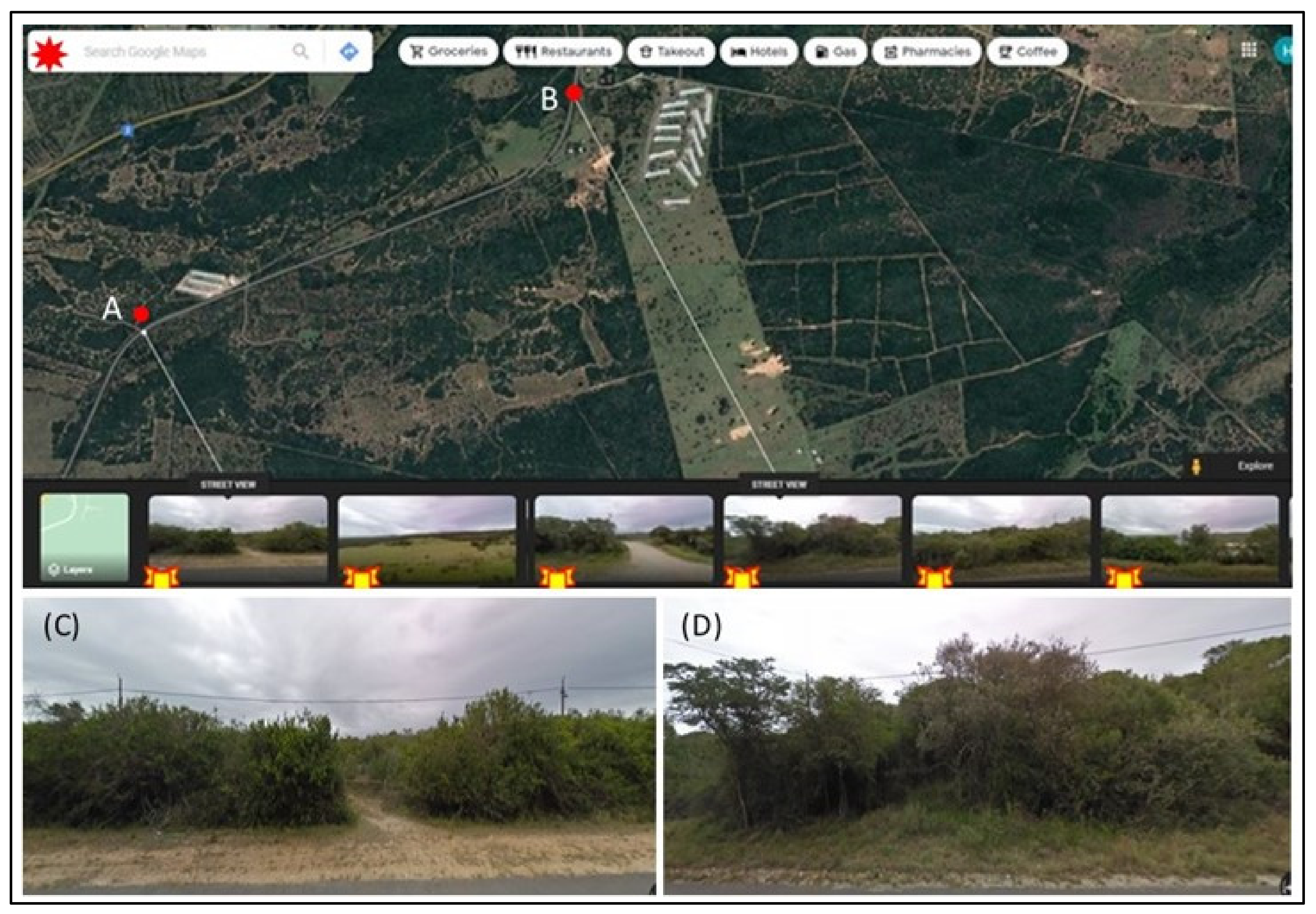
Supervised classification was conducted by segregating the images into two groups consisting of the most recent image of 2017 and the historical images of 1991, 2000 and 2009. This was followed by using 2/3 of the ground truth from field investigation to extract signatures for each of the five cover types following procedures suggested by Chen and Stow [65]. The extraction of signatures was further boosted by using Google Earth images [66] and the aerial photographs as collateral sources of ground truth. The former were used to aid the discrimination of different cover types based on geolocated roadside photographs that allowed additional signatures to be extracted (Figure 3).
The aerial photographs were used as ancillary sources of ground truth by displaying them and their corresponding SPOT images in geographically linked viewers and using the Linked Cursor tool to co-locate different cover types. Their correspondence was established by pairing them in the same order they are listed in Table 1. The extraction of signatures for dynamic cover types, such as surface water, crops and natural vegetation, was enhanced by using contextual detectors [67,68] and evidential reasoning [69]. No crops and excess water-intolerant vegetation types were expected in the estuary, for example.
This reasoning enhanced confident discrimination of other features based on location, tone and shape. Misclassification of vegetation and crops was addressed by digitizing all fields and overlaying the digitized layers on the initial map outputs. All classifications were based on the Maximum-likelihood classifier because, apart from performing better than the Minimum and Mahalanobis distance classifiers, it produces spectrally separable signatures and meaningful results [70,71]. Classification accuracies were determined by compiling confusion matrices following procedures suggested by Campbell [72]. Table 3 illustrates how these calculations were performed.
The figures in Table 3a are numbers of training samples that were extracted from the image during supervised classification with training site consisting of 4 pixels whose signatures were extracted by using a 2 × 2-pixel window. The shaded diagonal entries in Table 3a are training samples that were correctly classified during supervised classification. The other entries in each row are the training samples that were wrongly classified during signature-based image classification. For bare area, for example, out of the 14 samples that were extracted through interactive onscreen extraction of signatures, one sample was misclassified as cultivated land and another sample was also misclassified as noncultivated land. Accuracy levels for the remaining 1991, 2009 and 2017 map outputs were 83.93%, K = 0.757, 87.43%, K = 0.812, and 87.70%, K = 0.816, respectively. These accuracies were lower than the minimum 85% recommended by Anderson [73]. However, some authors [74,75] argue that many researchers have been misapplying this recommendation as a limit by ignoring that it was only suggested as a target for mapping a small number (~9) of broad land cover classes from 80 m resolution Landsat images.
Congalton and Green [76] go further to note that setting acceptable limits is misleading because classification accuracy is meant ‘to enable users to determine a map’s suitability for their specific needs and not to provide a basis for quality assessment’. The Kappa statistic used by many researchers for classification accuracy assessment has also been widely criticised as misleading and of little use for practical applications and decision making [77,78,79,80]. In view of these considerations, it is justifiable to conclude that the levels of accuracy that were achieved in this investigation are within acceptable limits.
3. Results and Statistical Analysis
Results
Results of this investigation are presented in the form of tables (Table 4 and Table 5). Table 4 shows percentage compositions and percentage changes in the spatial distributions of land cover types that were mapped. Table 5 shows the trend coefficients of these cover types and correlations between long-term changes in the five land cover types that were mapped and adjusted annual rainfall (AAR).
Simple linear trend analysis revealed (1) statistically insignificant negative trends for bare area, surface water, noncultivated land, adjusted annual rainfall (AAR) and long-term rainfall and (2) statistically insignificant positive trends for vegetation and cultivated land. MK trend analysis detected similar trends except for surface water. All correlations were weak (R2 < 0.64) and statistically insignificant except for the correlation between rainfall and surface water distribution (R2 = 0.813709).
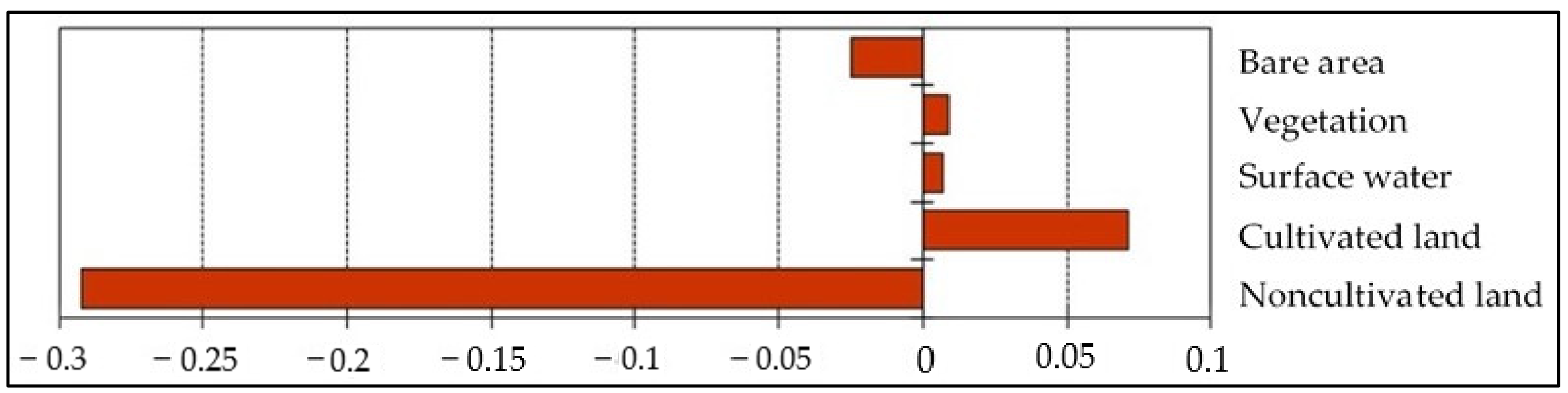
Long-term changes in all cover types were marginal (<8%), with vegetation and noncultivated land initially decreasing by 7.23% and 16.81%, respectively, between 1991 and 2000. Bare area, surface water and cultivated land increased by 8.92%, 5.54% and 9.58%, respectively. Overall, all changes were marginal (<8%) except for bare area, which decreased by 12.22%, and noncultivated land, which increased by 11.79% (Table 4). Statistical analysis was performed to ascertain the direction of change in rainfall and different cover types and the relationship between these variables. Table 5 shows (1) linear trend coefficients for the five cover types that were mapped and their SSE estimates and their p values, (2) linear trend coefficients for long-term annual rainfall (1991–2017) and the adjusted annual rainfall figures (AAR) for the four time slices (1991, 2000, 2009 and 2017) that were sampled for this investigation and (3) correlation coefficients for AAR and percentage changes in the five cover types that were mapped and Sen Slope Estimates for all cover types and rainfall.
Linear trend coefficients were computed in Excel and their accuracies cross-checked by performing the Mann–Kendall (M–K) trend test [81] and their magnitudes and the direction of change were determined by using Excel’s XLSTART plugin extension to calculate Sen Slope Estimates (SSE) [82]. A positive (negative) SSE indicates an upward (downward) trend [83]. The advantages of this test are provided elsewhere [84]. The strength of the association between rainfall and different cover types was determined by calculating the Pearson product-moment correlation coefficients and the statistical significance of each correlation (p) was determined by reference to the table of critical values at σ = 0.05.
Changes in all cover types were statistically insignificant but long-term rainfall exhibited a significant decrease.
4. Discussion
The results of this investigation point to marginal long-term changes (<8%) in all cover types, with vegetation and cultivated land decreasing. Interestingly, however, simple linear and MK trend analyses revealed discordant trends for surface water distribution (Table 5). The former detected a long-term decrease (y = −0.4261x + 9.657), while the latter detected a long-term increase (SSE = 0.007). Equally interesting is the fact the marginal increase in surface water distribution is not only consistent with what is expected in open estuarine ecosystems [85] but also in agreement with the established cryptic effects of SLR average increases of 1.6 and 1.8 mm yr−1 during the 20th century [86,87]. The major insight from these observations is that although SLR is indeed occurring, simplistic analysis can give a misleading sense of stability by failing to detect the hydrological response of estuaries to the gradual increase in SLR.
This assertion is supported by Bornman and co-authors [24], who report a potential SLR-induced loss of 30.24 ha in the neighbouring Swartkops River Estuary. In the GRE, the observed increase surface water, although marginal, is a phenomenon that can only be explained by SLR because it is an open estuary. This trend is a long-term liability which is the associated inundation of aesthetically valuable beach areas that are vital for tourism and the inland progression of seawater into terrestrial freshwater systems. The observed 0.44% increase in surface water for example (Table 4) translates into the submergence of ~7.64 ha of dryland over the period of the 26 years that were covered by this study. This cryptic phenomenon is now widely considered to be a climate change impact of extreme significance [88].
Although the small size of our sample (four time slices) might have skewed the trend by failing to capture subtle changes, it was able detect a decreasing trend in rainfall (Figure 4) that was confirmed by the robust MK analysis (Table 5). In addition, the only way surface water could have increased as rainfall declined (Figure 2a) is by replenishment from external supplies of which seawater is the only source. This reasoning is supported by the long-term decrease in the estuary’s freshwater supplies due to frequent occurrence of below-average rainfall (Figure 2b).
The periodic changes in vegetation suggest the combined influence of both human and climatic factors. Although human influence is confirmed by the documented explosive increase in citrus area and irrigated pastures after 2000 [51], this increase alone does not provide a convincing explanation of the observed increase in vegetation because cultivated land and vegetation were mapped separately. In the absence of cultivation, the most likely natural drivers of vegetation’s expansion include the frequent occurrence of below-average rainfall (Figure 2b) and significant long-term decrease in rainfall (Table 5). Although our mapping did not discriminate vegetation by species type, evidence indicates increasing infestation of the estuary’s fringes by woody invasives [56]. This trend is consistent with the well-established positive influence of frequent rainfall failures and climate-change-driven CO2 fertilization on the expansion of species that are adapted to soil moisture deficit conditions [89,90,91].
In water-stressed environments, rainfall failures create windows of opportunity for the expansion of species that are adapted to water-stressed conditions [92]. Given the immense variability of rainfall in this area, it is logical to associate the infestation of GRE by invasives with the long-term decrease in this area’s rainfall. This association has been observed in many parts of southern Africa where the expansion of vegetation species that are adapted to moisture deficit conditions is becoming increasingly recognised as one of the outcomes of deteriorating rainfall conditions [93,94]. This observation is interesting because it suggests that the substantial decrease in rainfall is one of the major drivers of the observed increase in vegetation and the reported expansion of invasives. The long-term implication of this phenomenon is the loss of biodiversity. Poor management of irrigated land also emerges as one the possible drivers.
There are 250 farmers in this area, 17 of whom are resource-poor farmers who do not have adequate resources to fully utilise the land at their disposal. The result is underutilised land which contributed to the increase in bare area because most RPFs cleared land for agriculture which they were not able to fully utilise [88]. This underutilisation was aggravated by successive of years of below-average rainfall after 2000 (Figure 2b). Over time, these semi-abandoned landholdings became hospitable areas for the expansion of encroachers, hence the observed decrease in bare area as vegetation and surface water increased (Table 4).
The marginal increase in surface water can be explained by SLR and not rainfall, which significantly decreased (p = 0.0411, 0.05) between 1991 and 2017 (Table 5). Evidence from the literature shows that the global average sea level rose at a rate of ~1.8 mm year−1 between 1961 and 2003 and at higher rate of ~3.1 mm year−1 between 1993 and 2003 [88]. These trends are supported by (1) the failure of the Knysna Estuary in Western Cape Province to keep pace with RSL rise and the potential loss of 40% of its intertidal salt marsh to drowning by 2100 [23], (2) similar trends in the Swartkops River Estuary in the Eastern Cape province [24], (3) sea-level-driven marsh expansion in other areas worldwide [27,95] and (4) the international recognition of land ice melting and the global thermal expansion of the oceans as major threats to estuaries [96]. The potential cumulative long-term impacts of this marginal increase include but are not limited to (1) the irreversible loss of cultivable land in the estuary’s flood plain areas, (2) the drowning of recreational space in sand beaches and habitable land for human settlement, (3) the contamination of terrestrial freshwater reserves from the landward migration of seawater and (4) the alteration of the existing zonation and composition of both dryland and wetland vegetation communities in favour of saline soil and saltwater-tolerant species.
As reported by many researchers [97,98,99,100], small changes similar to the marginal surface water increase we observed must not be trivialised because they often signal the landward migration of the saltwater fringe into coastal freshwater systems. The decrease in bare area (Figure 4) does not imply improvement. This decrease can be explained by SL-driven landward migration of seawater. The same decrease is also indicative of the documented agriculture-driven conversion of natural ecosystems [18,99]. The decrease in rainfall also emerges as one of the factors driving these changes.
This assertion is supported by the periodic variation of cultivated land in tandem with changes in rainfall. In 2000, for example, the amount of land under cultivation drastically increased as rainfall increased, with the reverse occurring after 2009 when rainfall declined (Figure 2a). This correspondence suggests that irrigation alone does not explain the trend in cultivated land. The influence of rainfall appears to be determined not only by absolute amount, per se, but also by its concentration in autumn and spring. This skewed distribution implies water deficits in summer and winter which compel farmers to downscale operations. This situation translates into more cultivation in good rainfall (Table 4), but excessive rainfall can also reduce cultivation by flooding land, as happened in 1971 when 24% of irrigated land was buried by sediments to depths of 3 m [46]. These scenarios are indicative of how climate extremes and human interference often reinforce each other to trigger adverse changes that are not easily reversible.
Although irrigation is this area’s mainstay of agriculture, there is a fixed 800 m3/ha that cannot be exceeded in periods of rainfall failures and drought [17]. This rationing is supported by the reduced allocation of water to 35% of each farmer’s requirements during the 2005–2006 drought [51,52] and the more recent reduction in allocations to 20% of each farmer’s requirements in 2021 [100,101]. This scenario requires efficient utilisation of limited water supplies in order to minimise the risk of passing irreversible thresholds. Unfortunately, not all farmers in this area are able to do so, as demonstrated by the changes in cultivated land (Table 4) in tandem with the changes in rainfall (Figure 2a). What this suggests is that in this area, the influence of irrigation on the changes in cultivated area must be interpreted within the context of a technology whose functioning is dependent on the availability of water from upstream dams.
5. Conclusions
The objective of this paper was to ascertain the nature, causes, extent and direction of changes in land cover in the GRE. This was accomplished by (1) quantifying changes in land cover and identifying the major drivers of these changes and (2) determining the long-term direction of these changes over a period of 26 years between 1991 and 2017. Changes in all cover types were marginal, but the GRE appears to be threatened by both anthropogenic and climate stressors with human intervention through the conversion of land to cultivation, overgrazing in the catchment areas and the impoundment of surface water for irrigation emerging as the greatest. Mitigating the threats associated with these stressors requires (1) a better understanding of what controls estuarine habitats and the changes that they may undergo by quantifying and monitoring the dynamic effects of both human and natural factors and (2) the informed adoption of sustainable resource use practices (SRUP).
Selected examples of SRUP for the GRE and others elsewhere include (1) the adoption of water-saving irrigation techniques and crop varieties that mature in shorter time periods, (2) increasing crop water productivity by focusing on high-value and low-water-demanding varieties, (3) shortening crop growing seasons to save water by shifting to varieties that mature in shorter time periods, (4) encouraging the adoption of sound land management practices that do not promote the spread of alien invasive species, (5) empowering emerging farmers through training and the provision of structured financial support, (6) minimising the destructive effects of high-magnitude floods by improving flood control measures, (7) land use zoning to protect the estuary by prohibiting the extension of human activities into sensitive areas, (8) enforcing regulations that are designed to ensure responsible stewardship, (9) constant monitoring to enable timely implementation of appropriate interventions and (10) incentivising users of the estuary’s resources to voluntarily adopt appropriately informed management strategies by offering tangible benefits that confer a sense of ownership.
Although the GRE is considered to be in fair conservation condition [102], the results of this study indicate that it is under more considerable threats than commonly perceived. These threats should not be ignored but actively confronted and built upon. Research can contribute to this call by making concerted efforts to enhance our understanding of how the incremental effects of small changes may diminish the sustainability of estuarine ecosystems. Future research can contribute more to policy and ecosystem-based management by exploring innovative ways through which the cumulative impacts of individual stressors or groups of stressors can be timely isolated and addressed before it is too late.
Accomplishing this requires the regular monitoring of stressors that have potentials for spatial and temporal accumulation. This investigation contributed to this objective by pinpointing some of the underestimated and trivialised stressors that threaten the sustainability of the GRE. Admittedly, however, some the major limitations of this investigation’s findings include its limited time span, local focus, lack of suitable nonclimatic data and lack of reliable rainfall records for the period before 1990. These limitations impede analysis at broader temporal and spatial scales. These constraints point to gaps that need to be bridged by regularly monitoring key stressors that impact the environment and embracing new ways of investigative enquiry instead of conducting business as usual. We conclude by inviting researchers elsewhere to build on this initiative by formulating strategies that can be used to address the threats confronting estuarine ecosystems for the benefit of present and future generations.
Author Contributions
Conceptualization, M.A.N., K.R.G. and H.H.; methodology, M.A.N., K.R.G. and H.H.; validation, M.A.N., K.R.G. and H.H; fieldwork, M.A.N.; formal analysis, H.H., M.A.N. and K.R.G.; writing—review and editing, H.H., M.A.N. and K.R.G.; project administration, K.R.G.; funding acquisition, H.H. All authors have read and agreed to the published version of the manuscript.
Funding
This research received was funded by South African Institute for Aquatic Biodiversity (SAIAB).
Institutional Review Board Statement
Not Applicable.
Informed Consent Statement
Not Applicable.
Data Availability Statement
The SPOT satellite images used in this study were obtained from the South African Space Agency (SANSA) through the SANSA Earth Observation Online Catalogue (http://catalogue.sansa.org.za/). Aerial photographs were obtained over the counter from the National Geo-Spatial Information (NGI) sales (https://ngi.dalrrd.gov.za/index.php/contact-ngi). Rainfall data was also acquired over the counter from the South African Weather Services (SAWS) (https://www.weathersa.co.za/home/equiries).
Acknowledgments
The authors thank South African National Space Agency (SANSA) for satellite imagery, South African Weather Service (SAWS) for rainfall data and National Geo-spatial Information (NGI) for aerial photography. We also thank John Richardson for editorial assistance and the anonymous reviewers whose comments helped us to improve this paper.
Conflicts of Interest
The authors declare no conflict of interest.
References
- Whitfield, A.K.; Elliott, M. Ecosystem and biotic classifications of estuaries and coasts. In Treatise on Estuaries and Coasts; Wolanski, E., McLusky, D.S., Eds.; Elsevier: Amsterdam, The Netherlands, 2011; pp. 99–124. Available online: https://www.sciencedirect.com/science/article/pii/B978012374711200108X (accessed on 17 June 2021). [CrossRef]
- James, N.C.; Harrison, T.D. A preliminary survey of the estuaries on the southeast coast of South Africa, Cape St Francis–Cape Padrone, with particular reference to the fish fauna. Trans. R. Soc. S. Afr. 2010, 65, 69–84. [Google Scholar] [CrossRef]
- Woodwell, G.M.; Rich, P.H.; Hall, C.A.S. Carbon in estuaries. In Carbon and the Biosphere; Woodwell, G.M., Peron, E.V., Eds.; National Technical Information Service: Springfield, VA, USA, 1973; pp. 221–240. [Google Scholar]
- Barbier, E.B.; Hacker, S.D.; Kennedy, C.; Koch, E.W.; Stier, A.C.; Silliman, B.R. The value of estuarine and coastal ecosystem services. Ecol. Monogr. 2011, 81, 169–193. [Google Scholar] [CrossRef]
- Shepard, C.C.; Crain, C.M.; Beck, M.W. The protective role of coastal marshes: A systematic review and meta-analysis. PLoS ONE 2011, 6, e27374. [Google Scholar] [CrossRef] [PubMed]
- De Groot, R.S.; Wilson, M.A.; Boumans, R.M.J. A typology for the classification, description and valuation of ecosystem functions, goods and services. Ecol. Econ. 2002, 41, 393–408. [Google Scholar] [CrossRef] [Green Version]
- Boyd, A.J.; Barwell, L.; Taljaard, S. Report on the National Estuaries Workshop: 3–5 May 2000 Port Elizabeth, South Africa. Issue 2 of Marine and Coastal Management Implementation Workshops. Department of Environmental Affairs and Tourism. Marine and Coastal Management. MCM, DEA & T and CSIR Environmentek. 2000. Available online: https://books.google.co.za/books?id=2_-XXwAACAAJ&dq=inauthor:%22South+Africa.+Department+of+Environmental+Affairs+and+Tourism.+Marine+and+Coastal+Management%22&hl=en&sa=X&redir_esc=y (accessed on 17 February 2021).
- Van Niekerk, L.; Taljaard, S.; Adam, J.B.; Lambert, D.J.; Huizinga, P.; Turpie, J.K.; Wooldridge, T.H. An environmental flow determination method for integrating multiple-scale ecohydrological and complex ecosystem processes in estuaries. Sci. Total Environ. 2019, 656, 482–494. [Google Scholar] [CrossRef]
- Lotze, H.K.; Lenihan, H.S.; Bourque, B.J.; Bradbury, R.H.; Cooke, R.G.; Kay, M.C.; Kidwell, S.M.; Kirby, M.X.; Peterson, C.H.; Jackson, J.B.C. Depletion, degradation, and recovery potential of estuaries and coastal seas. Science 2006, 312, 1806–1809. [Google Scholar] [CrossRef]
- Driver, A.; Maze, K.; Lombard, A.T.; Nel, J.; Rouget, M.; Turpie, J.K.; Cowling, R.M.; Desmet, P.; Goodman, P.; Harris, J.; et al. South African National Spatial Biodiversity Assessment 2004: Summary Report; South African National Biodiversity Institute (SANBI Publishing): Pretoria, South Africa, 2004. [Google Scholar]
- Snow, G.C.; Adams, J.B.; Bate, G.C. Effect of river flow on estuarine microalgal biomass and distribution. Estuar. Coast. Shelf Sci. 2000, 51, 255–266. [Google Scholar] [CrossRef]
- Lemley, D.A.; Adams, J.B.; Strydom, N.A. Triggers of phytoplankton bloom dynamics in permanently eutrophic waters of a South African estuary. Afr. J. Aquat. Sci. 2018, 43, 229–240. [Google Scholar] [CrossRef]
- Lemley, D.A.; Adams, J.B.; Taljaard, S. Comparative assessment of two agriculturally influenced estuaries: Similar pressure, different response. Mar. Pollut. Bull. 2017, 117, 136–147. [Google Scholar] [CrossRef]
- Lawrie, R.A.; Stretch, D.D.; Perissinotto, R. The effects of wastewater discharges on the functioning of a small temporarily open/closed estuary. Estuar. Coast. Shelf Sci. 2010, 87, 237–245. [Google Scholar] [CrossRef]
- Perissinotto, R.; Blair, A.; Connell, A.; Demetriades, N.T.; Forbes, A.T.; Harrison, T.H.; Lyer, K.; Joubert, M.; Kibirige, I.; Mundree, S.; et al. Contributions to Information Required for the Implementation of Resource Directed Measures for Estuaries (Volume 2). Responses of the Biological Communities to Flow Variation and Mouth State in Two KwaZuluNatal Temporarily Open/closed Estuaries; WRC Report No. 1247/2/04; Water Research Commission: Pretoria, South Africa, 2004. [Google Scholar]
- Schumann, E.; Pearce, M. Freshwater inflow and estuarine variability in the Gamtoos Estuary, South Africa. Estuaries 1997, 20, 124–133. [Google Scholar] [CrossRef]
- Heinecken, T.J.E.; Bickerton, I.B.; Heydorn, A.E.F. A Summary of Studies of the Pollution Input by Rivers and Estuaries Entering False Bay; CSIR Report T/SEA 8301; Council for Scientific and Industrial Research: Stellenbosch, South Africa, 1983. [Google Scholar]
- Schumann, E.H.; Pearce, M.W. The Effect of Land Use on Gamtoos Estuary Water Quality. Report to the Water Research Commission by the Department of Geology, University of Port Elizabeth. WRC Report No. 503/1/97. Nd. Available online: http://www.wrc.org.za/wp-content/uploads/mdocs/503-1-97.pdf (accessed on 21 May 2021).
- Pearce, M.W.; Schumann, E.H. The impact of irrigation return flow on aspects of the water quality of the upper Gamtoos Estuary, South Africa. Water SA 2001, 27, 367–372. [Google Scholar] [CrossRef] [Green Version]
- Adams, J.B.; Van Niekerk, L. Ten principles to determine environmental flow requirements for temporarily closed estuaries. Water 2020, 12, 1944. [Google Scholar] [CrossRef]
- Human, L.R.D.; Adams, J.B. Reeds as indicators of nutrient enrichment in a small temporarily open/closed South African estuary. Afr. J. Aquat. Sci. 2011, 36, 167–179. [Google Scholar] [CrossRef]
- Morant, P.; Quinn, N. Influence of man and management of South African estuaries. In Estuaries of South Africa; Allanson, B.R., Baird, D., Eds.; Cambridge University Press: Cambridge, UK, 1999; pp. 289–321. [Google Scholar]
- Raw, J.L.; Riddin, T.; Wasserman, J.; Lehman, T.W.K.; Bornman, T.G.; Adams, J.B. Salt marsh elevation and responses to future sea-level rise in the Knysna Estuary, South Africa. Afr. J. Aquat. Sci. 2020, 45, 49–64. [Google Scholar] [CrossRef]
- Bornman, T.G.; Schmidt, J.; Adams, J.B.; Mfikili, A.N.; Farre, R.E.; Smit, A.J. Relative sealevel rise and the potential for subsidence of the Swartkops Estuary intertidal salt marshes, South Africa. S. Afr. J. Bot. 2016, 107, 91–100. [Google Scholar] [CrossRef]
- Cahoon, D.R.; Lynch, J.C.; Roman, C.T.; Schmit, J.P.; Skidds, D.E. Evaluating the relationship among wetland vertical de-velopment, elevation capital, sea-level rise, and tidal marsh sustainability. Estuaries Coasts 2019, 42, 1–15. [Google Scholar] [CrossRef]
- Enwright, N.M.; Griffith, K.T.; Osland, M.J. Barriers to and opportunities for landward migration of coastal wetlands with sea-level rise. Front. Ecol. Environ. 2016, 14, 307–316. [Google Scholar] [CrossRef]
- Kirwan, M.L.; Walters, D.C.; Reay, W.G.; Carr, J.A. Sea level driven marsh expansion in a coupled model of marsh erosion and migration. Geophys. Res. Lett. 2016, 43, 4366–4373. [Google Scholar] [CrossRef] [Green Version]
- Whitfield, A.; Bate, G. A Review of Information on Temporarily Open/Closed Estuaries in the Warm and Cool Temperate Biogeographic Regions of South Africa, with Emphasis on the Influence of River Flow on These Systems; WRC Report No. 1581/1/07; Water Research Commission: Pretoria, South Africa, 2007. [Google Scholar]
- Taljaard, S.; van Niekerk, L.C.A.P.E. Estuaries Programme. Proposed Generic Framework for Estuary Management Plans. Version 1.1; CSIR Report No. CSIR/NRE/CO/ER/2009/0128/A; Council for Scientific and Industrial Research: Stellenbosch, South Africa, 2009. [Google Scholar]
- Thomas, C.M.; Perissinotto, R.; Kibirige, I. Phytoplankton biomass and size structure in two South African eutrophic, temporarily open/closed estuaries. Estuar. Coast. Shelf Sci. 2005, 65, 223–238. [Google Scholar] [CrossRef]
- UNEP/Nairobi Convention Secretariat. Transboundary Diagnostic Analysis of Land-based Sources and Activities Affecting the Western Indian Ocean Coastal and Marine Environment; UNEP Nairobi: Nairobi, Kenya, 2009; Available online: https://nairobiconvention.org/CHM%20Documents/WIOSAP/-Transboundary%20Diagnostic%20Analysis%20of%20Land-based%20Sources%20and%20Activities%20in%20the%20Western%20Indian%20Ocean%20Region.-2009Transboundary%20Diagnostic%20Analysis%20of%20Land-based%20Sources%20and%20Activities-1.pdf (accessed on 17 June 2021).
- James, N.C.; van Niekerk, L.; Whitfield, A.K.; Potts, W.M.; Götz, A.; Paterson, A.W. Effects of climate change on South African estuaries and associated fish species. Clim. Res. 2013, 7, 233–248. [Google Scholar] [CrossRef] [Green Version]
- James, N.C.; Whitfield, A.K.; Cowley, P.D. Preliminary indications of climate-induced change in a warm-temperate South African estuarine fish community. Fish Biol. 2008, 72, 1855–1863. [Google Scholar] [CrossRef]
- Meynecke, J.O.; Yip Lee, S.; Duke, N.C.; Warnken, J. Effect of rainfall as a component of climate change on estuarine fish production in Queensland, Australia. Estuar. Coast. Shelf Sci. 2006, 69, 491–504. [Google Scholar] [CrossRef]
- Clark, B.M. Climate change: A looming challenge for fisheries management in southern Africa. Mar. Policy 2006, 2006. 30, 84–95. [Google Scholar] [CrossRef]
- Odum, W. Environmental degradation and the tyranny of small decisions. BioScience 1982, 32, 728–729. [Google Scholar] [CrossRef]
- Dale, V.H. The relationship between land-use change and climate change. Ecol. Appl. 1997, 7, 753–769. [Google Scholar] [CrossRef]
- Lambin, E.F.; Turner, B.L.; Geist, H.E.; Agbola, S.B.; Angelsen, A.; Bruce, J.W.; Coomes, O.T.; Dirzo, R.; Fischer, G.; George, P.S.; et al. The causes of land-use and land-cover change: Moving beyond the myths. Glob. Environ. Chang. 2001, 11, 261–269. [Google Scholar] [CrossRef]
- Adams, J.B.; Taljaard, S.; van Niekerk, L.; Lemley, D.A. Nutrient enrichment as a threat to the ecological resilience and health of South African microtidal estuaries. Afr. J. Aquat. Sci. 2020, 45, 23–40. [Google Scholar] [CrossRef] [Green Version]
- Jezewski, W.A.; Roberts, C.P.R. Estuarine and Lake Freshwater Requirements. Department of Water Affairs; Technical Report No. TR 129; DWAF: Pretoria, South Africa, 1986; p. 36. [Google Scholar]
- Whitfield, A.K.; Bate, G.C.; Adams, J.B.; Cowle, P.D.; Froneman, P.W.; Gama, P.T.; Strydom, N.A.; Taljaard, S.; Theron, A.K.; Turpie, J.K.; et al. A review of the ecology and management of temporarily open/closed estuaries in South Africa, with particular emphasis on river flow and mouth state as primary drivers of these systems. Afr. J. Mar. Sci. 2012, 34, 163–180. [Google Scholar] [CrossRef]
- Thomas Kwadwo Gyedu-Ababio, K.T. Pollution status of two river estuaries in the Eastern Cape, South Africa, based on Benthic Meiofauna analyses. J. Water Resour. Prot. 2011, 3, 464–486. [Google Scholar] [CrossRef] [Green Version]
- Marais, J.F.K. Fish abundance and distribution in the Gamtoos estuary with notes on the effect of floods. S. Afr. J. Zool. 1983, 18, 103–109. [Google Scholar] [CrossRef] [Green Version]
- Dupra, V.; Smith, S.V.; Marshall Crossland, J.I.; Crossland, C.J. Land-Ocean Interactions in the Coastal Zone (LOICZ). Estuarine Systems of Sub-Saharan Africa: Carbon, Nitrogen and Phosphorus Fluxes. LOICZ Reports & Studies 18. 2001. Available online: https://s3-eu-west-2.amazonaws.com/futureearthcoasts/wp-content/uploads/2018/05/30150945/LOICZ-RS18.pdf (accessed on 11 April 2022).
- Heydorn, A.E.F.; Grindley, J.R. Estuaries of the Cape, Part II. Synopses of Available Information on Individual Systems; Report No.7: Gamtoos. CSIR Res. Rep. 406; National Research Institute for Oceanology Council for Scientific and Industrial Research: Stellenbosch, South Africa, 1981; pp. 1–40. [Google Scholar]
- Shone, R.W.; Nolte, C.C.; Booth, P.W.K. Pre-Cape rocks of the Gamtoos area—A complex tectonostratigraphic package preserved as a horst block. S. Afr. J. Geol. 1990, 93, 616–621. [Google Scholar]
- Alexander, W.J.R. August 1971 Gamtoos Valley Floods. 1971. Available online: https://www.baviaans.net/articles/august-1971-gamtoos-valley-floods-03-2019-d1 (accessed on 19 February 2021).
- Gamtoos History & Geology. Available online: https://www.baviaans.net/page/geology_and_history (accessed on 13 April 2022).
- Rogers, G. Gamtoos Estuary Closed for the First Time in 70 Years. 2018. Available online: https://www.heraldlive.co.za/news/2018-07-11-gamtoos-estuary-closed-for-first-time-in-70-years/ (accessed on 16 May 2021).
- Kopke, D. The climate of the Eastern Cape. In Towards an Environmental Plan for the Eastern Cape; Bruton, M.N., Gess, F.W., Eds.; Rhodes University: Grahamstown, South Africa, 1988; pp. 44–52. [Google Scholar]
- Van der Burg, L. Valuing the Benefits of Restoring the Water Regulation Services, in the Subtropical Thicket Biome: A Case Study in the ‘Baviaanskloof Gamtoos watershed’, South-Africa. Master’s Thesis, Wageningen University, Wageningen, The Netherlands, 2008. Available online: http://media.dirisa.org/inventory/archive/presence-learning-network/documents/van-der-burg-lennart_2008_benefits-restoring-water-regulation-gamtoos.pdf (accessed on 26 May 2021).
- Scharler, U.M.; Baird, D. The nutrient status of the agriculturally impacted Gamtoos Estuary, South Africa, with special reference to the river-estuarine interface region (REI). Aquat. Conserv. Mar. Freshw. Ecosyst. 2003, 13, 99–119. [Google Scholar] [CrossRef]
- DEA (Department of Environmental Affairs). Climate Change Adaptation Plans for South African Biomes; Kharika, J.R.M., Mkhize, N.C.S., Munyai, T., Khavhagali, V.P., Davis, C., Dziba, D., Scholes, R., van Garderen, E., von Maltitz, G., Le Maitre, D., et al., Eds.; South African National Biodiversity Institute: Pretoria, South Africa, 2015. Available online: https://www.gov.za/documents/climate-change-adaptation-plans-south-african-biomes-18-jul-2016-0000 (accessed on 16 August 2021).
- Mucina, L.; Rutherford, M.C. (Eds.) The Vegetation of South Africa, Lesotho and Swaziland. Strelitzia 19; South African National Biodiversity Institute: Pretoria, South Africa, 2006. [Google Scholar]
- Enviro-Fish Africa. Gamtoos Estuarine Management Plan Vol. II. 2008. Available online: http://fred.csir.co.za/project/CAPE_Estuaries/documents/Gamtoos%20Draft%20EMP.pdf (accessed on 27 May 2021).
- Garcia-Rodriguez, F.D.G. The Determination and Distribution of Microbenthic Chlorophyll—A in Selected South Cape Estuaries. Master’s Thesis, University of Port Elizabeth, Port Elizabeth, South Africa, 1993. [Google Scholar]
- Scharler, U.M.; Baird, D. The filtering capacity of selected Eastern Cape estuaries, South Africa. Water SA 2006, 31, 483–490. [Google Scholar] [CrossRef] [Green Version]
- Consortium for Estuarine Research and Management (CERM). Studies on the River-Estuary Interface Region of Selected Eastern Cape Estuaries. Report No: 756/1/03. 2003. Available online: http://www.fwr.org/wrcsa/756103.htm (accessed on 17 April 2019).
- Watling, R.J.; Watling, H.R. Metal Surveys in South African Estuaries vs. Kromme and Gamtoos Rivers (St Francis Bay). Water SA 1982, 8, 187–191. [Google Scholar]
- ATCOR-2/3. Atmospheric/Topographic Correction of Satellite Imagery, ERDAS Imagine ATCOR-2/3 User Guide, Version 9.0.2. 2016. Available online: https://www.rese.ch/pdf/atcor3_manual.pdf (accessed on 21 February 2019).
- South Africa National Space Agency (SANSA). Available online: https://www.sansa.org.za/ (accessed on 17 June 2020).
- NGI National Geo-Spatial Information (NGI). Available online: http://www.ngi.gov.za/index.php/contact-ngi (accessed on 16 March 2018).
- Di Gregorio, A. Land Cover Classification System: Classification Concepts and User Manual: LCCS (No. 8); FAO: Rome, Italy, 2005; Available online: http://www.fao.org/3/a-i5232e.pdf (accessed on 21 February 2019).
- Thomlinson, J.R.; Bolsta, P.V.; Cohen, W.B. Coordinating methodologies for scaling landcover classifications from site-specific to global: Steps toward validating global map products. Remote Sens. Environ. 1999, 70, 16–28. [Google Scholar] [CrossRef]
- Chen, D.; Stow, D.A.V. The effect of training strategies on supervised classification at different spatial resolutions. Photogramm. Eng. Remote Sens. 2002, 68, 1155–1161. [Google Scholar]
- Available online: https://www.google.com/maps/@-33.9321432,25.1012905,2194m/data=!3m1!1e3?hl=en-US (accessed on 15 June 2017).
- Peddle, D.R.; Ferguson, D.T. Optimization of multisource data analysis: An example using evidential reasoning for GIS data classification. Comput. Geosci. 2002, 28, 45–52. [Google Scholar] [CrossRef]
- Franklin, S.E.; Wulder, M.A. Remote sensing methods in medium spatial resolution satellite data land cover classification of large areas. Prog. Phys. Geogr. 2002, 26, 173–205. [Google Scholar] [CrossRef]
- Ayele, G.T.; Tebeje, A.K.; Demissie, S.S.; Belete, M.A.; Jemberrie, M.A.; Teshome, W.M.; Mengistu, D.T.; Teshale, E. Time series land cover mapping and change detection analysis using Geographic Information System and Remote Sensing, Northern Ethiopia. Air Soil Water Res. 2018, 11, 1–18. [Google Scholar] [CrossRef] [Green Version]
- Abd, H.A.A.; Alnajjar, H.A. Maximum likelihood for land-use/land-cover mapping and change detection using Landsat satellite images: A case study “South of Johor”. Int. J. Comput. Eng. Res. 2013, 3, 26–33. [Google Scholar]
- Lu, D.; Weng, Q. A survey of image classification methods and techniques for improving classification performance. Int. J. Remote Sens. 2007, 28, 823–870. [Google Scholar] [CrossRef]
- Campbell, J.B. Introduction to Remote Sensing, 3rd ed.; Taylor and Francis: New York, NY, USA, 2002. [Google Scholar]
- Anderson, J.R.; Hardy, E.E.; Roach, J.T.; Witmer, R.E. A Land Use and Land Cover Classification System for Use with Remote Sensor Data. Geological Survey Professional Paper 671. 1976. Available online: https://pubs.usgs.gov/pp/0964/report.pdf (accessed on 14 July 2021).
- Foody, G.M. Harshness in image classification accuracy assessment. Int. J. Remote Sens. 2008, 29, 3137–3158. [Google Scholar] [CrossRef] [Green Version]
- Trodd, N.M. Uncertainly in land cover mapping for modelling land cover change. Int. J. Remote Sens. 1995, 25, 1235–1252. [Google Scholar]
- Congalton, R.G.; Green, K. A practical look at the sources of confusion in error matrix generation. Photogrametric Eng. Remote Sens. 1993, 59, 641–654. [Google Scholar]
- Pontius, R.G., Jr.; Thontteh, O.; Chen, H. Components of information for multiple resolution comparison between maps that share a real variable. Environ. Ecol. Stat. 2008, 15, 111–142. [Google Scholar] [CrossRef]
- Stehman, S.V.; Czaplewski, R.L. Design and analysis for thematic map accuracy assessment: Fundamental principles. Remote Sens. Environ. 1998, 64, 331–344. [Google Scholar] [CrossRef]
- Pontius, R.G.; Millones, M. Death to Kappa: Birth of quantity disagreement and allocation disagreement for accuracy assessment. Int. J. Remote Sens. 2011, 32, 4407–4429. [Google Scholar] [CrossRef]
- Gilbert, R.O. Statistical Methods for Environmental Pollution Monitoring; Van Nostrand Reinhold Co.: New York, NY, USA, 1987. Available online: https://www.osti.gov/servlets/purl/7037501/;Statistical (accessed on 24 June 2021).
- Sen, P.K. Estimates of the regression coefficient based on Kendall’s tau. J. Am. Stat. Assoc. 1968, 63, 1379–1389. [Google Scholar] [CrossRef]
- Gocic, M.; Trajkovic, S. Analysis of changes in meteorological variables using Mann-Kendall and Sen’s slope estimator statistical tests in Serbia. Glob. Planet. Chang. 2013, 100, 172–182. [Google Scholar] [CrossRef]
- Pandit, D.V. Seasonal rainfall trend analysis. Int. J. Eng. Res. Appl. 2016, 6, 69–73. [Google Scholar]
- Hamandawana, H.; Atyosi, Y.; Bornman, T.G. Multi-temporal reconstruction of long-term changes in land cover in and around the Swartkops River Estuary, Eastern Cape Province, South Africa. Environ. Monit. Assess. 2020, 192, 173. [Google Scholar] [CrossRef] [PubMed]
- Prandle, D. Vulnerability of Estuaries to Sealevel Rise Stage 1: A Review. 2010. Available online: https://assets.publishing.service.gov.uk/government/uploads/system/uploads/attachment_data/file/291214/scho0310bsac-e-e.pdf (accessed on 17 January 2022).
- Church, J.A.; White, N.J. Sea-level rise from the late 19th to early 21st century. Surv. Geophys. 2011, 32, 585–602. [Google Scholar] [CrossRef] [Green Version]
- Jevrejeva, S.; Moore, J.C.; Grinsted, A.; Woodworth, P.L. Recent global sea level acceleration started over 200 years ago? Geophys. Res. Lett. 2008, 35, L08715. [Google Scholar] [CrossRef]
- CES (Coastal & Environmental Services). Eastern Cape Climate Change Response Strategy. 2011. Available online: https://www.cityenergy.org.za/uploads/resource_182.pdf (accessed on 31 May 2021).
- Polley, H.W.; Johnson, H.B.; Mayeux, H.S. Carbon dioxide and water fluxes of C3 annuals and C3 and C4 perennials at subambient CO2 concentrations. Funct. Ecol. 1992, 6, 693–703. [Google Scholar] [CrossRef]
- Midgely, G.F.; Bond, W.J.; Roberts, R.; Wand, S.J.E. Potential Cause of Changes in Savanna Tree Success Due to Rising Atmospheric CO2. Towards Sustainable Management in the Kalahari Region–Some Essential Background Issues; Ringrose, S., Chanda, R., Eds.; University of Botswana: Gaborone, Botswana, 2000; pp. 166–170. [Google Scholar]
- Scheiter, S.; Higgins, S.I. Impacts of climate change on the vegetation of Africa: An adaptive dynamic vegetation modelling approach. Glob. Chang. Biol. 2009, 15, 2224–2246. [Google Scholar] [CrossRef]
- Hamandawana, H.; Chanda, R.; Eckardt, F. Natural and human-induced environmental changes in the distal reaches of Botswana’s Okavango Delta. J. Land Use Sci. 2007, 2, 57–78. [Google Scholar] [CrossRef]
- Masiza, W.; Hamandawana, H.; Chingombe, W. Monitoring changes in land use and land cover to ascertain the nature, causes and extent of degradation in the Savannas of Raymond Mhlaba Local Municipality, Eastern Cape, South Africa. Int. J. Environ. Stud. 2022, 79, 19–36. [Google Scholar] [CrossRef]
- Sankaran, M. Droughts and the ecological future of tropical savanna vegetation. J. Ecol. 2019, 107, 1531–1549. [Google Scholar] [CrossRef] [Green Version]
- Fagherazzi, S.; Anisfeld, S.C.; Blum, L.K.; Emily, V.; Long, E.V.; Feagin, R.A.; Fernandes, A.; Kearney, W.S.; Williams, K. Sea level rise and the dynamics of the marsh-upland boundary. Front. Environ. Sci. 2019, 7, 25. [Google Scholar] [CrossRef]
- Slangen, A.B.A.; Katsman, C.A.; Van de Wal, R.S.W.; Vermeersen, L.L.A.; Riva, R.E.M. Towards regional projections of twenty-first century sea-level change based on IPCC SRES scenarios. Clim. Dyn. 2012, 38, 1191–1209. [Google Scholar] [CrossRef] [Green Version]
- Idowu, T.E.; Lasisi, K.H. Seawater intrusion in the coastal aquifers of East and Horn of Africa: A review from a regional perspective. Sci. Afr. 2020, 8, e00402. [Google Scholar] [CrossRef]
- Chang, S.W.; Clement, P.; Simpson, M.J.; Lee, K.-K. Does sea-level rise have an impact on saltwater intrusion? Adv. Water Resour. 2011, 34, 1283–1291. [Google Scholar] [CrossRef] [Green Version]
- Werner, A.D.; Bakker, M.; Post, V.E.A.; Vandenbohede, A.; Lu, C.; Ataie, B.; Simmons, C.T.; Barry, D.A. Seawater intrusion processes, investigation, and management: Recent advances and future challenges. Adv. Water Resour. 2013, 51, 3–26. [Google Scholar] [CrossRef]
- Department of Forestry, Fisheries and Environment. The Garden Route Environmental Management Framework. 2010; pp. 1–168. Available online: https://www.dffe.gov.za/sites/default/files/docs/gardenroute_finalreport.pdf (accessed on 28 January 2022).
- Daniels, N. Gamtoos River Valley Drought Endangers Citrus Harvest. 2021. Available online: https://www.iol.co.za/capetimes/news/gamtoos-river-valley-drought-endangers-citrus-harvest-d9f4b156-4d2f-405f-a593-96acea8db61c (accessed on 17 January 2022).
- Turpie, J.K. Improving the Biodiversity Importance Rating of Estuaries. Water Research Commission Report, Water Research Commission, Pretoria, South Africa. 2004. Available online: http://www.wrc.org.za/wp-content/uploads/mdocs/WaterSA_2002_02_1386.pdf (accessed on 19 February 2022).
Figure 1.
Location of Gamtoos river estuary in Kouga Local Municipality, Eastern Cape province, South Africa.
Figure 1.
Location of Gamtoos river estuary in Kouga Local Municipality, Eastern Cape province, South Africa.
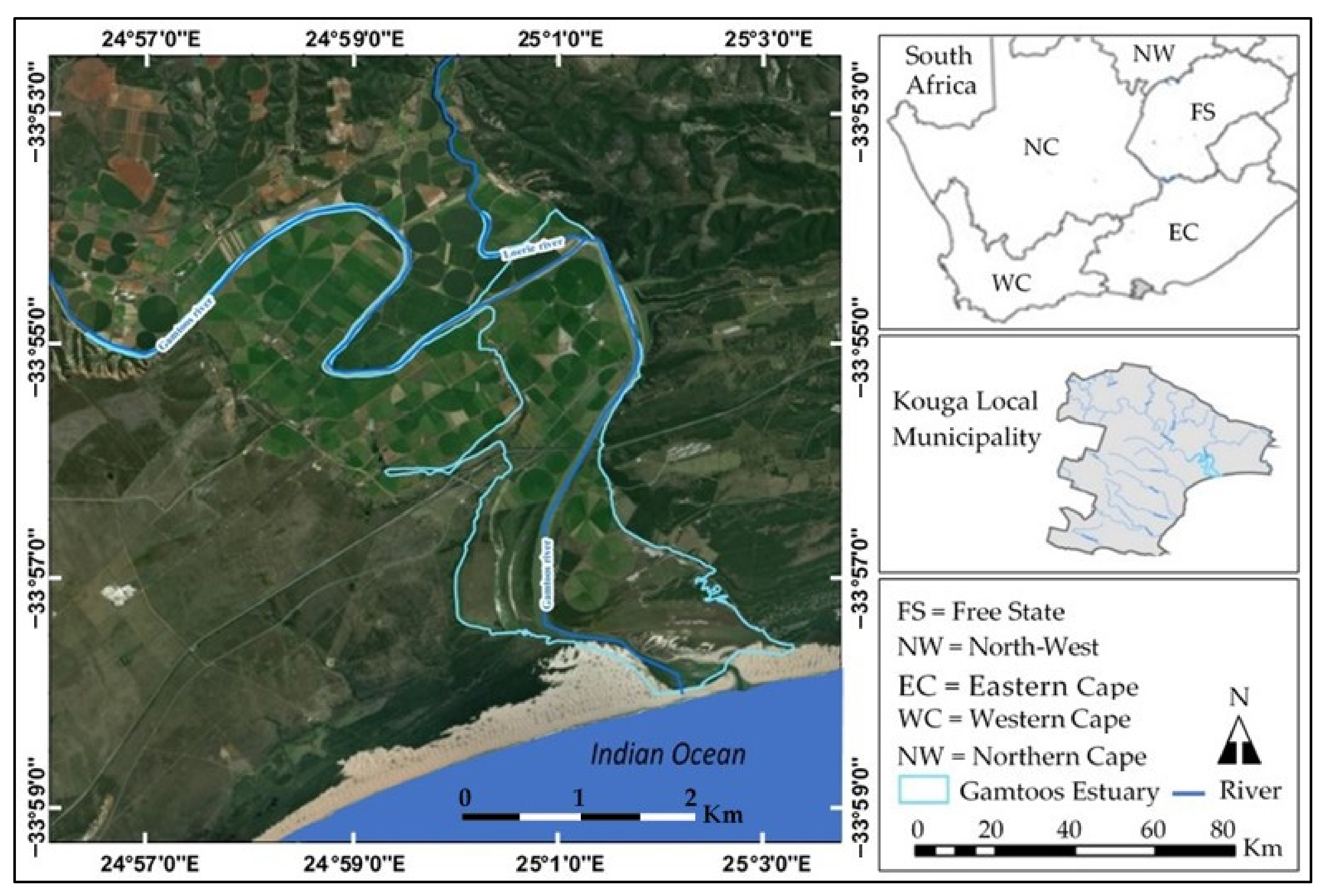
Figure 2.
Annual rainfall in Gamtoos River Estuary (a) and deviation from the mean (b): 1990–2017.
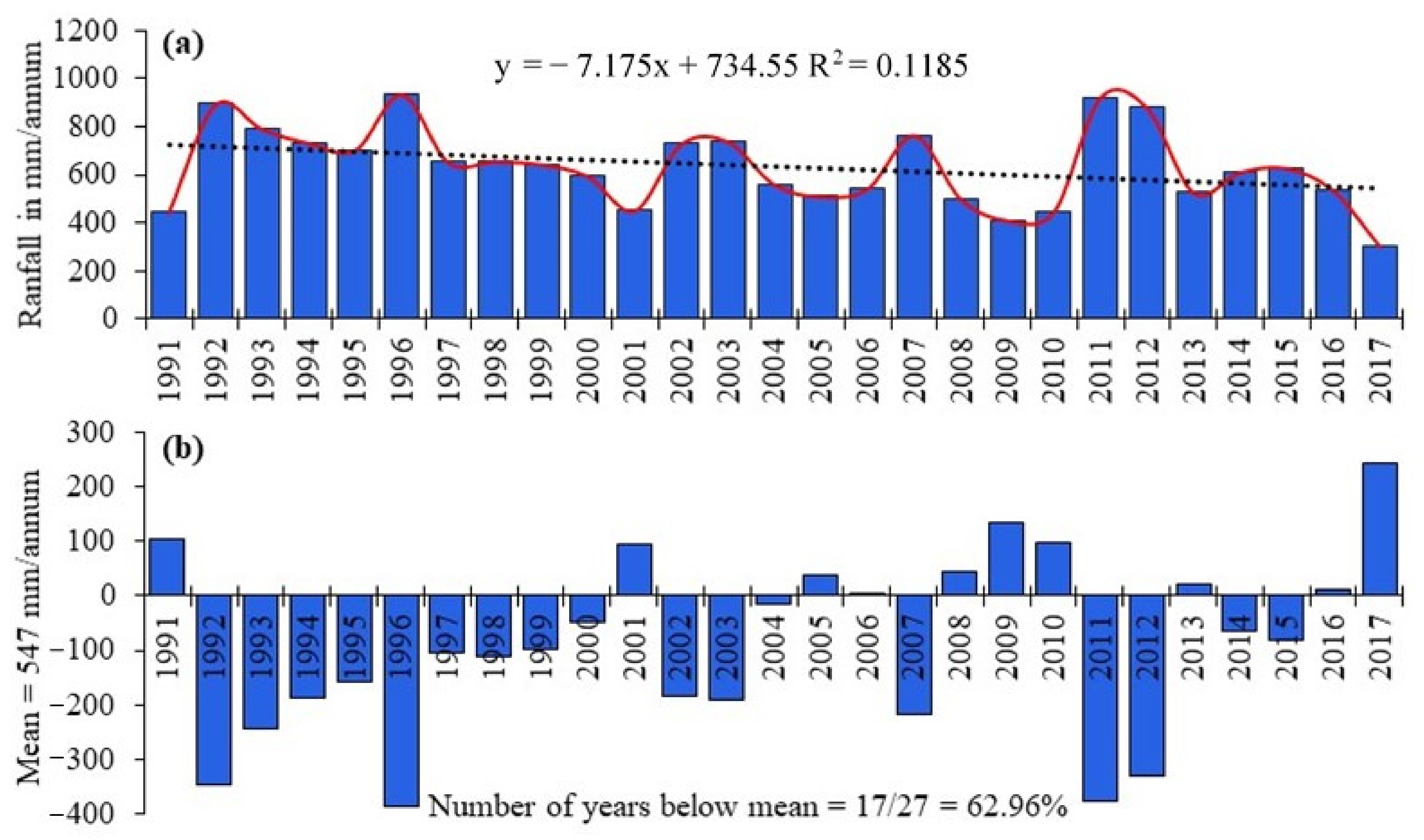
Figure 3.
Illustration of how Google Earth was used to aid the identification of different cover types in satellite images. Where ![Sustainability 14 07859 i001]() denotes Satellite image and
denotes Satellite image and ![Sustainability 14 07859 i002]() denotes Geo-located roadside photographs. (A,B)—Selected features in the image targeted for confident identification. (C)—Roadside view of point (A) in satellite image, Nov 2009. 33.924861S; 25.075820E. (D)—Roadside view of point (B) in image, Nov 2009. 33,921407S; 25.077065E. Link to source: [66].
denotes Geo-located roadside photographs. (A,B)—Selected features in the image targeted for confident identification. (C)—Roadside view of point (A) in satellite image, Nov 2009. 33.924861S; 25.075820E. (D)—Roadside view of point (B) in image, Nov 2009. 33,921407S; 25.077065E. Link to source: [66].
 denotes Satellite image and
  denotes Geo-located roadside photographs. (A,B)—Selected features in the image targeted for confident identification. (C)—Roadside view of point (A) in satellite image, Nov 2009. 33.924861S; 25.075820E. (D)—Roadside view of point (B) in image, Nov 2009. 33,921407S; 25.077065E. Link to source: [66].
Figure 3.
Illustration of how Google Earth was used to aid the identification of different cover types in satellite images. Where ![Sustainability 14 07859 i001]() denotes Satellite image and
denotes Satellite image and ![Sustainability 14 07859 i002]() denotes Geo-located roadside photographs. (A,B)—Selected features in the image targeted for confident identification. (C)—Roadside view of point (A) in satellite image, Nov 2009. 33.924861S; 25.075820E. (D)—Roadside view of point (B) in image, Nov 2009. 33,921407S; 25.077065E. Link to source: [66].
denotes Geo-located roadside photographs. (A,B)—Selected features in the image targeted for confident identification. (C)—Roadside view of point (A) in satellite image, Nov 2009. 33.924861S; 25.075820E. (D)—Roadside view of point (B) in image, Nov 2009. 33,921407S; 25.077065E. Link to source: [66].
denotes Satellite image and denotes Geo-located roadside photographs. (A,B)—Selected features in the image targeted for confident identification. (C)—Roadside view of point (A) in satellite image, Nov 2009. 33.924861S; 25.075820E. (D)—Roadside view of point (B) in image, Nov 2009. 33,921407S; 25.077065E. Link to source: [66].
Figure 4.
Sen Slope Estimates for land cover types that were computed by performing the M–K test in Excel.
Figure 4.
Sen Slope Estimates for land cover types that were computed by performing the M–K test in Excel.


Table 1.
Acquisition dates and characteristics of the SPOT images and aerial photographs that were used.
Table 1.
Acquisition dates and characteristics of the SPOT images and aerial photographs that were used.
| Satellite Images | Aerial Photographs | ||||
|---|---|---|---|---|---|
| Sensor | Date Acquired | Spectral Bands | Resolution | Cloud Cover | Date Acquired |
| SPOT 2 | 26/07/1991 | B1, B2, B3. | 22.01 m | <5% | 06/05/2013—Tc |
| SPOT 4 | 31/08/2000 | B1, B2, B3. | 21.58 m | 0% | 27/06/2003—Pan |
| SPOT 5 | 11/03/2009 | B1, B2, B3. | 11.91 m | <5% | 05/07/1994—Pan |
| SPOT 7 | 19/07/2017 | B1, B2, B3. | 5.63 m | <5% | 17/05/1980—Pan |
Table 2.
Adjusted annual rainfall (AAR) that was received in the 12 months before each image was acquired.
Table 2.
Adjusted annual rainfall (AAR) that was received in the 12 months before each image was acquired.
| Year | 1991 | 2000 | 2009 | 2017 |
|---|---|---|---|---|
| * | 08/1990–07/1991 | 07/1999–08/2000 | 02/2008–03/2009 | 08/2016–07/2017 |
| AAR: mm | 417.9 | 612.5 | 477.4 | 326.8 |
* Calendar months of which rainfall was used to calculate adjusted annual rainfall: AAR.
Table 3.
Illustration of how classification accuracy assessment was conducted based the SPOT 2000 image map output.
Table 3.
Illustration of how classification accuracy assessment was conducted based the SPOT 2000 image map output.
| (a) | Ba | Veg | Sw | Ca | Nc | Total | PA% | UA% | |
| Ba | 12 | 0 | 0 | 1 | 1 | 14 | 92.86 | 81.25 | |
| Veg | 0 | 21 | 1 | 0 | 1 | 23 | 82.61 | 90.48 | |
| Sw | 0 | 2 | 10 | 0 | 0 | 12 | 83.33 | 76.92 | |
| Cl | 1 | 0 | 0 | 12 | 1 | 14 | 78.57 | 91.66 | |
| Nc | 1 | 0 | 0 | 1 | 10 | 12 | 83.33 | 76.92 | |
| Total | 14 | 23 | 11 | 14 | 13 | 75 | |||
| PA = producer accuracy, UA = user accuracy, OA = sum of diagonal entries ÷ total = (65 ÷ 75) = 0.8667 = 86.7% (Ba = bare area, Veg = vegetation, Sw = surface water, Ca = cultivated land, Nc = noncultivated land) | |||||||||
| (b) Matrix produced in calculating the K statistic and explanation of how this was performed | |||||||||
| 196 | 322 | 154 | 196 | 182 | Explanation of calculations | ||||
| 322 | 529 | 253 | 322 | 299 | The first figure in Table (b) (196) is calculated by multiplying the total for bare area in Table (a) (14) with the horizontal row total for bare area in Table (a), i.e., 14 × 14 = 196. The remaining figures are calculated likewise. | ||||
| 168 | 276 | 132 | 168 | 156 | |||||
| 196 | 322 | 154 | 196 | 182 | |||||
| 168 | 276 | 132 | 168 | 156 | |||||
| Total | 1050 | 1725 | 825 | 1050 | 975 | ||||
| Grand total (sum of totals) = 5625 | |||||||||
Table 4.
Percentage compositions and percentage changes in the spatial distributions of land cover types that were mapped.
Table 4.
Percentage compositions and percentage changes in the spatial distributions of land cover types that were mapped.
| Cover Type | Percentage Composition | Percentage Change | ||||||
|---|---|---|---|---|---|---|---|---|
| 1991 | 2000 | 2009 | 2017 | A | B | C | D | |
| Bare area | 12.95 | 21.87 | 9.65 | 16.43 | 8.92 | −12.22 | 6.78 | 3.48 |
| Vegetation | 39.97 | 32.74 | 41.64 | 38.01 | −7.23 | 8.90 | −3.63 | −1.96 |
| Surface water | 7.11 | 12.65 | 7.06 | 7.55 | 5.54 | −5.59 | 0.49 | 0.44 |
| Cultivated land | 14.26 | 23.84 | 20.95 | 20.25 | 9.58 | −2.89 | −0.70 | 5.99 |
| Noncultivated land | 25.71 | 8.90 | 20.69 | 17.77 | −16.81 | 11.79 | −2.92 | −7.94 |
| Total area (ha) | 1736.4 | 1736.4 | 1736.4 | 1736.4 | − | − | − | − |
Percentage change labels: A: 1991–2000; B: 2000–2009; C: 2009–2017; D: 1991–2017.
Table 5.
Trend coefficients based on compositions of the cover types that were mapped and correlations between their percentage compositions with adjusted annual rainfall (AAR).
Table 5.
Trend coefficients based on compositions of the cover types that were mapped and correlations between their percentage compositions with adjusted annual rainfall (AAR).
| Cover Types | Trend Coefficient | R2 | SSE | p (σ 0.05) |
|---|---|---|---|---|
| Bare area: (Ba) | y = −0.1797x + 15.675 | 0.002 | −0.025 | * 1.0000 |
| Vegetation: (Veg) | y = 0.3029x + 37.334 | 0.010 | 0.009 | ** 1.0000 |
| Surface water: (Sw) | y = −0.4261x + 9.657 (Ɲ) | 0.041 | 0.007 | ** 1.0000 |
| Cultivated land: (Ca) | y = 1.5061x + 16.059 | 0.234 | 0.071 | ** 1.0000 |
| Noncultivated land: (Nca) | y = −1.2032x + 21.275 | 0.049 | −0.292 | * 0.7341 |
| AAR: (1991, 2000, 2009, 2017) | y = −40.84x + 560.75 | 0.194 | −9.258 | * 0.7341 |
| Long-term rainfall: 1991–2017 | y = −7.175x + 734.55 | 0.119 | −11.130 | *** 0.0411 |
| Correlations between AAR and different cover types at σ = 0.05, Critical R = 0.805 | ||||
| * AAR & Ba = 0.453816 | AAR & Sw = ***0.813709 | AAR & Nca = **−0.643962 | ||
| ** AAR & Veg = −0.592468 | AAR & Ca = 0.560341 | *** Significant positive | ||
No trend if p is > 0.05). (Ɲ) = false negative trend. Negative SSE = declining trend and vice versa. * = insignificant decrease. ** = insignificant increase. *** = significant decrease.
Publisher’s Note: MDPI stays neutral with regard to jurisdictional claims in published maps and institutional affiliations. |
© 2022 by the authors. Licensee MDPI, Basel, Switzerland. This article is an open access article distributed under the terms and conditions of the Creative Commons Attribution (CC BY) license (https://creativecommons.org/licenses/by/4.0/).
Share and Cite
MDPI and ACS Style
Ndude, M.A.; Gwena, K.R.; Hamandawana, H. The Nature, Causes and Extent of Land cover Changes in Gamtoos River Estuary, Eastern Cape Province, South Africa: 1991–2017. Sustainability 2022, 14, 7859. https://doi.org/10.3390/su14137859
AMA Style
Ndude MA, Gwena KR, Hamandawana H. The Nature, Causes and Extent of Land cover Changes in Gamtoos River Estuary, Eastern Cape Province, South Africa: 1991–2017. Sustainability. 2022; 14(13):7859. https://doi.org/10.3390/su14137859
Chicago/Turabian StyleNdude, Mhlanganisi Africa, Kudzanai Rosebud Gwena, and Hamisai Hamandawana. 2022. "The Nature, Causes and Extent of Land cover Changes in Gamtoos River Estuary, Eastern Cape Province, South Africa: 1991–2017" Sustainability 14, no. 13: 7859. https://doi.org/10.3390/su14137859
Note that from the first issue of 2016, this journal uses article numbers instead of page numbers. See further details here.