Applying the Random Forest Method to Improve Burner Efficiency

Abstract

Fuel power plants are one of the main sources of pollutant emissions, so special attention should be paid to improving the efficiency of the fuel combustion process. The mathematical modeling of processes in the combustion chamber makes it possible to reliably predict and find the best dynamic characteristics of the operation of a power plant, in order to quantify the emission of harmful substances, as well as the environmental and technical and economic efficiency of various regime control actions and measures, and the use of new types of composite fuels. The main purpose of this article is to illustrate how machine learning methods can play an important role in modeling and predicting the performance and control of the combustion process. The paper proposes a mathematical model of an unsteady turbulent combustion process, presents a model of a combustion chamber with a combined burner, and performs a numerical study using the STAR-CCM+ multidisciplinary platform. The influence of various input indicators on the efficiency of burner devices, which is evaluated by several parameters at the output, is investigated. In this case, three possible states of the burners are assumed: optimal, satisfactory and unsatisfactory.

1. Introduction

When burning fuel in combustion devices, it is necessary to ensure that the most economical mode is maintained to reduce the emission of pollutants. When organizing the operation mode of the combustion devices of power plants, it is required to organize the influence of heat and mass transfer processes and aerodynamics on the ongoing chemical reactions in such a way as to ensure the most complete and environmentally friendly fuel combustion [1,2]. At high temperatures, a certain amount of toxic nitrogen oxides is formed in the combustion chamber in the form of $NO$, $N{O}_2$, $N_2{O}_4$, $N_2{O}_5$, etc., along with emissions of $S{O}_2$, $C{O}_2$ [3,4]. In calculations, it is conditionally assumed that nitrogen oxides emitted into the atmosphere consist only of $N{O}_2$.

An increase in the installed unit capacity of the boilers makes it necessary to speed up the combustion processes in order to reduce the structural dimensions of the boiler. The main pollutant during the combustion of natural gas in power plants are thermal nitrogen oxides, the main indicator of the formation intensity of which is the temperature in the zone of active combustion [5,6]. To reduce $N{O}_X$ emissions with flue gases, a number of measures are used, including furnace sectioning, flue gas recirculation, air temperature reduction, moisture injection into the combustion zone, staged combustion, etc. It will be 20 °C by 2050 by limiting the growth of global energy consumption to no more than 25% and doubling harmful emissions; experts of the International Energy Agency indicate, to a large extent with the improvement of fuel energy technologies, an increase in the share of energy production from renewable sources and the development of distributed energy.

The furnace device is a complex gas–steam–water heat exchange device. The basis of the combustion process in the furnace is the chemical reactions of oxygen with combustible fuel elements. These processes take place under difficult conditions, creeping up on chemical processes [7]. The modeling of furnace processes has been carried out for more than half a century, while it is practically impossible to conduct direct furnace simulation of furnace processes due to the need for simultaneous simulation of combustion, aerodynamics, heat and mass transfer processes [8]. Secondary vortex currents may occur in the combustion chamber. For more accurate modeling, it is necessary to take into account the turbulent and molecular diffusion of the initial components and reaction products in the gas flow. In this regard, approximate modeling is possible. In furnace devices, the process of convective mixing is decisive, and is largely determined by the design of the burners.

The study of the combustion process and heat transfer in the furnace space is an extremely important task, which is the subject of many works by such authors as Bin Xu, Dewallefa P., Domoto K., Hidetoshi A., June Wang, Rezwanul K. and Sartor K. [9,10,11].

The processes of chemical kinetics determine the rate of the reaction at which the formation of combustion products occurs, as described by the Arrhenius equation. For the calculated reaction rate in the framework of the turbulent vortex decay model, the Eddy Dissipation Model takes the minimum of them. However, since all reactions are characterized by the same mixing rate, this model can only be used with a single-stage (reagent-product) or two-stage (reagent-intermediate-product) global reaction [12].

An alternative approach to describing the combustion process of swirling flows is the simulation of transport equations (convection, diffusion), which makes it possible to perform calculations for multicomponent fuel mixtures with acceptable accuracy. Külsheimer C. investigates the effect of periodic excitation of a mass flow rate variable in frequency and amplitude on the isothermal flow field and the characteristics of the flame of swirl burners with different swirling intensity. The results demonstrate that the minimum level of excitation of the mass flow rate for the formation of vortices decreases hyperbolically with an increase in the pulsation frequency and the characteristic Strouhal number, respectively [13].

Galley D. proposed a mathematical model, with the help of which he conducted a study of an unsteady turbulent gas flow, followed by combustion in a combustion chamber. For the completeness of fuel combustion and to achieve maximum efficiency during fuel combustion, the flow swirl was modeled [14].

To obtain accurate results of aerodynamic and thermochemical processes in the furnace space with calculations of turbulent, reactive and heat flows for various boiler operating modes, CFD modeling is used, which allows for optimizing operating modes [15,16,17]. Gianmarco Aversano, Marco Ferrarotti and Alessandro Parente developed a reduced order model based on CFD simulations and performed 3D simulations with detailed chemistry covering a wide range of operating conditions in terms of fuel composition (methane hydrogen mixtures from pure methane to pure hydrogen) [18].

Power boilers must be characterized by high flexibility and, when operating at a technical minimum, the combustion process must be stable. Thus, Henrik B. obtained a fairly good agreement between the values obtained for the power boiler using CFD simulations with the values obtained using analytical models. He demonstrated the stability of combustion at the minimum load of the boiler and analyzed the value of $N{O}_X$ emission when the flame moved upwards [19]. Currently, to improve the technical and economic indicators and environmental characteristics of power boilers, efficient furnace devices are being developed based on low-temperature vortex fuel combustion technology, as well as vortex combustion in boiler furnaces with advanced supercritical steam parameters [20].

A number of authors have carried out studies of the influence of the design of burners on the emission of pollutants using mathematical modeling, which confirmed the effect of changing the supply of oxidizer and nozzle geometry on the intensity of the mixing of gaseous media and the formation of emissions. M. Rimar, Jan Kizek and Andrii Kulikov, using computer simulation, confirmed the effect of changing the supply of oxidizer and the geometry of air nozzles on the intensity of the mixing of gaseous media and the formation of emissions. The introduction of a separating insert into the air nozzle made it possible to intensify the mixing of gaseous media. Zheltukhina E. considered the formation of toxic compounds and the possibility of modeling combustion processes to reduce them [21,22]. $N{O}_X$ emissions can be controlled by limiting the amount of available oxygen that can combine with nitrogen to form nitric oxide ($NO$). The optimum operating point for minimizing $N{O}_X$ emissions may vary depending on the combustion process, including load conditions, equipment condition, fuel type and process conditions. The design of the burner and its modes of operation largely determine the intensity of flame ignition, the conditions and rate of mixing of the fuel with the oxidizer and the maximum temperature level in the combustion core. By changing the design of the burner, it is possible to influence these parameters and, thereby, reduce the formation of $N{O}_X$ from 30 to 60% without worsening the combustion process at reduced capital and operating costs [23].

Another widely used method of combating the emission of harmful substances is flue gas recirculation (FGR) [24,25,26]. The main share of $N{O}_X$ is formed in the area of a high temperature of the combustion flame (more than 1500 °C), and then, under the action of a vortex gas flow, it moves throughout the entire furnace volume. When about 10% of the flue gases are added to the flame, the temperature is reduced by about 7%. It is noted that recirculating the flue gas in the fuel stream, i.e., fuel-induced recirculation (FIR), can improve significantly improved $N{O}_X$ reduction per unit mass of recycled gas compared to conventional recirculation. The effect of internal flue gas recirculation on $N{O}_X$ and $S{O}_X$ emissions from boilers was also considered. When studying the operation of a low-emission burner, a number of researchers found that despite the fact that 1% flue gas recirculation reduces the boiler efficiency by 0.03–0.06%, at maximum boiler load and 13% recirculation, a reduction in $N{O}_X$ emissions by 44.5% can be achieved, up to 90 mg/m${}^3$ [27,28,29]. Jun Li and Xiaolei Zhang et al. considered the effect of internal flue gas recirculation on $N{O}_X$ and $S{O}_X$ emissions in a co-firing boiler. Internal flue gas recirculation is an effective way to reduce $S{O}_X$ emissions, and an increase in the recirculation ratio leads to a significant reduction in $N{O}_X$ emissions; however, $S{O}_X$ increased slightly [30]. Mohsen Abdelaal and Medhat El-Riedy et al. found that the flame remains stable up to a recirculation level of 40%, but the temperature decreases by about 25%, and the $S{O}_X$ content decreases from 90 to 5 ppm [31]. In this case, combustion instability can be associated with the level of $N{O}_X$ emissions in premix burners [32]. Ehsan Houshfar and colleagues used two different compositions of recirculating flue gases: $C{O}_2$ and $C{O}_2$ + $NO$ [33].

FGR is being actively introduced to reduce emissions in biofuel boilers of various capacities [34,35,36]. Much attention is currently paid to the use of hydrogen, methane-hydrogen fractions, fuel mixtures based on landfill gases and thermal decomposition products of industrial and municipal waste as fuel in power plants [37,38,39]. Thus, Yue Xin, Ke Wang and colleagues found that the optimal proportion of mixing natural gas and hydrogen is 24.7% [40].

Simulation and study of the processes of the combined combustion of composite fuels will make it possible to become closer to the transition to environmentally friendly and resource-saving energy. Composite fuel is a mechanical mixture of combustibles (including organic fuels), and in some cases combustible and non-combustible substances, which has new thermal properties compared to the properties of the original combustibles [41]. Known low-emission combustion technologies are based on the use of synthesis gas as a fuel. J. Sidey, in his study, considered the structure and stability of the flame of a dual-fuel flame and the analysis of experimental data to verify the model. Visualization results demonstrate the structure of the internal flame along the jet in the form of a hollow cone and the structure of the external flame in the shear layer between the ring oxidizer and the internal recirculation zone above the shedder [42].

The processes of the combined combustion of natural gas mixed with synthesis gas largely depend on the preparation of the air-fuel mixture in the burner and directly in the flame. The preparation of the air-fuel mixture is especially relevant in connection with the phenomena of the breakdown and flashback of the flame. To ensure a stable position in the combustion space of the ignition zone, i.e., flame front, the mixture to the ignition zone should be supplied at a speed equal to the speed of flame propagation [43].

Considering this review, we come to the conclusion that, due to the complexity of the mathematical formulation of the turbulent combustion problem, which includes a system of coupled nonlinear non-stationary differential equations of motion, energy and chemical kinetics equations, the solution to the problem of high-precision modeling and prediction of physical and chemical processes in combustion chambers can only be obtained based on mathematical modeling [44]. At the same time, the methodological aspect of the problem is associated with the development of effective mathematical methods for modeling the processes of turbulent exchange and chemical kinetics in the combustion chamber, which ensure the convergence and sufficient accuracy of the obtained numerical solution at an acceptable cost of computer time. Solving the problem of high-temperature gas motion is a labor-intensive task that requires significant computational resources. One of the problems of solvers in a high-fidelity simulation can be resource intensive. Such tasks require the use of modern computing systems and machine learning technologies that optimize the cost of resources for the implementation of computational experiments [45].

The novelty of this work in machine learning is as follows: In testing several different methods for classifying the condition of the burners in order to select the best one; in the aggregation of these methods—in binary classification problems, this approach demonstrated a significant increase in the quality of training; in the study of the influence of various factors (the influence of correlation and the presence of outliers, the influence of random scattering, the share of the test sample, the influence of the number of cross-validation blocks on the quality of training (similar studies were carried out earlier, but to increase the efficiency of the burners, it is carried out for the first time).

2. Mathematical Modeling of the Efficiency of Burners

2.1. 3D Model of the Burner

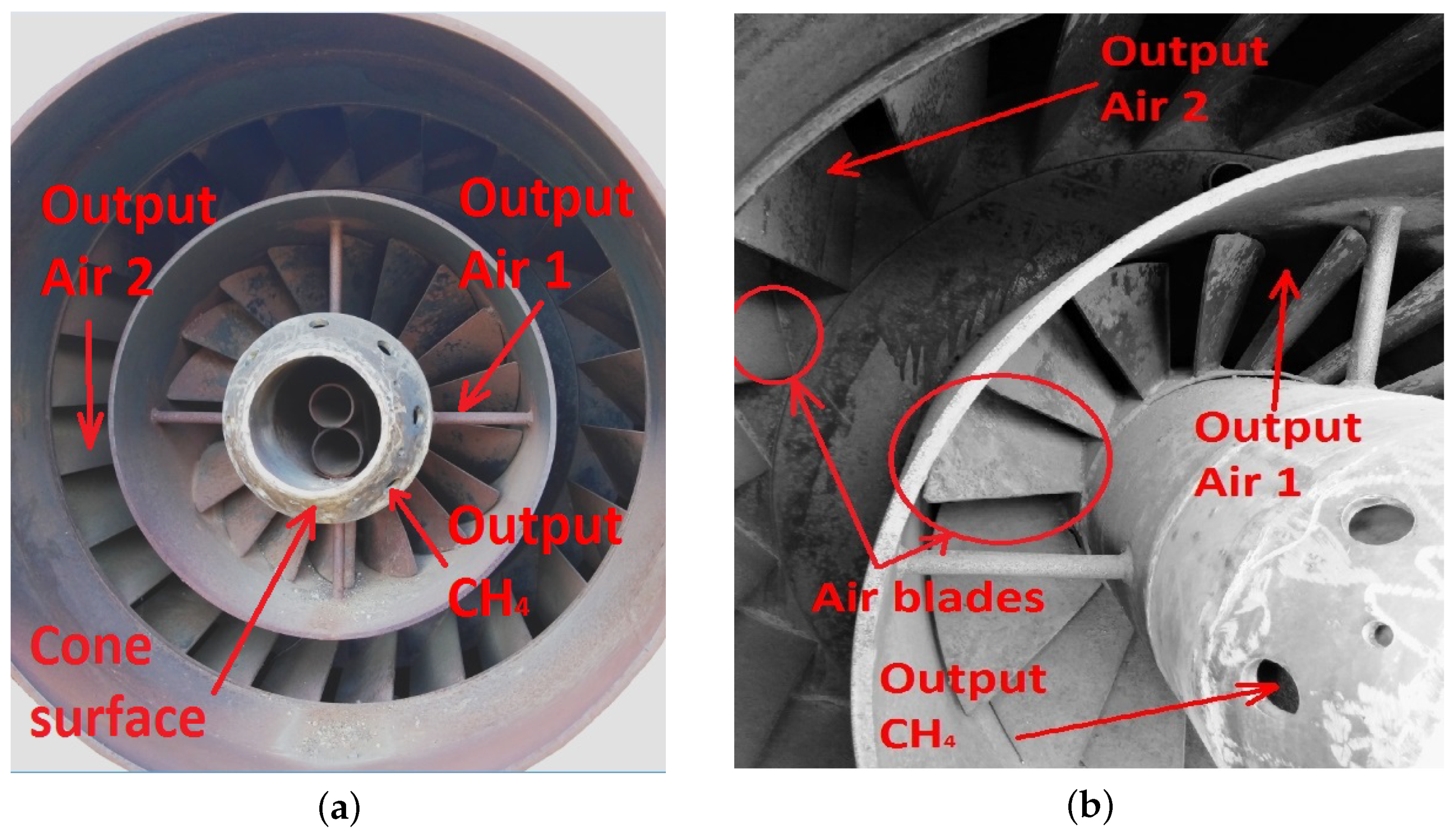
The multidisciplinary platform STAR-CCM+ was chosen for the numerical simulation of hydrocarbon fuel combustion, since it allows for solving problems of modeling turbulent flows, taking into account the chemical kinetics of reacting flows. This makes it possible to identify and analyze the relationship between the performance of the boiler plant and the emission of pollutants under various operating conditions. As a representative prototype for building a 3D model of the burner device (Figure 1), a modernized oil-gas burner based on GMU-45 (Figure 2) was selected.

To ensure acceptable air speeds when the burner is operating at low loads, the air channel in the outlet part is divided into internal and peripheral flows. Air flows before entering the burner embrasure pass swirling devices. The twisting of the air flow in the internal channel is carried out by an axial device. This unit has 18 fixed blades at an angle of 20° to the burner axis. The twisting of the air flow in the peripheral channel is carried out by a tangential swirler with 24 fixed blades set at an angle of 60° to the radius.

The burner has a central gas supply. Gas is supplied to the space between the central diameter of 219 × 6 mm and the outer diameter of 325 × 9 mm pipes. On the side of the furnace, the gas collector ends with a truncated cone, in which holes are drilled. The gas exits the holes at an angle to the axis of the air flow.

When constructing a 3D model of the burner, the design parameters of the prototype were used, including overall dimensions, the number of elements of the swirling apparatus, flow swirl angles, rows and the number of gas outlets.

2.2. Mathematical Model of Gas Dynamics

To simulate the combustion process of a swirling fuel-air unsteady flow, a mathematical model is proposed, including:

Continuity equation:

$$\begin{array}{c}\hfill \frac{\partial \rho }{\partial t}+\frac{\partial }{\partial x}\left(\rho u\right)+\frac{\partial }{\partial r}\left(\rho \upsilon \right)+\frac{1}{r}\frac{\partial }{\partial \theta }\left(\rho w\right)=0.\end{array}$$

(1)

Motion equation:

• x-component

  $$\begin{array}{c}\hfill \frac{\partial }{\partial t}\left(\rho u\right)+u\frac{\partial }{\partial x}\left(\rho u\right)+\upsilon \frac{\partial }{\partial r}\left(\rho u\right)+\frac{w}{r}\frac{\partial }{\partial \theta }\left(\rho u\right)\\ \hfill =-\frac{\partial P}{\partial x}+\mu [\frac{{\partial }^{2}u}{\partial x^2}+\frac{1}{r}\frac{\partial }{\partial r}(r\frac{\partial u}{\partial r}+\frac{1}{r^2}\frac{{\partial }^{2}u}{\partial {\theta }^2}]\\ \hfill +\left[-\frac{\partial \left(\overline{\rho {u^{\prime }}^2}\right)}{\partial x}-\frac{\partial \left(\overline{\rho u^{\prime }{\upsilon }^{\prime }}\right)}{\partial r}-\frac{1}{r}\frac{\partial \left(\overline{\rho u^{\prime }{w}^{\prime }}\right)}{\partial \theta }\right]\end{array}$$

  (2)
• r-component

  $$\begin{array}{c}\hfill \frac{\partial }{\partial t}\left(\rho \upsilon \right)+u\frac{\partial }{\partial x}\left(\rho \upsilon \right)+\upsilon \frac{\partial }{\partial r}\left(\rho \upsilon \right)+\frac{w}{r}\frac{\partial }{\partial \theta }\left(\rho \upsilon \right)-\frac{w^2}{r}\\ \hfill =-\frac{\partial P}{\partial r}+\mu \left[\frac{{\partial }^2\upsilon }{\partial x^2}+\frac{1}{r}\frac{\partial }{\partial r}\left(r\frac{\partial \upsilon }{\partial r}\right)+\frac{1}{r^2}\frac{{\partial }^2\upsilon }{\partial {\theta }^2}-\frac{\upsilon }{r^2}-\frac{2}{r^2}\frac{\partial w}{\partial \theta }\right]\\ \hfill +\left[-\frac{\partial \left(\overline{\rho u^{\prime }{\upsilon }^{\prime }}\right)}{\partial x}-\frac{\partial \left(\overline{\rho {{\upsilon }^{\prime }}^2}\right)}{\partial r}-\frac{1}{r}\frac{\partial \left(\overline{\rho {\upsilon }^{\prime }{w}^{\prime }}\right)}{\partial \theta }\right]\end{array}$$

  (3)
• $\theta$-component

  $$\begin{array}{c}\hfill \frac{\partial }{\partial t}\left(\rho w\right)+u\frac{\partial \left(\rho w\right)}{\partial x}+\upsilon \frac{\partial \left(\rho w\right)}{\partial r}+\frac{w}{r}\frac{\partial \left(\rho w\right)}{\partial \theta }+\frac{\upsilon w}{r}\\ \hfill =-\frac{1}{r}\frac{\partial P}{\partial \theta }+\mu \left[\frac{{\partial }^{2}w}{\partial x^2}+\frac{1}{r}\frac{\partial }{\partial r}\left(r\frac{\partial w}{\partial r}\right)+\frac{1}{r^2}\frac{{\partial }^{2}w}{\partial {\theta }^2}+\frac{2}{r^2}\frac{\partial \upsilon }{\partial \theta }-\frac{w}{r^2}\right]\\ \hfill +\left[-\frac{\partial \left(\overline{\rho u^{\prime }{w}^{\prime }}\right)}{\partial x}-\frac{\partial \left(\overline{\rho {\upsilon }^{\prime }{w}^{\prime }}\right)}{\partial r}-\frac{1}{r}\frac{\partial \left(\overline{\rho {w^{\prime }}^2}\right)}{\partial \theta }\right]\end{array}$$

  (4)

  where $u,v,w$—velocity components in the $x,r,\theta$ directions, respectively; $\rho$—density [kg/m${}^3$]; P—pressure [Pa]; $\mu$—dynamic viscosity [Pa · s]; Reynolds stress – (–$\overline{\rho {u\prime }^2}$, –$\overline{\rho {\upsilon \prime }^2}$, –$\overline{\rho {w\prime }^2}$, –$\overline{\rho u^{\prime }}$, –$\overline{\rho {\upsilon }^{\prime }}$, –$\overline{\rho w^{\prime }}$); t—time [c]; $x,r,\theta$—cylindrical coordinates.

Energy equation:

$$\begin{array}{c}\hfill \rho c_p\left(\frac{\partial T}{\partial t}+\upsilon \frac{\partial T}{\partial r}+\frac{w}{r}\frac{\partial T}{\partial \theta }+u\frac{\partial T}{\partial x}\right)=div\left[\left(\lambda +\frac{c_p{\mu }_T}{P{r}_T}\right)gradT-\sum _j{h}_j{J}_j\right]+S_h,\end{array}$$

(5)

where

$$\begin{array}{c}\hfill div=\frac{\partial }{\partial x}+\frac{\partial }{\partial r}+\frac{1}{r}\frac{\partial }{\partial \theta },\end{array}$$

(6)

$$\begin{array}{c}\hfill h=\sum _j{Y}_j{h}_j+\frac{P}{\rho },h_j={\int }_{T_{ref}}^T{c}_{p,j}dT,T_{ref}=298.15\mathrm{K}.\end{array}$$

(7)

where ${\mu }_T$—coefficient turbulent viscosity [Pa · s]; T—temperature [K]; $\lambda$—coefficient of thermal conductivity [W/m · K]; $S_h$—includes the heat of the chemical reaction, and any other volumetric heat sources are specified; $c_p$—specific heat (J/kg · k); $P{r}_T$—turbulent Prandtl number; $Y_j$—mass fraction of the species j.

Mass diffusion $J_j$ is calculated using the following form:

$$\begin{array}{c}\hfill J_j=-\left(\rho D_{i,m}+\frac{{\mu }_T}{S{c}_T}\right)div{Y}_j.\end{array}$$

(8)

where $D_{i,m}$—mass diffusion coefficient for type i in the mixture; $S{c}_T$—the turbulent Schmidt number is 0.7.

Let us express the turbulent Prandtl number $P{r}_T$ by the dependence:

$$\begin{array}{c}\hfill P{r}_T=\frac{\overline{u^{\prime }{\upsilon }^{\prime }}}{du/dr}\frac{dT/dr}{\overline{T^{\prime }{\upsilon }^{\prime }}}=\frac{u^{\prime }}{T^{\prime }}\frac{R_{u\upsilon }}{R_{T\upsilon }}\frac{\frac{dT}{dr}}{\frac{du}{dr}}\end{array}$$

(9)

where $T^{\prime }$—RMS flow temperature ripple; $\overline{T^{\prime }{\upsilon }^{\prime }}$, $\overline{u^{\prime }{\upsilon }^{\prime }}$—correlation functions; $R_{u\upsilon }$, $R_{T\upsilon }$—correlation coefficients between pulsations $u^{\prime }$, ${\upsilon }^{\prime }$ and $T^{\prime }$, ${\upsilon }^{\prime }$ respectively. Pulsations $u^{\prime }$, $T^{\prime }$ at an arbitrary point of a thermally unsteady boundary layer, in accordance with the mixing path model, are expressed by the relations:

$$\begin{array}{c}\hfill u^{\prime }=l\frac{du}{dr},T^{\prime }=l_T\frac{dT}{dr}\end{array}$$

(10)

where $l,l_T$—the length of the mixing path for velocity and temperature fluctuations, respectively.

For combustion modeling, the basis of the non-premix combustion approach is that the instantaneous thermochemical state of the flow is related to a conservative scalar variable called the mixture fraction. The mixture fraction f can be written as follows:

$$\begin{array}{c}\hfill f=\frac{\left[Y_g-\widehat{s}{Y}_{O_2}\right]-{\left[Y_g-\widehat{s}{Y}_{O_2}\right]}_2}{{\left[Y_g-\widehat{s}{Y}_{O_2}\right]}_1-{\left[Y_g-\widehat{s}{Y}_{O_2}\right]}_2}\end{array}$$

(11)

where $\widehat{s}$—mass ratio of fuel to air ($\widehat{s}$=$\frac{\left(m_{{\mathrm{CH}}_4}\right)}{{(m}_{O_2})}$); $Y_g$ and $Y_{O_2}$ represent, respectively, the values of the mass fractions of fuel and $O_2$ at the outlet of the fuel injectors (indicated by number 1) and air (indicated by number 2).

The species conservation equations solved for each chemical reduce to a single mixture fraction conservation equation:

$$\begin{array}{c}\hfill \frac{\partial }{\partial t}\left(\rho \tilde{f}\right)+\frac{\partial }{\partial x_i}\left(\rho u_i\tilde{f}\right)=\frac{\partial }{\partial x_i}\left(\frac{{\mu }_T}{{\sigma }_t}\frac{\partial \tilde{f}}{\partial x_i}\right),\end{array}$$

(12)

where $u_i$—corresponding velocity component [m/s]; $x_i$—corresponding coordinate component [m].

Moreover, the resolution of the additional equation for the variance of the mixture fraction $\widetilde{f^{{}^{\prime }2}}$:

$$\begin{array}{c}\hfill \frac{\partial }{\partial t}\left(\rho \widetilde{{f^{\prime }}^2}\right)+\frac{\partial }{\partial x_i}\left(\rho u_i\widetilde{{f^{\prime }}^2}\right)=\frac{\partial }{\partial x_i}\left(\frac{{\mu }_t}{0.85}\frac{\partial \widetilde{f^{{}^{\prime }2}}}{\partial x_i}\right)+2.86{\mu }_t{\left(\frac{\partial \tilde{f}}{\partial x_i}\right)}^2-2\rho \frac{ϵ}{k}\widetilde{f^{{}^{\prime }2}},\end{array}$$

(13)

where $k,ϵ$—turbulence kinetic energy [m${}^2$/s${}^2$] and its dissipation rate [m${}^2$/s${}^3$].

The k-$ϵ$ (Realizable) turbulence model was used to describe turbulence. The turbulence kinetic energy k and its dissipation rate $ϵ$ for an unsteady flow satisfy the following transfer equations:

$$\begin{array}{c}\hfill \frac{\partial }{\partial t}\left(\rho k\right)+\frac{\partial }{\partial x_i}\left(\rho k{u}_i\right)=\frac{\partial }{\partial x_i}\left[\left(\mu +\frac{{\mu }_t}{{\sigma }_k}\right)\frac{\partial k}{\partial x_j}\right]+G_k+G_b-\rho ϵ-Y_M+S_k,\end{array}$$

(14)

$$\begin{array}{c}\hfill \frac{\partial }{\partial t}\left(\rho ϵ\right)+\frac{\partial }{\partial x_i}\left(\rho ϵu_i\right)=\frac{\partial }{\partial x_i}\left[\left(\mu +\frac{{\mu }_t}{{\sigma }_{ϵ}}\right)\frac{\partial ϵ}{\partial x_j}\right]+\rho C_1{S}_{ϵ}-\rho C_2\frac{{ϵ}^2}{k+\sqrt{\nu ϵ}}+C_{1ϵ}\frac{ϵ}{k}{C}_{3ϵ}{G}_b+S_{ϵ},\end{array}$$

(15)

where

$$\begin{array}{c}\hfill C_1=max\left[0.43,\frac{\eta }{\eta +5}\right],C_{3ϵ}=tanh\left|\frac{\upsilon }{u}\right|,\\ \hfill eta=S\frac{k}{ϵ},{\sigma }_k=1,{\sigma }_{ϵ}=1.2,C_{1ϵ}=1.44,C_2=1.9,\end{array}$$

(16)

where ${\sigma }_k,{\sigma }_{ϵ}$—are the reciprocal effective Prandtl numbers for k and $ϵ$, respectively; $G_k$—source due to the mean velocity gradient; $G_b$—generation of kinetic energy of turbulence due to buoyancy; $Y_M$- represents the contribution of oscillating dilatation in compressible turbulence to the total scattering velocity; $S_k$, $S_{ϵ}$—user-defined sources; $C_{3ϵ}$—degree of buoyancy; $u,\upsilon$—velocity components along the x, y axes, respectively; $\eta$—dimensionless coordinate; S—mean strain rate tensor.

To simulate turbulent viscosity in the core, the following expression is defined:

$$\begin{array}{c}\hfill {\mu }_T=\rho C_{\mu }\frac{k^2}{ϵ},\end{array}$$

(17)

where $C_{\mu }$—empirical coefficient equal to $C_{\mu }$ = 0.09.

2.3. Border Conditions

The boundary conditions were set as follows:

-

On the walls:

$$\begin{array}{c}\hfill x\in \left(0,L\right):u\left(x,R,\theta \right)=0;\upsilon \left(x,R,\theta \right)=0;w\left(x,R,\theta \right)=0;T\left(x,R,\theta \right)=T_w.\\ \hfill R^{*}\in \left(r_B,R\right):u\left(x_0,R^{*},\theta \right)=0;\upsilon \left(x_0,R^{*},\theta \right)=0;w\left(x_0,R^{*},\theta \right)=0;T\left(x_0,R^{*},\theta \right)=T_w.\end{array}$$

(18)

-

Inlet:

$$\begin{array}{c}\hfill r\in \left(0,r_B\right):u\left(x_0,r^{*},\theta \right)=U_{air}+U_{fuel};\upsilon \left(x_0,r^{*},\theta \right)=0;w\left(x_0,r^{*},\theta \right)={\omega }_{air};\\ \hfill P\left(x_0,r^{*},\theta \right)=P_{air}+P_{fuel};T\left(x_0,r^{*},\theta \right)=T_{air}+T_{fuel}.\end{array}$$

(19)

-

Outlet:

$$\begin{array}{c}\hfill p\left(L,r,\theta \right)=0,r\in \left(0,R\right).\end{array}$$

(20)

2.4. Mesh Selection and Mesh Convergence Analysis

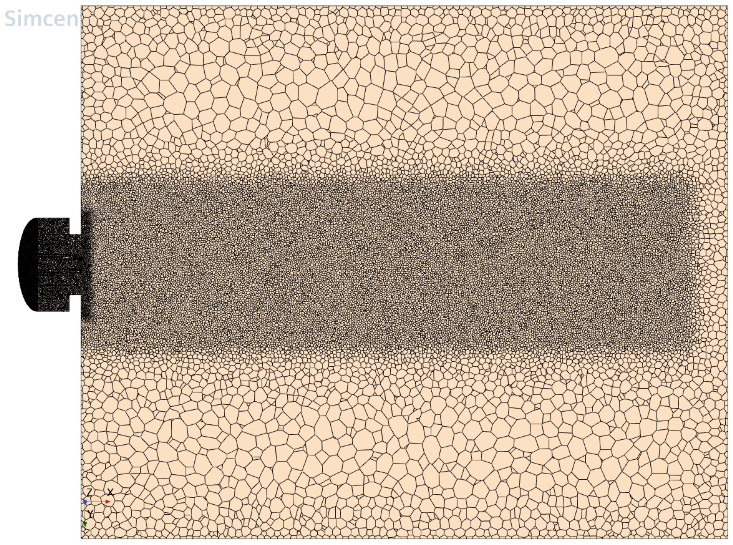
Using the 3D-CAD Models module, a combustion chamber with one combined burner was modeled. The generation of the computational grid was carried out using the Mesh module, a conformal grid was applied with the use of zonal thickening of grid elements.

Figure 3 and Figure 4 show examples of the computational grid for the burner and combustion zone. At this stage of research, the grid is divided into three zones: the first zone is a burner device in which mixing and swirling of methane-air mixture flows is carried out; the second zone is the most efficient zone in the center of the combustion chamber after exiting the burner, where the temperature and flame propagation speed are the highest compared to other areas; the third zone is the least effective zone compared to the others.

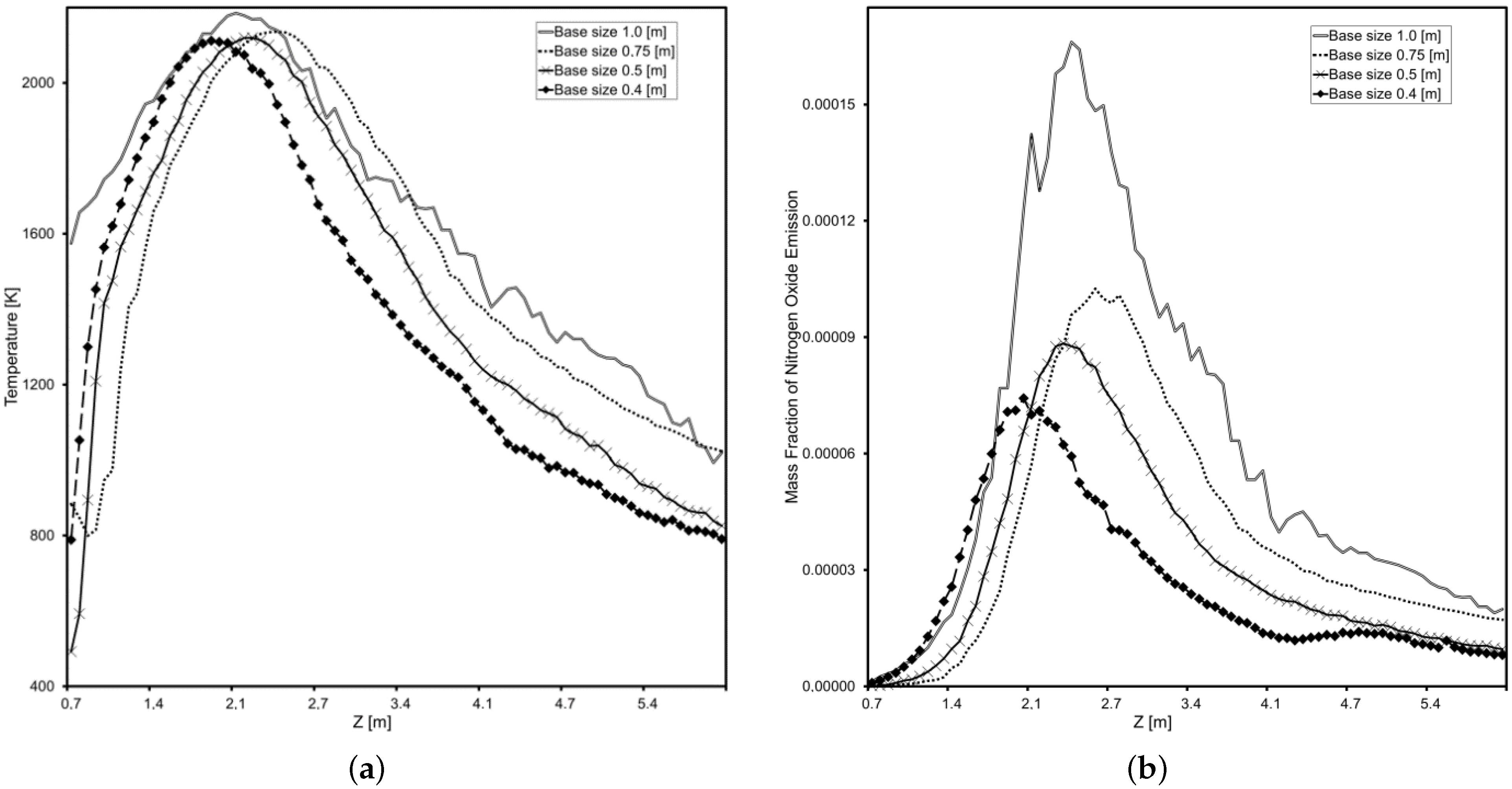
At the first stage, a study was carried out to select the required number of grid elements based on test calculations of the methane-air mixture. The simulated natural gas flow Q = 3936 nm${}^3$/h, which corresponds to 80% of the steam load of the E-500-13.8-560GMN (the other name TGME-464) type boiler. Figure 5 shows the results of a numerical calculation of the developed model at an air temperature at the burner inlet T = 477 K and an excess air coefficient $\alpha$ = 1.02.

As can be observed from Figure 5, as the base grid size increases, the calculation error increases. Additionally, it is necessary to pay attention to the machine resource spent when calculating on a computer, so for the “base” size of 0.5 m, more than 28 h of time were spent for 10 thousand iterations to calculate the combustion chamber with only one combined burner device. In this regard, for further calculations, we use a grid of the “basic” size of 0.5 m with the number of cells 2,787,464.

2.5. Choice of Combustion Model

At the second stage, a test study was carried out to select a model for a numerical experiment. The multidisciplinary STAR-CCM+ platform provides a wide range of such tools for modeling premixed methane-air mixtures.

As can be observed from Figure 6, with a change in the combustion model at the basic grid size determined in the previous step, the maximum temperature level remains at the same level, while the active combustion zone is shifting along the flame front of the simulated combustion chamber. At the same time, in each of the models, the condition for finding the maximum $N{O}_X$ content in the zone of maximum temperatures is observed. The choice of the Flamelet Generated Manifold (FGM) model is based on the possibility of using a pre-mixed flame.

2.6. Some of the Obtained Results of Forecasting Emissions of Harmful Substances

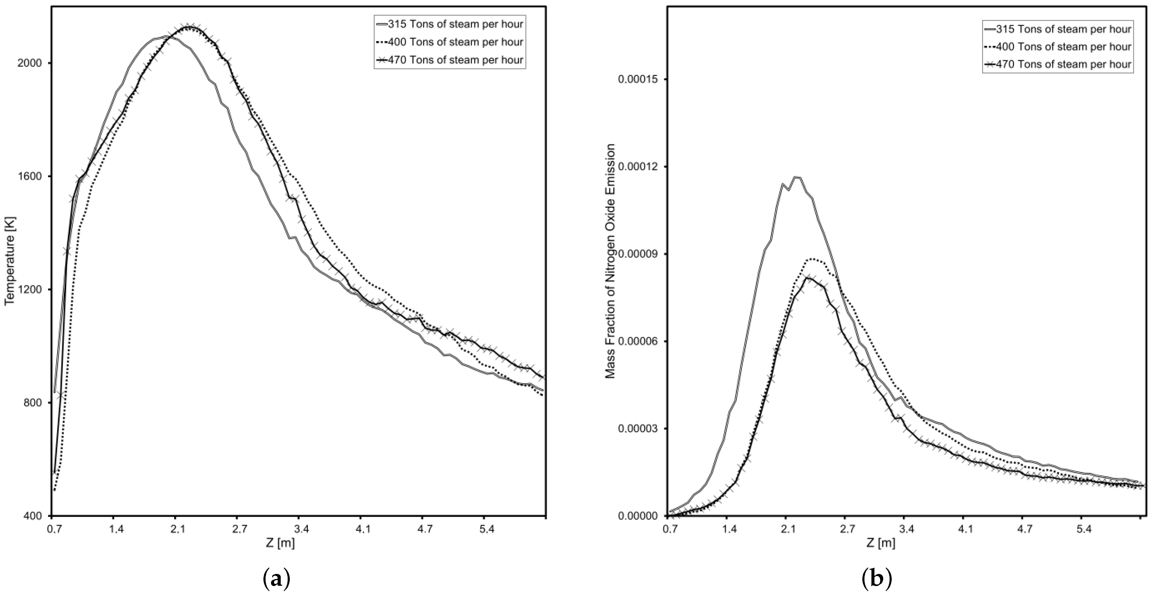
For the development of new technical and regime measures aimed at reducing C for the existing GMU-45 burner used in power boilers E-500-13.8-560GMN, it is important to have theoretical data for different steam loads. During computational experiments to study the emission of harmful substances, steam loads of 315 tons per hour (63%), 400 tons per hour (80%) and 470 tons per hour (94%) of the E-500-13.8-560GMN power boiler were simulated. Figure 7, shows the results of computational experiments with the excess air coefficient $\alpha$ = 1.06–1.03, and gas flow rate through one burner 2985–4550 m${}^3$/h. To obtain adequate results, the regime map of the operating power boiler E-500-13.8-560GMN was used as the initial data.

It can be observed from the figures that as the load increases, the temperature in the core of the flare and $C{O}_2$ increases, but at the same time, $N{O}_X$ emission turned out to be the maximum at a load of 315 tons per hour, which is explained by a large air excess factor.

In steam boilers of this type, one of the main methods for reducing $N{O}_X$ emissions is implemented–flue gas recirculation. The recirculation of combustion products into the combustion chamber leads to a decrease in the temperature of the torch and the alignment of the temperature fields in the furnace, which leads to an intensive suppression of the formation of thermal $N{O}_X$. There are several basic ways to supply recirculated gas to air ducts. The first method is the selection of flue gases in front of the regenerative air heater at temperatures above 300 °C and their introduction into the hot air box. In this case, the recirculating gases are transported by a special exhaust gas recirculation fan, which allows one to adjust the degree of recirculation gases supply within 0–25%, depending on the boiler load. The second method involves the selection of flue gases after the regenerative air heater at temperatures of 130–160 °C, and the cost of servicing the flue gas recirculation fan and its cost is less compared to the first method. Sometimes, due to the lack of free space for installing a flue gas recirculation smoke exhauster and additional gas ducts, a jumper is installed between the flue behind the smoke exhauster and the air duct in front of the blower fan. This recirculation method is the cheapest, but the degree of recirculation, as a rule, does not exceed 12–15% due to the additional load on the blower fan and smoke exhauster.

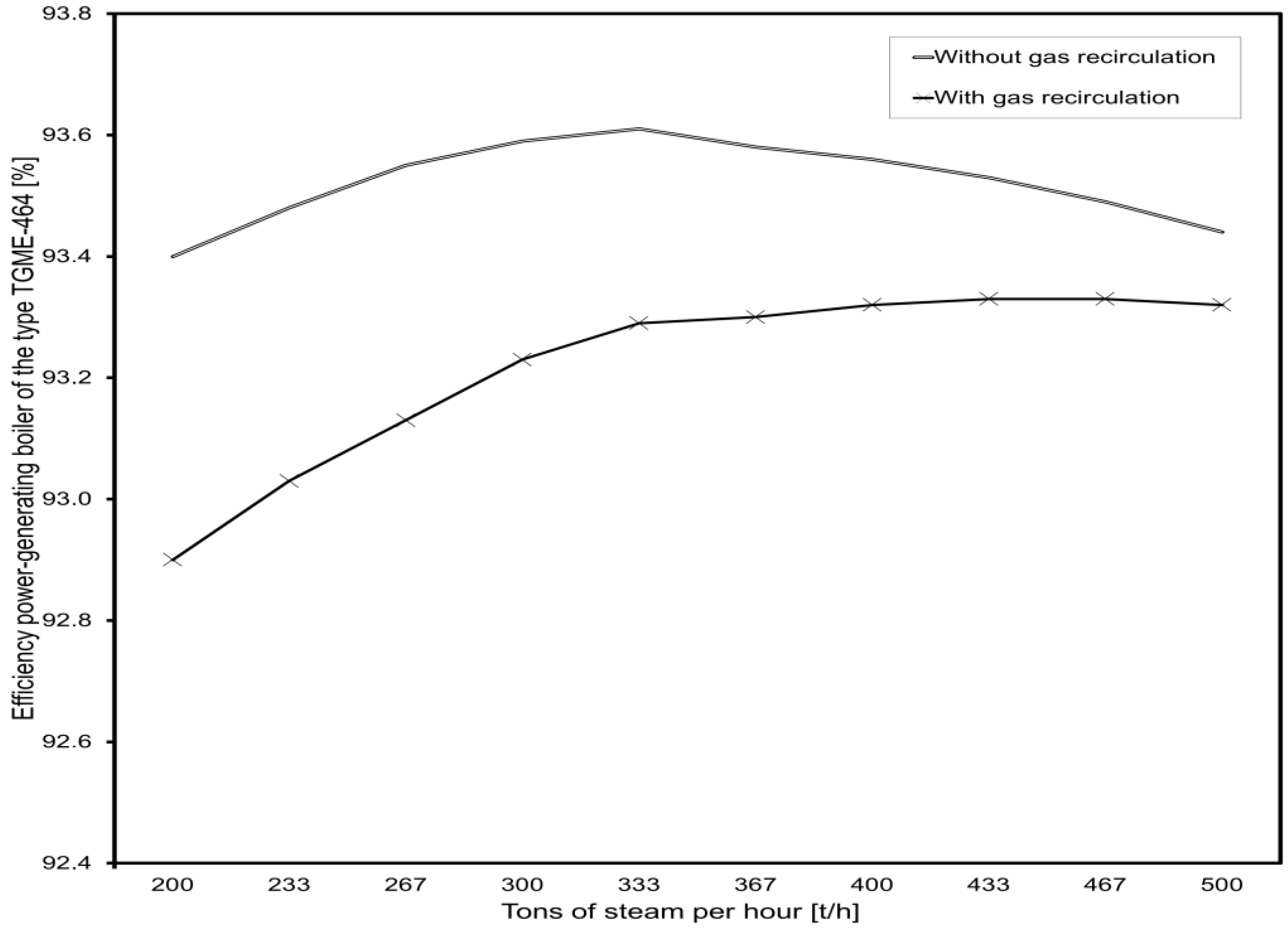
The limited use of flue gas recirculation is associated with a decrease in the economic performance of the boiler. The efficiency of the boiler is reduced by 0.01 ÷ 0.03% for every 1% of the degree of recirculation due to an increase in heat loss with flue gases due to an increase in flue gas temperature. Moreover, the consumption of electricity for the drive of the blower fan, the smoke exhauster and the flue gas recirculation smoke exhauster are growing. Figure 8 shows an example of a general reduction in the efficiency of a steam boiler from its load when implementing flue gas recirculation.

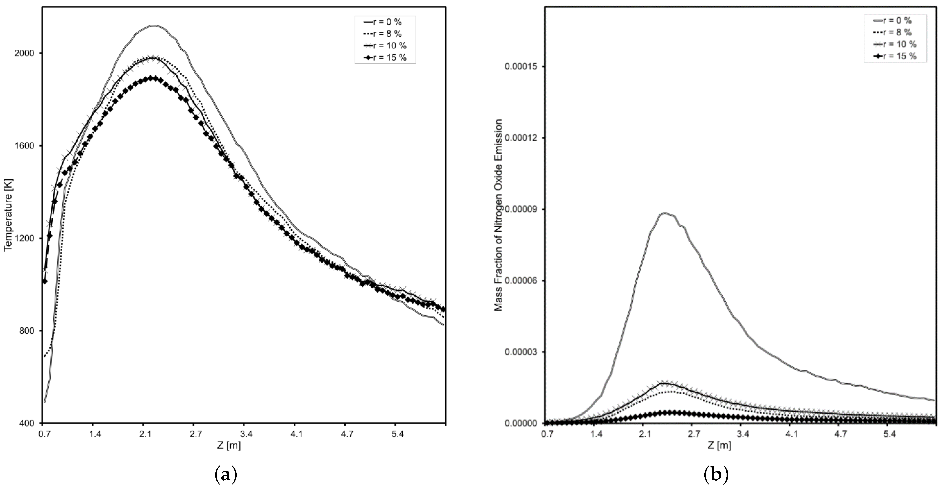
To organize the process of flue gas recirculation to reduce $N{O}_X$, it is important to have theoretical data on the change in the environmental performance of the boiler at different steam loads at different degrees of gas recirculation into the combustion zone. Figure 9 shows the results of a study of the emission of harmful substances from the E-500-13.8-560GMN power boiler at a steam load of 400 tons per hour. It is important to note the limited performance of E-500-13.8-560GMN blowers, due to which the maximum possible degree of recirculating gas supply decreases with increasing steam load.

From the analysis of Figure 9, with an increase in the degree of recirculation gas supply (r = 0 ÷ 15%), the $N{O}_X$ content decreases along the flame profile, which is explained by a decrease in the maximum temperature, which is the main indicator of the formation of thermal $N{O}_X$. The decrease in temperature in the zone of active combustion is explained by the increase in the volume of triatomic gases in the zone of natural gas combustion. At the same time, maximum efficiency is achieved at the maximum possible degree of recirculation gas supply (for this type of boiler, limited by the capacity of the blower fan). 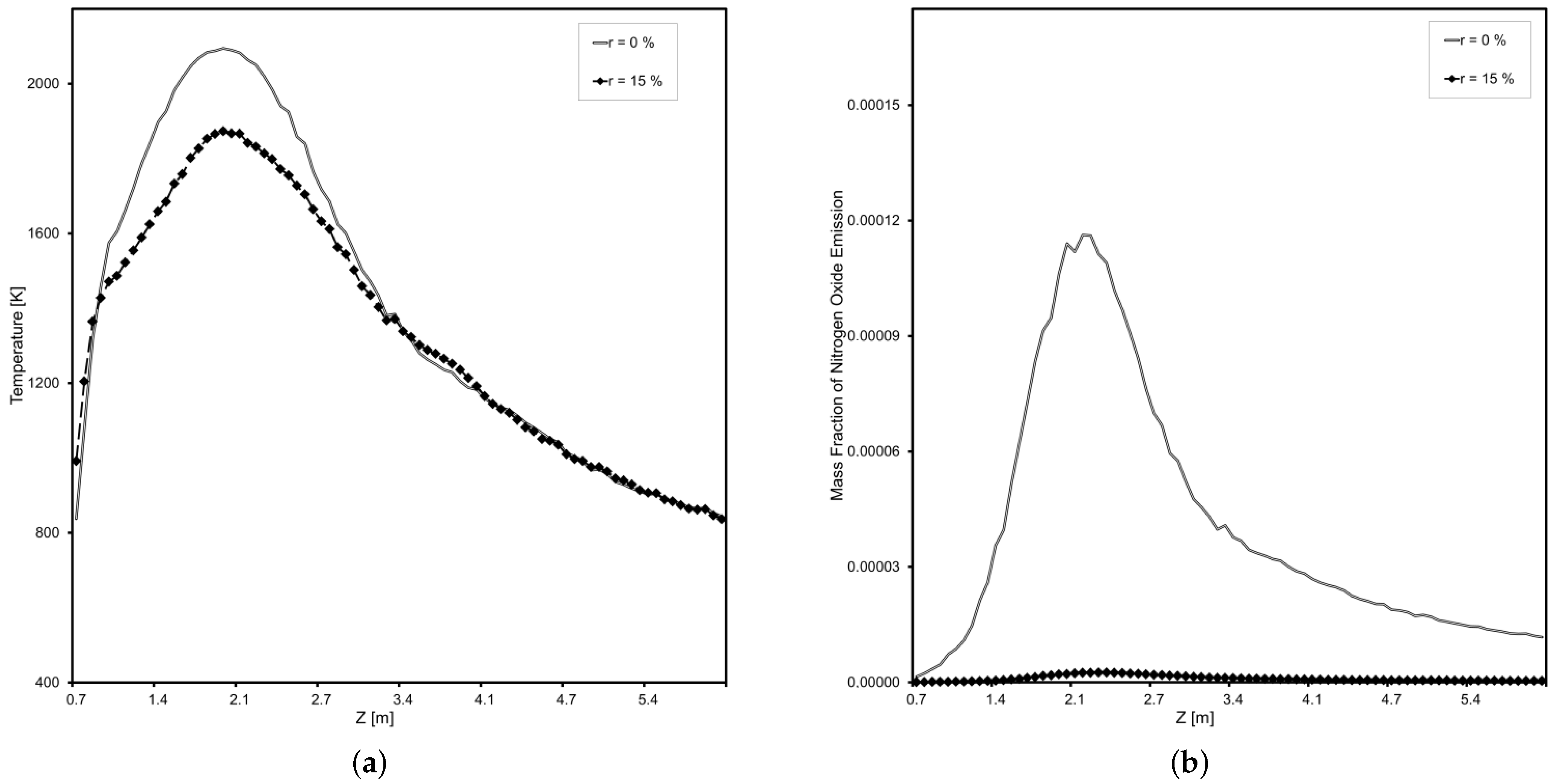Figure 10 shows the results of a study of the emission of harmful substances from the E-500-13.8-560GMN power boiler at a steam load of 315 tons per hour.

From the analysis of Figure 10, it can be observed that with the supply of 15% flue gas recirculation, the decrease in the maximum temperature in the core of the flare is up to 250 °C. A further increase in the efficiency of $N{O}_X$ emission suppression is possible by lowering the local temperature due to the reorganization of the degree of recirculation (without changing its total share) along the tiers of burners of power boilers, with most of them directed to the zone of maximum temperatures. The implementation of this technical solution can additionally neutralize one of the significant disadvantages of this method of reducing $N{O}_X$—reducing the efficiency of a power boiler: reorganization of the degree of recirculation allows, without loss of technology efficiency, to reduce the total share of flue gas recirculation, which will reduce heat losses with exhaust gases (due to flue gas temperature reduction) and the power expended on the drive of the blower fan and flue gas recirculation smoke exhauster [46].

3. Application of Machine Learning to Improve the Efficiency of Burners

3.1. Machine Learning Problem Statement

The influence of various indicators on the efficiency of burner devices (load, air flow, methane and biogas, fuel and oxidizer compositions, and others) is investigated. The efficiency of the burner is evaluated by the content of $N{O}_X$, $CO$, as well as by the temperature of the flue gases and the temperature in the core of the torch; in this case, three states of the device are assumed: optimal, satisfactory, and unsatisfactory.

There are known precedents in the form of the results of computational experiments to simulate the operation of the burner device: the values of the performance indicators and the corresponding performance characteristics.

This is a machine learning task: multiclass classification of the states of the burner device based on the results of the analysis of the received data (learning by precedents: “supervised”).

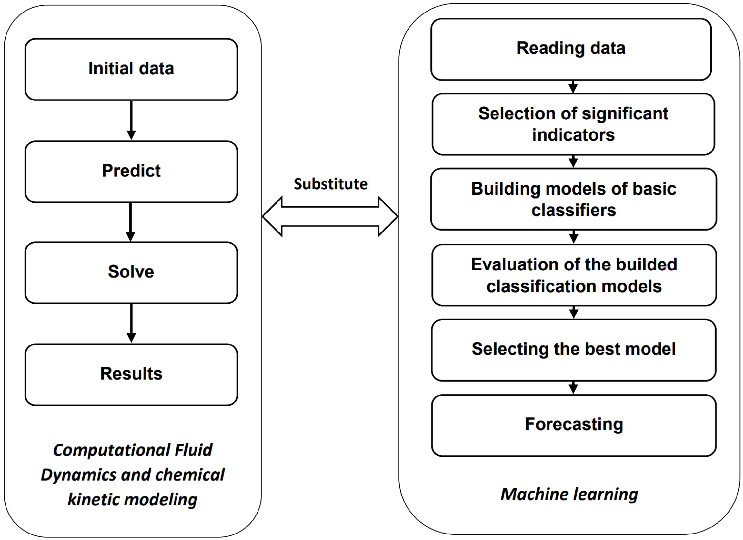
The purpose of this study is to develop a learning algorithm that provides the necessary accuracy of predicting the state of the device when setting new values of performance indicators (Figure 11).

3.2. Basic Machine Learning Methods

Many different methods can be used for multiclass classification. First, there are statistical methods of Fisher’s discriminant analysis. Many other algorithms are also based on the methods of probability theory and mathematical statistics. These are the naive Bayes classifier, logistic regression, support vector machines, nearest neighbor methods and others. Decision trees are often used in classification problems.

Of the intelligent methods, the main one is the method of artificial neural networks: the best results are obtained using deep learning, but a large amount of initial data is required: tens of thousands of observations or more. Since it seems unrealistic to obtain such a volume of data in the problem under consideration, this method is not used.

All these methods are described in detail in the literature [47,48,49,50,51].

A special group consists of compositional methods, which represent an ensemble of individual algorithms. The two main compositional methods–bagging and boosting–give higher accuracy on a specific data set compared to separate algorithms. Compositional methods use the same classification method, built either on different subsets of the sample, or compensating for the errors of the previous iteration at each step.

Let us consider in more detail one of the variants of compositional methods, which turned out to be the best in the problem under consideration—“random forest”. Random forest is a machine learning algorithm proposed by L. Breiman [51]; it uses an ensemble (committee) of decision trees. The algorithm combines bagging (random selection with return) and the random subspace method. It consists of many independent decision trees, using a random sample of observations from the training set and a random set of metrics to make node split decisions. The random forest is used to solve problems of classification, regression and clustering.

The classification of objects is carried out by voting: each tree of the committee assigns the object being classified to one of the classes, and the one with the most trees wins. The optimal number of trees is selected in such a way as to minimize the classifier error on the test sample.

The method has high prediction accuracy, is insensitive to monotonic transformations of indicator values, rarely retrains: adding trees almost always only improves the composition, but after reaching a certain number of trees, the learning curve reaches an asymptote. The disadvantages include the fact that, unlike a single tree, the results of random forests are harder to interpret; in addition, it is difficult to save the result due to the too large memory size of the final models.

Exactly this method turned out to be the best in solving the problem of estimating the efficiency of burners.

When using the aggregated approach [52,53,54], various classification methods based on the training set are used together. To achieve the best result, a full enumeration of sets from all basic methods can be applied. However, studies have demonstrated that the use of more than two basic classifiers in the aggregate does not provide a significant increase in accuracy. At the same time, the aggregation method (by the mean, by the median, or by voting) also does not have a significant impact on the quality of the classification. In this regard, the aggregation of two classifiers by the average value was used.

For example, for the support vector machine, the probability that the state of the object belongs to the k-th class is:

$$P\left(Y=k|X\right)=\frac{{\displaystyle exp\left(\sum _{j=1}^p{w}_{kj}{x}_j+w_{k,o}\right)}}{{\displaystyle \sum _{i=1}^m\left(\sum _{j=1}^p{w}_{ij}{x}_j+w_{i,o}\right)}}$$

(21)

where $w_{ij}$—support vector machine parameters determined using the Lagrange multiplier method for each of the m classes.

For boosting methods, this probability is defined as:

$$P\left(Y=k|X\right)=\frac{{\displaystyle exp\left(\sum _{t=1}^T{\alpha }_{kt}{h}_t\right)}}{{\displaystyle \sum _{i=1}^m\left(\sum _{j=1}^T{\alpha }_{it}{h}_t\right)}}$$

(22)

where $h_t\left(x\right)$—basic boosting classifiers; T—number of base classifiers, ${\alpha }_{it}$—weighted voting coefficient for the corresponding classifier $h_t\left(x\right)$. The mathematical model of the aggregated mean value classification method for two basic methods—support vectors and boosting–will take the form:

$$\widehat{P}\left(Y=k|X\right)=\frac{1}{2}\left[\frac{{\displaystyle exp\left(\sum _{j=1}^p{w}_{kj}{x}_j+w_{k,o}\right)}}{{\displaystyle \sum _{i=1}^m\left(\sum _{j=1}^p{w}_{ij}{x}_j+w_{i,o}\right)}}+\frac{{\displaystyle exp\left(\sum _{t=1}^T{\alpha }_{kt}{h}_t\right)}}{{\displaystyle \sum _{i=1}^m\left(\sum _{j=1}^T{\alpha }_{it}{h}_t\right)}}\right]$$

(23)

The expediency of using aggregated classifiers is such that when conducting a binary classification, this approach led to a significant increase in the quality of training [52]. In a number of cases, aggregation according to Formula (23) led to an increase in the value of the F-measure when solving the problem of estimating the efficiency of burners.

3.3. Criteria for the Quality of Education

To assess the quality of machine learning, three different criteria are most often used: the average error on the test sample (or vice versa, the proportion of correct answers), AUC—area under ROC curve—the area under the ROC curve (error curve) and F-measure.

The F-score is calculated based on two metrics, precision and recall. The precision is the percentage of correctly identified objects of one class among all objects assigned by the system to this class. The recall is the percentage of correctly identified objects of one class among all objects of this class in the test sample.

$$P=\frac{TP}{TP+FP};$$

(24)

$$R=\frac{TP}{TP+FN},$$

(25)

where $TP$ (true-positive) is the number of true-positive decisions (for example, the number of objects of the 1st class assigned to the 1st class), $FP$ (false-positive) is a false positive decision (for example, the number of objects of the 2nd class, assigned to the 1st class), $FN$ (false-negative)—a false negative decision (the number of objects of the 1st class assigned to the 2nd class). The F-measure is determined by the formula:

$$\mathrm{F}=\frac{2PR}{P+R},$$

(26)

it is the harmonic mean between precision and recall. Such a measure is the most informative quality indicator for unbalanced classes: the closer the F value is to one, the higher the classification quality.

A useful quality characteristic of a multiclass classification is the confusion matrix. The confusion matrix is an m*m matrix, where m is the number of classes. The matrix shows how many examples from each class were identified correctly (diagonal values) and how many observations from each class were incorrectly identified as the kth class (k = 1, …, m). Each row of the matrix represents instances in the predicted class, and each column represents instances in the actual class. The sum of all off-diagonal values of the matrix shows the number of errors made by the classifier.

3.4. Burner Performance Indicators Obtained from the Results of a Computational Experiment

Based on the results of a series of 309 computational experiments, using the complex of models presented in Section 2, 20 factors that affect the efficiency of the burner device were identified (

Table 1. Indicators affecting the efficiency of the burner.

Symbol	Name	Unit of Measure	Minimum	Maximum
$X_1$	Steam load	tons/h	170	500
$X_2$	Air consumption	m${}^3$/h	4847	61,152
$X_3$	Methane consumption	m${}^3$/h	0	5375
$X_4$	Biogas consumption	m${}^3$/h	0	5000
$X_5$	$C{H}_4$	%	30.41	98
$X_6$	$C_2{H}_6$	%	0	14.58
$X_7$	$C_3{H}_8$	%	0	9.09
$X_8$	$C{O}_2$	%	0	31.75
$X_9$	$N_2$	%	0	1.05
$X_{10}$	$H_{2}S$	%	0	0.11
$X_{11}$	$H_2$,	%	0	50.1
$X_{12}$	$O_2$	%	0.179	0.232
$X_{13}$	$N_2$	%	0.750	0.768
$X_{14}$	$C{O}_2$	%	0	0.023
$X_{15}$	$H_{2}O$	%	0	0.048
$X_{16}$	Inlet air temperature	K	446	533
$X_{17}$	Fuel temperature	K	10	25
$X_{18}$	Swirler blade angle	degrees	0	50
$X_{19}$	Grid size	m	0.1	1
$X_{20}$	Excess air ratio		0.88	1.5

).

The efficiency of the burner is evaluated by the following indicators: $N{O}_X$ content ($Y_1$), $CO$ content ($Y_2$), flue gas temperature ($Y_3$) and flame core temperature ($Y_4$); in this case, three possible states of the device are assumed: optimal (class 1), satisfactory (class 2) and unsatisfactory (class 3).

The optimal state of the burner is considered when $Y_1$ < 125, $Y_2$ < 100, $Y_3$ = 343–381, $Y_4$ = 1600–1700; satisfactory—with $Y_1$ = 125–290, $Y_2$ = 100–300, $Y_3$ = 381–393, $Y_4$ = 1700–2100; unsatisfactory—with $Y_1$ > 290, $Y_2$ > 300, $Y_3$ > 393, $Y_4$ > 2100.

Taking into account these ratios, it was found that out of 309 observations, 31 (10%) belong to class 1, 164 (53%) belong to class 2 and 114 (37%) belong to class 3. There is a significant imbalance in the data: observations belonging to class 1 are much less than to classes 2 or 3. This means that in practical calculations, the F-measure will be the main criterion for the quality of machine learning.

4. Results and Discussion of a Computational Experiment

The presence of correlations between indicators was investigated. The correlation matrix showed a linear relationship between the pairs of indicators $X_7$ ($C_3{H}_8$) and $X_{1}1$ ($H_2$), as well as between $X_8$ ($C{O}_2$) and $X_{10}$ ($H_{2}S$). When conducting machine learning, the $X_{10}$ and $X_{11}$ indicators were excluded from the feature matrix. A strong correlation (sample correlation coefficient r > 0.9) takes place between the pairs of indicators $X_4$–$X_5$, $X_4$–$X_9$, $X_5$–$X_9$, $X_6$–$X_7$, $X_6$–$X_{11}$. At the same time, a weak but significant (according to the Student’s t-test) correlation of indicators with class numbers (r < 0.4) was found. 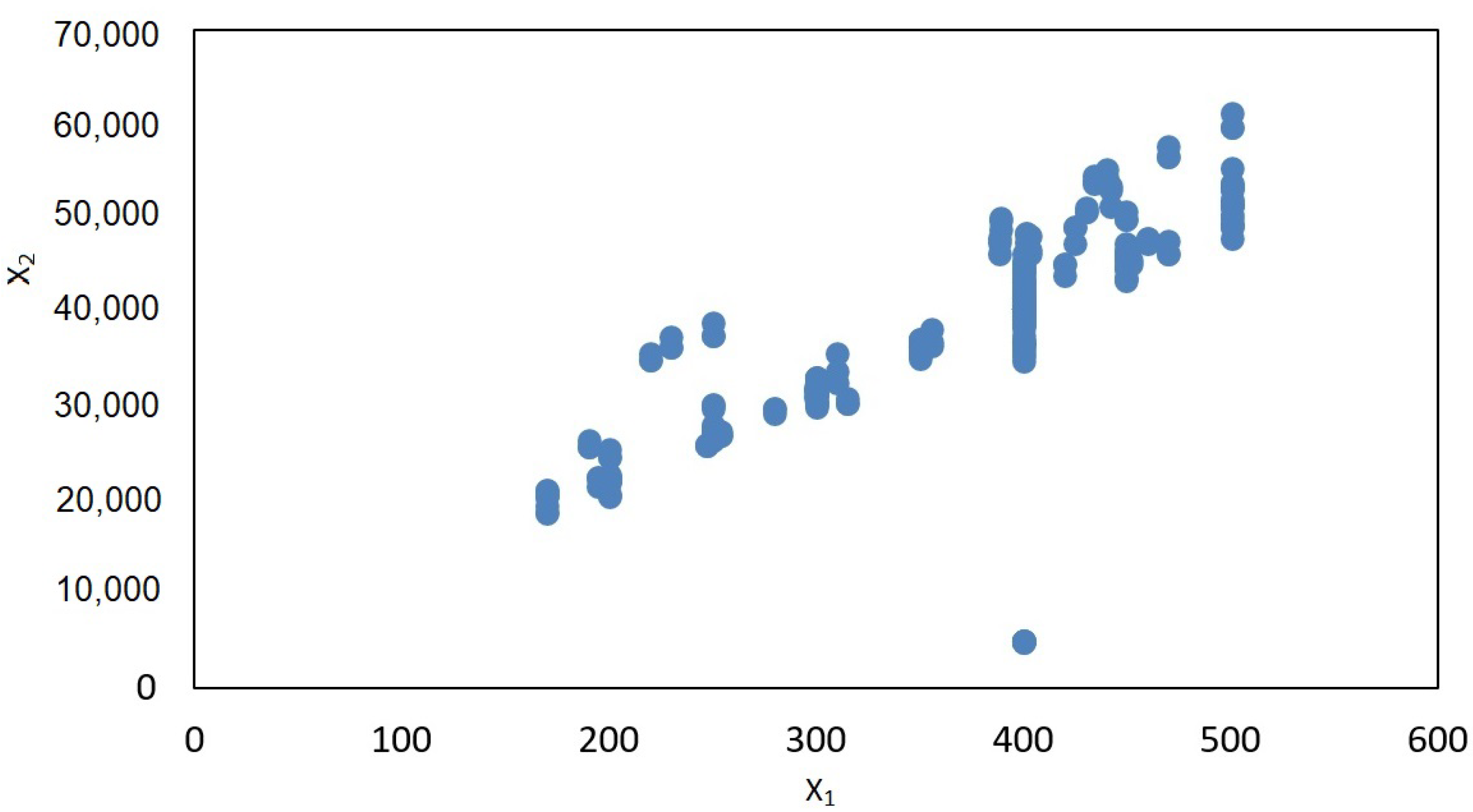For example, for the $X_1$ indicator, the correlation coefficient is r = 0.34; for the indicator $X_{19}-r$ = 0.36. The presence of outliers in the data was estimated from scatterplots between pairs of indicators. Figure 12 shows the outlier at the point with coordinates (400; 4896). The corresponding rows of the feature matrix and the response vector ($x_i$, $y_i$) were removed from the sample: a total of nine outliers were found.

To build a multiclass classification, a special program was developed in the Python programming language. It used the Sklearn library (scikit-learn) from which constructors for classification algorithms are imported: LogisticRegression, LinearDiscriminantAnalysis, KNeighborsClassifier, DecisionTreeClassifier, GaussianNB, SVC—support vector machine, RandomForestClassifier and AdaBoostClassifier. Moreover, ready-made modules for calculating multiclass classification metrics are imported from the Sklearn library.

The mean aggregation method was programmed by hand but using a Python function to find the probabilities that each object belongs to the corresponding class: predict_proba.

The program provides input of the initial data file, splitting it in each ratio into training and test parts in a random way, conducting cross-validation with a user-specified number of blocks.

The result of the program is the calculation of three measures of classification quality for the test sample (the proportion of correct answers, F-measures, and confusion matrices) for basic, combined, and aggregated classifiers. The user, depending on the nature of the initial data, selects the best criterion, which is used to predict the state of the object. According to the newly set (found) indicators of the functioning of the object, it is predicted to which class its state belongs.

When starting the program, the initial data file is first requested (we have a table of 300 rows and 19 columns, of which 18 are indicators, the 19th column is the class to which the corresponding row belongs), then the volume of the test sample in percent (we take initially K = 20) and the number of cross-validation blocks (assuming N = 4). The division of the initial data into training and test parts is conducted randomly. The program displays the percentage of correct answers and the value of the F-measure on the test set for various algorithms, as well as the confusion matrix for the best classifier.

Comparison of the effectiveness of various methods for solving the tasks set is presented in

Table 2. Percentage of correct answers on the test set for various basic machine learning methods.

Method	Percentage of Correct Answers, %
Logistic regression	73.33%
Discriminant Function Analysis	71.67%
K-Nearest Neighbors Algorithm	80.00%
Support vector machine	56.67%
Naive Bayes classifier	21.67%
Decision tree	90.00%
Random forest	91.67%
AdaBoost	70.00%

,

Table 3. F-measure values on a test set under various basic machine learning methods.

Method	F-Measure
Logistic regression	0.713
Discriminant Function Analysis	0.700
K-Nearest Neighbors Algorithm	0.802
Support vector machine	0.490
Naive Bayes classifier	0.206
Decision tree	0.898
Random forest	0.916
AdaBoost	0.691

and

Table 4. F-measure values on the test sample with different aggregation methods.

Method	F-Measure
Random forest + Support vector machine	0.898
Random forest + K-Nearest Neighbors Algorithm	0.882
Random forest + AdaBoost	0.882
Random forest + Logistic regression	0.866
Support vector machine + K-Nearest Neighbors Algorithm	0.830
Support vector machine + AdaBoost	0.844
Support vector machine + Logistic regression	0.640
Support vector machine + Discriminant Function Analysis	0.710
K-Nearest Neighbors Algorithm + AdaBoost	0.867
K-Nearest Neighbors Algorithm + Logistic regression	0.799
K-Nearest Neighbors Algorithm + Discriminant Function Analysis	0.758
AdaBoost + Logistic regression	0.867
AdaBoost + Discriminant Function Analysis	0.805
Logistic regression + Discriminant Function Analysis	0.713

.

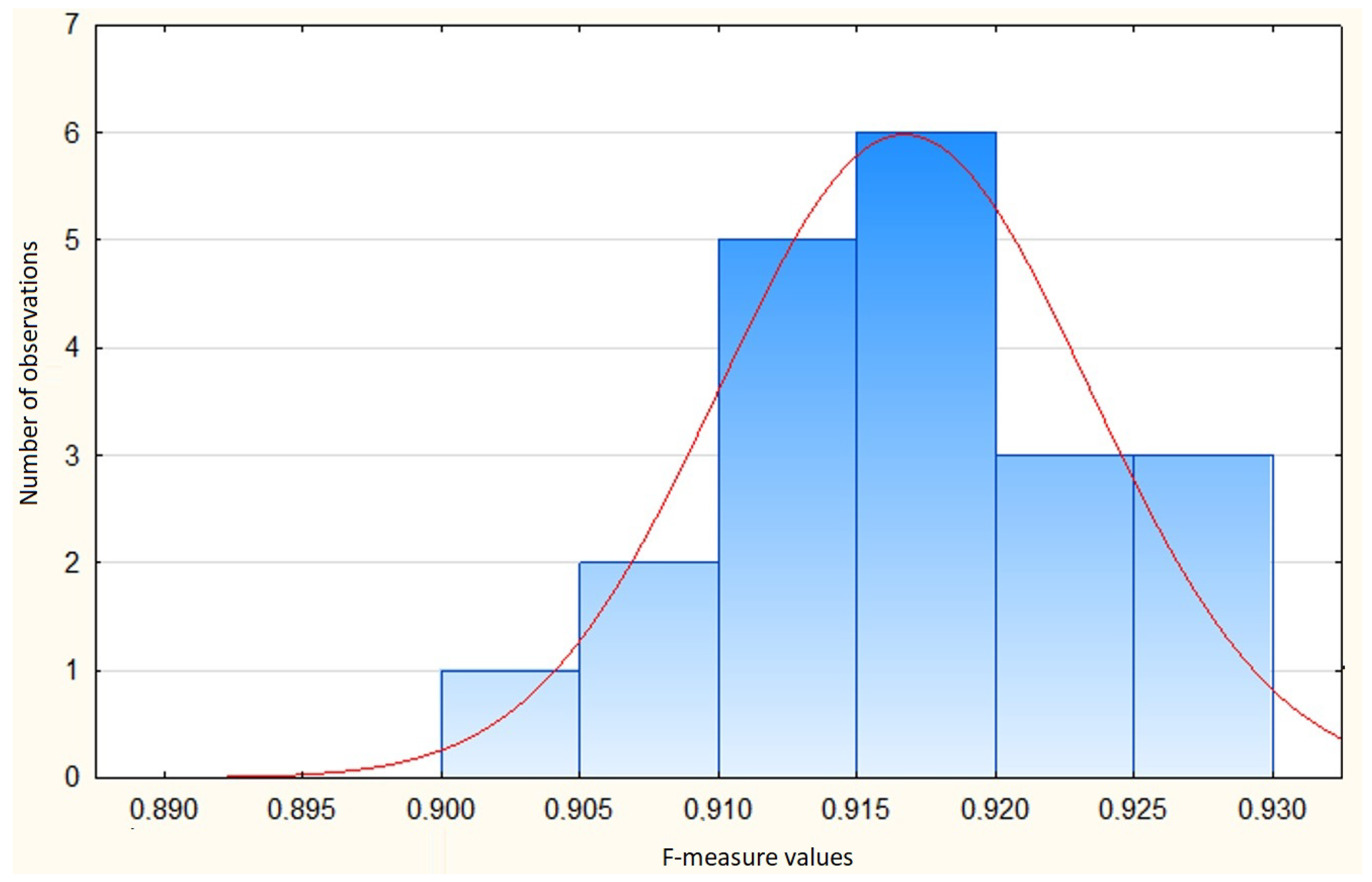
In the above example, the best classifier was a random forest with F-measure of 0.916. The confusion matrix shows that the algorithm correctly assigned six observations out of sixty contained in the test sample (20% of 300) to the first class, while there are no errors. Thirty observations were assigned to the second class (with two observations of the second class mistakenly taken for the third class). Nineteen observations were correctly assigned to the third class, in three cases the algorithm made a mistake: observations of the third class were assigned to the second.

Since the formation of the test sample is conducted randomly, the results will be slightly different each time the program is run. It is of interest to estimate the dispersion of the F-measure values. For this purpose, the sample was launched several times. The result is shown in Figure 13, where a distribution histogram is shown using the Statistica system with a normal distribution curve plotted on it. The Shapiro-Wilk test for testing the normality hypothesis for small samples confirms the normality of the distribution of the F-measure. The mean value turned out to be 0.9167, standard deviation 0.0067. The 95 confidence interval of the F-measure was (0.914; 0.920).

When assessing the impact of the test sample share on the quality of education, the values of the percentage of this sample were entered from 10% to 30% with a step of 5%. The test results are presented in

Table 5. F-measure value for different test sample sizes.

Share of the Test Sample	10%	15%	20%	25%	30%
F-measure value	0.901	0.910	0.917	0.881	0.900

.

It can be seen that the proportion of the test sample has an ambiguous effect on the value of the F-measure. At the same time, a change in this proportion can increase or decrease the value of the measure by several percent (in the tests carried out, up to 4%). When testing burner devices, the best option turned out to be the one in which the test sample is 20% of all initial data. Note that in all tests, the random forest turned out to be the best algorithm.

It is also of interest to assess the impact of the number of cross-validation blocks on the quality of training.

Table 6. F-measure value for different number of cross-validation blocks.

Number of Blocks	4	5	6	10
F-measure value	0.915	0.899	0.878	0.883

shows the results of the corresponding tests with a test sample of 20%.

The discrepancy in the values of the F-measure was about 4%. The results for classification using a random forest are given, although, unlike the previous experience, where the random forest turned out to be the best algorithm in all tests, here, with N = 6, the aggregate classifier turned out to be the best, including the support vector machine and boosting (AdaBoost), for which F = 0.903.

So, the best values of the studied parameters turned out to be the size of the test sample K = 20%) and the number of cross-validation blocks N = 4. The developed program allows predicting the state of the burner device using the resulting classifier. We enter new values of eighteen indicators, and as a result, we get a predicted state (class) at the output.

Figure 14 shows the ranking of indicators by significance (the Statistica system was used), which allows, with a large number of them, to reduce the least significant indicators.

As follows from Figure 14, in our study, the most significant indicators were $X_{14}$ ($C{O}_2$, its significance is taken as 1), $X_1$ (load, its significance is 0.99) and $X_2$ (air consumption, its significance is 0.93), the least significant—$X_{10}$ ($H_{2}S$, its significance is 0.18).

5. Conclusions

The paper proposes a mathematical model of a non-stationary turbulent combustion process, which takes into account the swirl of the flow. As a result of the performed mathematical modeling and numerical study of a non-stationary turbulent gas flow with flue gas recirculation on the STAR-CCM+ multidisplinary platform, it was found that the greatest reduction in emissions is achieved at a recirculation degree of 15%, and a variant of further reduction of the local temperature, which is the main indicator of the formation of thermal $N{O}_X$, was also proposed.

Based on the data obtained, several different machine learning methods were tested to classify the state of the burners in order to select the best one. The aggregation of machine learning methods was performed—in binary classification problems, this approach showed a significant increase in the quality of training. A study of the influence of various factors on the quality of education was carried out (similar studies were carried out earlier, but for burners it is carried out for the first time).