Harris Hawk Optimization-Based Deep Neural Networks Architecture for Optimal Bidding in the Electricity Market

Abstract

In the power sector, competitive strategic bidding optimization has become a major challenge. Digital plate-form provides a superior technical base as well as backing for the optimization’s execution. The state-of-the-art frameworks used for simulating strategic bidding decisions in deregulated electricity markets (EM’s) in this article are bi-level optimization and neural networks. In this research, we provide HHO-NN (Harris Hawk Optimization-Neural network), a novel algorithm based on Harris Hawk Optimization (HHO) that is capable of fast convergence when compared to previous evolutionary algorithms for automatically searching for meaningful multilayered perceptron neural networks (MPNNs) topologies for optimal bidding. This technique usually demands a considerable amount of time and computer resources. This method sets up the problem in multi-dimensional continuous state-action spaces, allowing market players to get precise information on the effect of their bidding judgments on the market clearing results, as well as implement more valuable bidding decisions by utilizing a whole action domain and accounting for non-convex operating principles. Due to the use of the MPNN, case studies show that the suggested methodology delivers a much larger profit than other state-of-the-art methods and has a better computational performance than the benchmark HHO technique.

1. Introduction

Many economic systems used in the power sector’s research are centralized, optimize the objective of the system (e.g., maximizing social welfare) and assume that market participants behave in a perfectly competitive (price-taking) manner. However, increasing attempts to deregulate the power industry have resulted in increased competition among several self-interested (profit-driven) market competitors, particularly in the production and supplier domains. Due to the fact that self-interested market player’s nature is not always allied with global targets, existing centralized frameworks are no longer able to give accurate perspectives. Consequently, emerging market methods that are useful are capable of tracking the strategic (price-making) behavior of self-interested market players as well as recognizing the market outcomes that result from their interactions [1].

Power production and transmission have evolved from vertically integrated operations to market-driven operations in the world’s main economies. The liberalization of the power sector has resulted in increased effectiveness through rivalry among market players. In the energy sector, generators are the ideal candidates for iteration in rivalry to enhance the effectiveness and competitiveness in allocation of resources, as well as to compete for the cheapest cost with the superior products. Real-time balancing and day ahead are the two kinds of energy markets. In a real market, rivals purchase energy during the business days, and energy prices are established daily or hourly based on requirement and production. A study of spikes in electricity price has been conducted in reference [2]. In a day ahead market, participants purchase wholesale energy in the day-ahead power sector a day before the operating days, and the discrepancy among planned and real needs on the operating day is compensated in the real time marketplace [3].

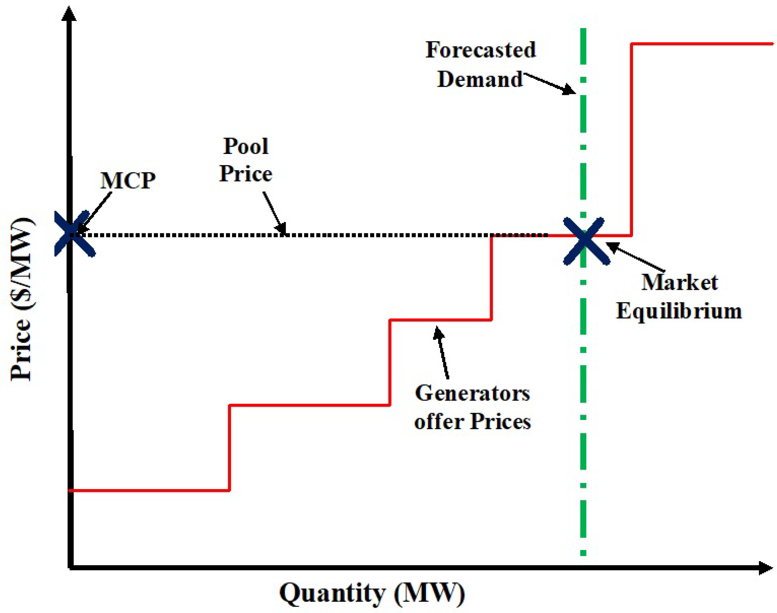
An energy pool in the day ahead marketplace is one of the key services in the wholesale competitive liberated energy sector in the reformation of the electrical energy industry across the world [4]. The Independent System Operator (ISO) finalized generators bids for every hour of the next day in the day ahead marketplace. So each generator provides bids to the ISO for each hour of the following day. The proposed price must be greater than zero but less than the industry restriction. The ISO examines bids to establish the hourly MCP and the amount of power to be delivered by each generator’s framework of the proposed cost and MCP [5]. The EM mechanism that is explained above is shown in Figure 1.

A two-auction system exists: (a) uniform price, which provides just at agreed level (with such a price available at a cheaper clearance cost) based on hourly MCP, and (b) pay-as-bid auction, which pays at the accepted level of each generator based on its applicable rate [6]. In every marketplace, the price-forecasting process is linked to: (a) size of the market (the amount of prospective producers and consumers); (b) market structure and process (including such payment methods or accessibility) [7]; (c) degree of access to market and player’s information; and (d) risk analysis options [8]. Even so, there really are discrepancies among energy and other commodity markets, such as:

a

Energy cannot be conveniently collected and should be used instantaneously produced because the physiological delivery method works much quicker than any industry [9];

b

Energy transportation needs to carry massive losses and expenses, as well as special distribution facilities;

c

Power systems are the most destructive especially in comparison to other traded commodities, and all of these factors conspire to create energy as the most turbulent commodity.

d

Although production and consumption should be coordinated at all times, electricity supply must be demanded precisely at any given time from across the system.

e

At the annual, weekly, and daily levels, the MCP demonstrates considerable periodicity [10].

f

The electrical consumer has no control over which generator creates the load, and the generator has no control over which customers receive electricity [10].

Optimization approaches influenced by nature: swarm intelligence is a popular branch of artificial intelligence in which algorithms are created by emulating the intelligent behaviour of various animals such as wolves, whales, ants, lions, crows, and bees. HHO [11] is a swarm intelligence-based method that was recently discovered to solve real-world optimization problems. Ali Asghar Heidari et al. found it in 2019 [11] after being inspired by Harris ‘hawks’ cooperative behaviour and chasing style in a setting known as amazement jump. A few hawks agreeably jump a victim from varied angles in order to astonish it. Harris hawks can find a variety of pursuing examples based on the rabbit’s distinct concept of situations and getting away from instances. To nurture an optimization method, this research endeavour numerically simulates such powerful examples and behaviours. Regardless of the fact that there are various nature-inspired optimization methods based on stochastic behaviour available in the literature, the HHO algorithm was chosen in this study due to its acceptable search space exploration strength when compared to other meta-heuristic algorithms. A multi-strategy search was inspired by the prey hunting behaviour of Harris’s hawk. The least squares support vector machine (LSSVM) was utilised to represent the reactive power output of the synchronous condenser, and the developed Harris Hawks optimization algorithm was employed to optimise it.

Times series system [12], GARCH system [13], a mixture of wavelet transform and ARIMA [14], fuzzy auto regression framework [15], game theory [16], Bayesian optimization [17], neural network [18], and a combination of a machine learning algorithm and bat [19] have all been presented in the literature as methodologies for predicting electricity prices. Game theory, time series models, and simulation models make up the MCP prediction method; time series architectures are classified into three categories: stochastic models, machine intelligence models, and casual models [20].

1.1. Related Work

ANN has been identified to be the most appropriate model for predicting MCP from the above described models. They can evaluate the complicated relationship among next day MCP and past information of demand and other factors such as type of day, load, temperature, settling point, period, and so on. Among the most extensively utilized techniques for forecasting MCP judging by past data are NN architectures [21]. Authors used an NN to estimate MCP for the Australian power industry for many hours. Because the synthetic data and the Euclidean distance norm with normalized considerations were used to pick comparable days, the study revealed a significant exponential relationship with a rise in the hourly price prediction from 9.75% for one-hour-ahead forecasts to 20.03% for six-hour-ahead forecasts [22].

A Combinatorial Neural Network (CNN) was presented by Abedinia et al. to predict MCP in the Pennsylvania-New Jersey-Maryland (PJM) and mainland Spain markets. The parameters of the NN in CNN are optimized using the Chemical Reaction Optimization (CRO) technique in this system, and the mean WME is equivalent to 4.04% [5]. Authors created a novel hybrid method for predicting MCP in the Spanish and Pennsylvania-New Jersey-Maryland energy markets by merging the bat optimization with an NN; numerical results reveal that the average MAPE value is less than 1% [19]. Anbazhagan and Kumarappan suggested a model to predict MCP in the Spanish and New York electrical markets, with improvements in the average MPCE of 0.7 percent and 0.9 percent above the NN method, correspondingly [23].

The above-mentioned NN methods can be subdivided as: a heuristic technique whihc was used to measure the periodicity pattern of MCP in group 1, and another which was used to improve NN performance in group 2. Each of these qualities has indeed been addressed in this article. It is difficult to enhance MCP forecast accuracy because of its inherent stochastic and nonlinear tendencies. As a result, we report a novel hybrid model architecture that combines NN, PSO, and GA algorithms. Rather than using the classic back propagation method, PSO is used to enhance the learning power of a conventional neural network and optimize the weights of the NN, resulting in a local optimal configuration [19]. The GA is used to optimize the number of hidden layers on the NN [19] because networks are important to a number of neurons in their hidden layers. Since MCP has a periodicity tendency, the K-means method was used to analyse the NN’s training dataset and identify MCP’s periodicity trend [24]. This study proposes a machine learning-driven portfolio optimization methodology for virtual bidding in electricity markets that takes both risk and price sensitivity into account. To maximise profit, an algorithmic trading strategy is built from the standpoint of a proprietary trading firm [25]. The goal of this article is to maximise power market transactions and clearing price using metaheuristic algorithms. To achieve feasible results in a short amount of time, the exhaustive search algorithm is implemented using a parallel computer architecture. The global optimal outcome is used as a metric to compare the effectiveness of various metaheuristic algorithms. The results, discussion, comparison, and recommendations for the suggested set of algorithms and performance tests are presented in this work [26]. This article gives a case study of Pakistan’s electricity system, with information on electricity generated, connected load, frequency deviation, and load shedding during the course of a 24-h period. The data were evaluated using two methods: a traditional artificial neural network (ANN) with a feed forward back propagation model and a Bootstrap aggregating or bagging approach.

1.2. Major Contributions and Paper Structure

As previously stated, the following is a summary of our suggested method’s contribution:

a

The article presents a novel fusion architecture for optimal bidding in the power industry that fuses neural networks, and HHO.

b

In order to select the best records from past data to acquire NN, hourly data have been clustered based on the demands and bidding data of market participants;

c

To check the efficacy of HHO-NN, the results are compared against some recently developed, strong algorithms.

The arrangement of this manuscript is systematized as follows in Figure 2.

2. Problem Formulation

The following section presents a brief overview of the Gen-Co bidding strategy approach as well as the issue’s algebraic formulation. The sub-sections that follow cover everything that was previously mentioned.

2.1. Bidding Strategy

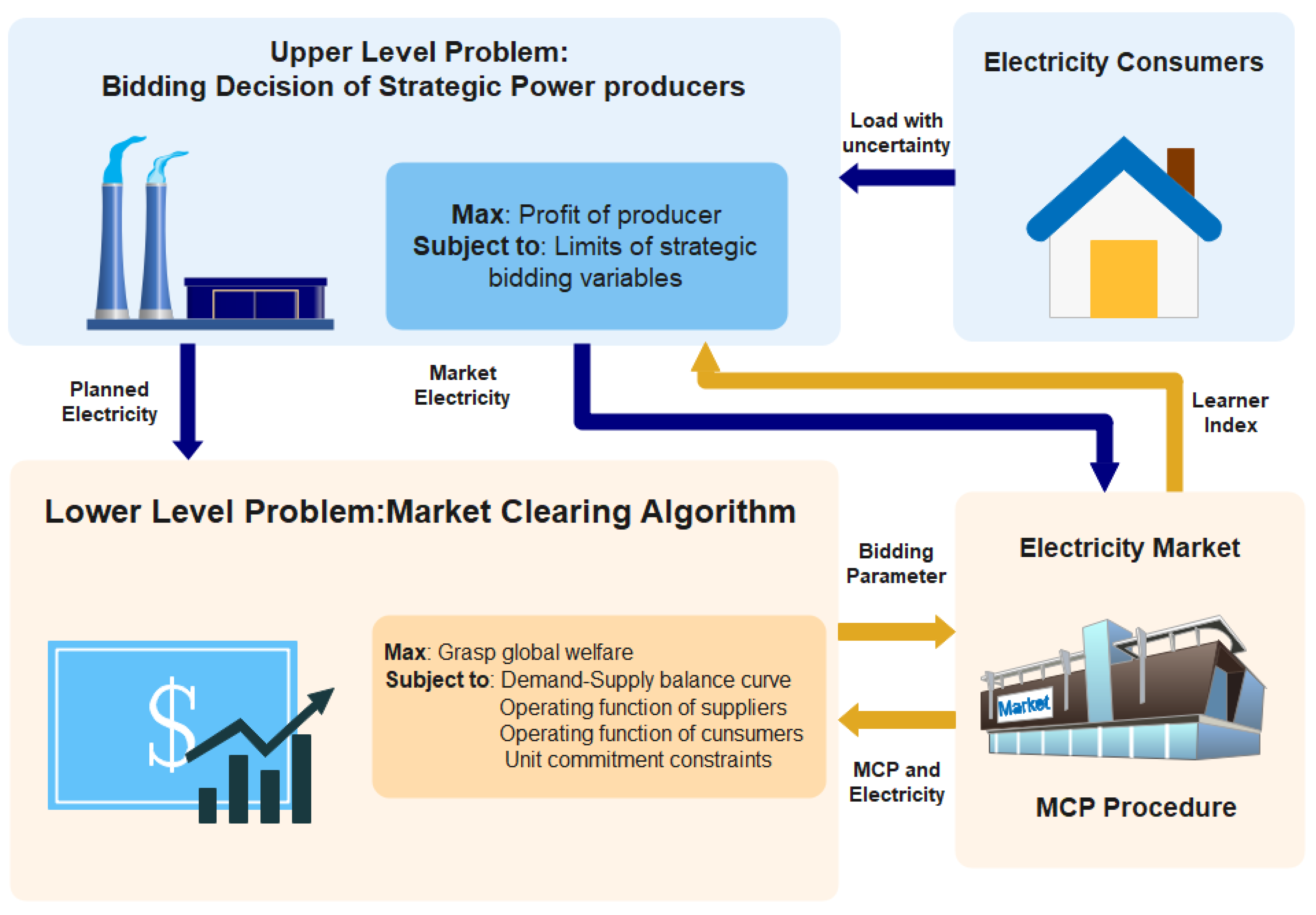
A generating company has run at a high degree of efficiency to flourish in a fierce competition. However, in the electricity sector, good execution may not be enough since, in order to generate the most profit, it must sell its products at a competitive price. Different factors affect a producing company’s profit, including its own bids, bids submitted by competitors, overall energy demands, and so on. Despite the fact that a generating company has no control over its competitors’ bids or the energy demand, it can create its own strategy for putting in a bid that maximizes profit while minimizing risk, as shown in Figure 3.

2.2. Mathematical Formulation

The market operator plots an upward production possibilities curve and a vertical line for consumer expectations following accepting offers from the Gen-Co’s. The point where the two curves intersect is the equilibrium point, and the straight line drawn from the equilibrium point on the y-axis determines the system’s MCP.

2.2.1. Objective Function

The profit of Gen-Co is calculated using the given (1).

$${Gen-Co}_{k,profit}=Revenue-{Gen-Co}_{k,cost}$$

(1)

here,

$$Revenue=MCP\times Q_k$$

(2)

$${Gen-Co}_{k,cost}=a_k{Q}_k+b_k{Q}_k^2$$

(3)

where, $Q_k$ is the amount of quantity of kth Gen-Co trade in the market. $a_k$ and $b_k$ are the cost coefficients.

2.2.2. Operating Constraints

i

Generation Limits

$$Q_{min}{U}_{k\left(t\right)}\le Q_{k\left(t\right)}\le Q_{max}{U}_{k\left(t\right)},\forall t\in T$$

(4)

ii

Inter-temporal constraints

$$(1-U_{k(t+1)})M_k^{ut}\le h_{k\left(t\right)}^{on},if{U}_{k\left(t\right)}=1.$$

(5)

$$U_{k\left(t+1\right)}{M}_k^{dt}\le h_{k\left(t\right)}^{off},if{U}_{k\left(t\right)}=0.$$

(6)

iii

Limits on bid price

$${C_{min}\le Gen-Co}_{k,cost}\le \overline{C}$$

(7)

3. Proposed Technique

3.1. Harris Hawks Optimization Algorithm: A Framework

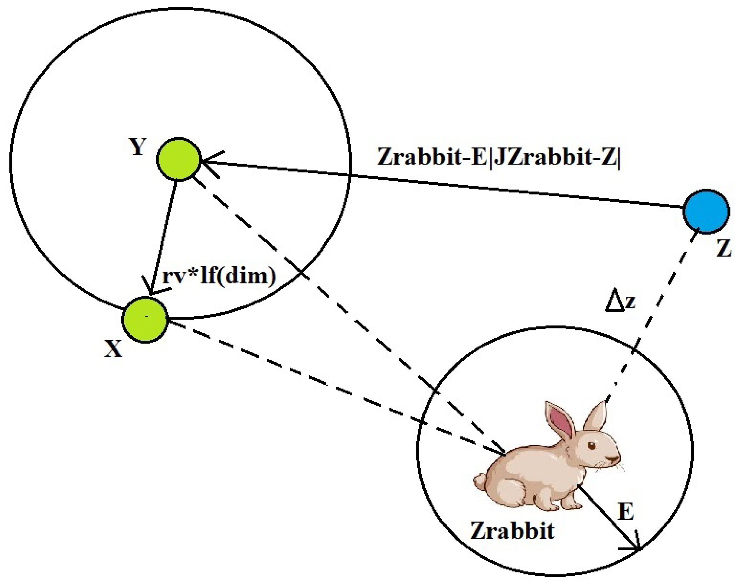
Ali Asghar Heidari et al. [11] presented the Harris Hawks Optimization (HHO) meta-heuristic algorithm in the year 2019. Harris hawks exhibit superb social behavior with respect to hunting and attacking the bunny. Searching for a bunny, hitting it in various ways, and executing a rapid jump are all part of the exploitative aspects of the technique. Harris hawks spread to various locations in search of rabbits, and they use two distinct investigating tactics. Aspirants are perhaps the intended prey or very close to it, with the targeted prey or really close to it being the ideal. Harris hawks perch in a spot similar to those of other families, as well as the bunny in the very first encounter (prey). The hawks in the second step look for tall trees randomly. The HHO then progresses an optimization process by mathematically faking such beneficial approaches and behaviors.

3.1.1. Initialization Step

At this step, the search space and objective function are defined. Furthermore, the first population-based chaotic maps are being developed. In addition, all of the attribute values have been specified.

3.1.2. The Step of Exploration

During this step, all Harris hawks are viable candidate responses. In each cycle, the fitness value is computed for each of these viable alternatives based on the desired prey. Two approaches have been introduced to replicate the exploring capabilities of Harris hawks in the search area, as specified in Equation (8).

$$z(i+1)=\left\{\begin{array}{c}{z}_r\left(i\right)-g_1\left|z_r\left(i\right)-2g_{2}z\left(i\right)\right|q\ge 0.5\\ (z_{rabbit}\left(i\right)-z_a\left(i\right))-g_3(lb+g_4(ub-lb))q<0.5,\end{array}\right.$$

(8)

The hawks’ positions within (ub-lb) borders are based upon two precepts: (1) create the responses using a hawk from the current population as well as other hawks randomly and (2) build outcomes based on the prey’s position, the average hawk’s location, and random weighted elements. Despite the fact that g3 is a scale parameter, if the value of r4 reaches one, it will help to boost the unpredictability of the algorithm. This law adds an arbitrarily scaled drive length to lb.

Additional dynamic capabilities to investigate other sections of the feature space are explored with a random scaled component. The average hawk posture (solutions) is stated as follows in Equation (9):

$$z_a\left(i\right)=\frac{1}{n}\sum _{l=1}^n{z}_l\left(i\right)$$

(9)

Once the hawk uses the random hawks’ information to catch the rabbit, rule 1 is usually applied in Equation (8). Rule 2 is executed once all hawks have accepted the finest hawk and the optimal option have been picked.

3.1.3. From Exploration to Exploitation Transition

This step depicts how HHO progresses from exploration to exploitation based on the bunny’s level of energy (E). The strength of the bunny is gradually depleted as a result of the bunny’s escaping behaviors, as according HHO. The energy needed decline is modeled in Figure 4.

E${}_0$ is the expected power decline, as shown in Equation (10).

$$E=2E_0\left(1-\frac{i}{I}\right),E_0\in [-1,1]$$

(10)

3.1.4. Step of Exploitation

In this step, the exploitation step is accomplished by employing four distinct factors. The position that was discovered during the exploration stage determines these strategies. Despite the hawks’ best efforts to track it down and catch it, the prey frequently sought to flee. To emulate the hawks’ offensive style, HHO exploitation employs four basic strategies. The four strategies are soft besiege, soft besiege with progressive speedy dives, hard besiege, and hard besiege with progressive speedy dives. These approaches are contingent on two variables, r and $\left|E\right|$, which label the technique to be cast-off. Where, $\left|E\right|$ is the prey’s escaping energy and r is the probability of escaping, with r < 0.5 indicating a better likelihood of the prey escaping effectively and r ≥ 0.5 representing an unsuccessful escape.

The following is an overview of these approaches:

• Soft besiege approach
  The rabbit has some energy to escape in the soft besiege method, where r ≥ 0.5 and $\left|E\right|$ ≥ 0.5, while the hawks are softly encircling the prey suddenly lost additional energy before completing the unexpected pounce. In Equations (11)–(13), soft besiege is described mathematically.

  $$z(i+1)=\Delta z\left(i\right)-E|j{z}_{rabbit}-z\left(i\right)|$$

  (11)

  $$\Delta z\left(i\right)=z_{rabbit}-z\left(i\right)$$

  (12)

  $$j-2(1-r_5),g_5\in [0,1]$$

  (13)
• Hard besiege approach
  The prey is so tired when r ≥ 0.5 and $\left|E\right|$$<$ 0.5 and at this time the escaping energy is very low. In addition, the Harris hawks scarcely encircle the planned prey to at long last play out the unexpected pounce. The present positions are updated in this condition by using Equation (14).

  $$z(i+1)=z_{rabbit}\left(i\right)-E|\Delta z\left(i\right)|$$

  (14)
  An easy instance of this step with one hawk is represented in Figure 5.
• Soft besiege approach with progressive speedy dives
  In this circumstance r$<$ 0.5 and $\left|E\right|$ ≥ 0.5, the rabbit has enough energy to flee. The hawks move astutely around the prey and calmly plunges before the amazed jump. The harris hawk’s position is refreshed in two stages throughout this action, which is referred to as adaptive soft besiege. In the initial stage, the harris hawks advance near the rabbit by assessing the following move of the rabbit as shown by Equation (15).

  $$y=z_{rabbit}\left(i\right)-E|j{z}_{rabbit}\left(i\right)-z\left(i\right)|$$

  (15)
  In the subsequent stage, the harris hawks concluded to jump, in view of the examination between the past jump and the conceivable outcome. In case it is not, the harris hawk delivers an unpredictable jump, based on the Levy Flight (LF) idea, as detailed in Equation (16).

  $$x=y+rv\times lf\left(Dim\right)$$

  (16)
  In Equation (16), the Dim represents the dimension of the solutions, rv is random vector of size 1 × $Dim$. lf is for the levy fight function and it is calculated using Equation (17).

  $$lf\left(z\right)=0.001\times \frac{u\times \sigma }{{\left|v\right|}^{\frac{1}{\beta }}},\sigma ={\left(\frac{\mathsf{\Gamma }(1+\beta )\times sin\left(\frac{\mathsf{\Pi }\beta }{2}\right)}{\mathsf{\Gamma }\left(\frac{1+\beta }{2}\right)\times \beta \times 2\left(\frac{\beta -1}{2}\right)}\right)}^{\frac{1}{\beta }}$$

  (17)

  where u, v are random values inside (0.1) and $\beta$ is a default constant and it is 1.5. In the soft besiege stage, Equation (11) can update the positions of hawks in the final strategy.

  $$x=\left\{\begin{array}{c}yiff\left(y\right)<f\left(z\right(i\left)\right)\hfill \\ xiff\left(x\right)<f\left(z\right(i\left)\right)\hfill \end{array}\right.$$

  (18)
  An example of this process for one hawk is shown in Figure 6. Sometimes during iterations, the position background of LF-based leapfrog trends is also documented and shown in this illustration. There is an LF-based trend in one trial, and the colored dots are the location footprints. It will only be possible to pick the best position Y or Z in every step. It is the same for all of the search agents.
• Hard besiege with progressive speedy dives
  The rabbit has not so much energy to escape at r $<$ 0.5 and $\left|E\right|$$<$ 0.5 and before the surprise pounce to capture and kill the prey, a hard besiege is constructed is shown in Figure 7.
  There are similarities between this step and the soft besiege, and yet this time, the hawks try to reduce one‘s average distance from the escaping prey. This is why it is necessary to follow all aspects when under hard besiege:

  $$x=\left\{\begin{array}{c}yiff\left(y\right)<f\left(z\right(i\left)\right)\hfill \\ xiff\left(x\right)<f\left(z\right(i\left)\right)\hfill \end{array}\right.$$

  (19)

  where, y and x are calculated using Equations (20) and (21).

  $$y=z_{rabbit}\left(i\right)-E|j{z}_{rabbit}\left(i\right)-z_a\left(i\right)|$$

  (20)

  $$x=y+rv\times lf\left(Dim\right)$$

  (21)

The procedure of the HHO algorithm is presented in Figure 8.

4. Deep Neural Network

Deep neural network is a machine learning discipline that focuses on understanding several levels of representations by creating a structure of features in which the top levels are described by the lower tiers, and the same lower tier features can be used to construct many top level features [27]. The relation between artificial intelligence, machine learning and deep learning is presented in Figure 9.

To describe more complicated and nonlinear relationships, the DL (Deep Learning) structure extends classic neural networks (NN) by adding more hidden layers to the network design between the input and output layers. This approach has piqued the interest of academics in recent years due to its superior performance in a variety of EM applications [28,29,30]. Convolutional-Neural Networks (C-NN) have become a popular DL design in recent years because they can perform sophisticated functions using convolution filters. Another DL design that is commonly used for classification or regression with success in many areas is the Deep Neural Network (DNN). It is a common feed forward network in which the input passes from the input layer to the output layer via a number of hidden layers that exceed two [30]. The usual design for DNNs is shown in Figure 10, where Ni is the input layer, which contains neurons for input features, No is the output layer, which contains neurons for output classes, and Nh,l are the hidden layers.

5. Harris Hawk Optimization of Deep Neural Networks Architecture

Figure 11 shows the general framework of the suggested model for estimating the optimal bids in EM. The suggested model’s main goal is to improve the performance of the NN by applying the HHO algorithm to discover the ideal NN weights, hence the name HHO-NN. The suggested HHO-NN begins by determining the beginning value for a group of N individuals X. Each of these individuals represents the NN weights, thus we have a collection of N networks from which to choose the best. As a result, the data set is randomly divided into training and testing sets of 70% and 30% respectively.

The training data set is used to analyse the existing network’s (solution) effectiveness by determining the corresponding objective function, which is dependent on the original value yi and the forecast value y.

$$fit=\sqrt{\frac{{\sum }_{l=1}^{ns}{y}_l-{\widehat{y}}_l}{ns}}$$

(22)

The next phase is to locate the network, Yb, with the lowest fitness value. Then, using the optimal solution and the HHO’s operation, the other solutions will be modified. When the stopping circumstances are achieved, the process of updating solutions and determining the best option will be completed. The test set is used to determine the quality of the output to evaluate the performance of the best network developed during the training phase.

6. Simulation Results and Experimentation

The variation is written in MATLAB 2019 and operates on a 4.00 GHz i5 processor with 8 GB of RAM. The number of iterations and population size for all algorithms are kept constant in order to draw an evaluation of optimization routines (i.e., maximum number of iterations = 500 and number of search agents = 50).

To test the forecasting potential of the ANN version, extraordinary criteria are used. This potential can be checked after the MCP is calculated. The four types of errors are checked in this, which are the root mean of squared error (RMSE), the mean absolute error (MAE), the mean absolute percentage error (MAPE) and the coefficient of co-relation (CC).The performance result of these tests is shown in

Table 1. Performance Test Results.

Model	Performance Test Result
	MAE (m)	MAPE (%)	RMSE (m)	CC
Training Period
ALO-NN	0.286	49.369	0.3054	0.9154
GWO-NN	0.21	45.658	0.2721	0.9514
SCA-NN	0.268	48.246	0.3012	0.9264
WOA-NN	0.254	46.565	0.2748	0.9421
HHO-NN	0.179	42.124	0.2541	0.9668
Testing Period
ALO-NN	0.281	35.61	0.2967	0.8755
GWO-NN	0.204	31.74	0.2682	0.8977
SCA-NN	0.258	35.87	0.2964	0.8869
WOA-NN	0.249	32.54	0.2699	0.8013
HHO-NN	0.177	28.87	0.252	0.821

Regression verification of the proposed algorithm was also undertaken to check the validation of the same.

• Mean Absolute Error (MAE)
  The MAE is the average of the absolute values of the forecasting error and s calculated with Equation (23).

  $$MAE=\frac{1}{1000}\sum _{i=1}^{1000}\left|f_i-{\hat{f}}_i\right|$$

  (23)
• Mean Absolute Percentage Error (MAPE)
  The mean absolute percentage error is usually taken as a loss function for solving the problem of regression and in evaluation of model because of its very instinctive clarification in terms of relative error, as shown in Equation (24).

  $$MAPE=\frac{1}{1000}\sum _{i=1}^{1000}\left|\frac{f_i-{\hat{f}}_i}{f_i}\right|\times 100$$

  (24)
• Root Mean Square Error (RMSE)
  The RMSE is defined as the square root of the second sample moment of the differences between predicted and actual data. RMSE is shown in Equation (25).

  $$RMSE=\sqrt{\frac{1}{1000}\sum _{i=1}^{1000}{(f_i-{\hat{f}}_i)}^2}$$

  (25)
• Coefficient of Co-relation (CC)
  To determine the strength of a relationship between data, correlation coefficient formulas are utilized as shown in Equation (26). The formulas return a number between −1 and 1, with the following values:

  -

  A strong positive association is indicated by a value of one.

  -

  A negative association is indicated by a value of −1.

  -

  A zero means that there is no connection at all.

  $$CC=\frac{{\displaystyle \sum _{i=1}^{1000}}({\hat{f}}_i-{\overline{\hat{f}}}_i)(f_i-{\overline{f}}_i)}{\sqrt{{\displaystyle \sum _{i=1}^{1000}}{({\hat{f}}_i-{\overline{\hat{f}}}_i)}^2{\displaystyle \sum _{i=1}^{1000}}{(f_i-{\overline{f}}_i)}^2}}$$

  (26)

• Regression Verification Regression verification is the practice of ensuring that no significant errors have been created in the algorithm after the adjustments have been made by testing the altered sections of the code as well as the parts that may be affected by the modifications shown in Figure 12.
• A fair comparison has been made between different optimization algorithm tuned neural networks such as GWO-NN, ALO-NN, SCA-NN, WOA-NN and HHO-NN on the basis of error indices calculations, here we have reported MSE, RMSE and MAE values of the prediction it has been observed that proposed architecture yields the least errors in training and testing mode.

7. Application of HHO-NN on Optimal Bidding Challenge of Electricity Market

IEEE-14 bus test system is taken, where, three competing generating companies compete with Gen-Co-G. The competition is for selling power in EM, the bidding strategy is designed for optimum output.

Table 2. Rival’s Bidding Data for IEEE-14 Bus System [30].

Blocks	Q/Std. Dev./Mean	R1	R2	R3
Block I	Q (MW)	200	150	150
	Std. Dev. ($/MWh)	2	3	2
	Mean ($/MWh)	9	11	10
Block II	Q (MW)	120	120	140
	Std. Dev. ($/MWh)	3	2	3
	Mean ($/MWh)	15	17	18
Block III	Q (MW)	100	120	100
	Std. Dev. ($/MWh)	2	3	3
	Mean ($/MWh)	19	18	17
Block IV	Q (MW)	120	130	120
	Std. Dev. ($/MWh)	2	3	2
	Mean ($/MWh)	21	25	26
Block V	Q (MW)	50	45	40
	Std. Dev. ($/MWh)	2	3	3
	Mean ($/MWh)	27	32	25

shows the bid data of competitor prices and

Table 3. Power Blocks data of Gen-Co-G for IEEE-14 Bus System [30].

Block	${\mathit{c}}_0$ ($/MW2H)	${\mathit{c}}_{\mathit{I}}$ ($/MWH)	${\mathit{c}}_{\mathit{I}\mathit{I}}$ ($/H)	${\mathit{P}}_{\mathit{m}\mathit{a}\mathit{x}}$	${\mathit{P}}_{\mathit{m}\mathit{i}\mathit{n}}$	MUT	MDT	${\mathit{C}}_{\mathit{h}\mathit{s}}$	${\mathit{C}}_{\mathit{c}\mathit{s}}$	${\mathit{t}}_{\mathit{c}}$	${\mathit{c}}_{\mathit{n}}^{\mathit{s}\mathit{d}}$
Block I	0.00375	2	0	250	10	1	1	70	176	1	50
Block II	0.0175	1.75	0	140	20	2	1	74	187	1	60
Block III	0.0625	1	0	100	15	1	1	50	113	1	30
Block IV	0.00834	3.25	0	120	10	1	2	110	267	1	85
Block V	0.025	3	0	45	10	1	1	72	180	4	52

shows the power-blocks data of Gen-Co-G [30].

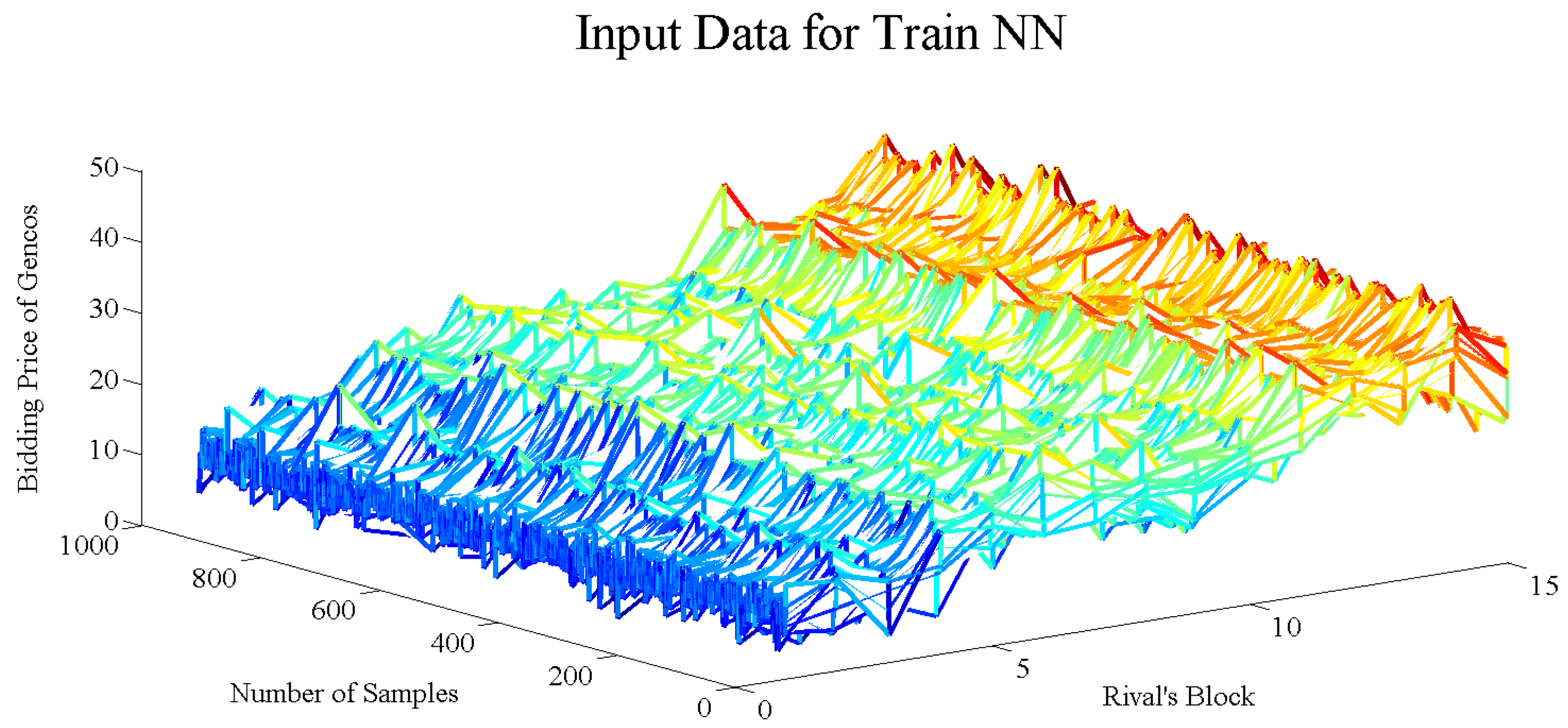
For constructing the neural network, we have generated 1000 samples for preparing the HHO-NN, out of these data, 70% has been used for training and the remaining 15% has been kept for validation purposes. We report the results of some unknown samples in this analysis. A toal fo ten unknown samples were taken and the analysis of these samples is depicted through Figure 13 and Figure 14 are the input and target data to train the NN. The input data to train the NN for the strategic bidding problem in EM are competitors’ bidding data and the target data are profit of Gen-Co-G for the same inputs.

Figure 15 represents the input data for testing the trained NN for the specific problem of attaining the optimal bids and optimal profit of the Gen-Co-G in the EM.

Figure 16 represents the profit curve obtained by the selected algorithms. From the figure, it can be observed that the proposed supervised net yields maximum profit as compared to other Monte Carlo-based optimization approaches. The cumulative profit calculated by this architecture is ($153,275). However, the profit calculated by HHO is ($138,758.75), ALO-NN is ($128,543.42), GWO-NN is ($117,641), MFO-NN is ($121,051), ALO is ($80,176.20458), GWO is ($126,070.0738), SSA is ($86,375.01205) and WOA is ($119,826.25). This is due to the better anticipating capability of market conditions by the HHO tuned neural network.

8. Conclusions and Future Scope

The proposed Harris Hawk Optimization-based Deep Neural Networks Architecture is used to investigate the optimum bidding strategy problem in the power market. Using the expected load and competitors’ bidding data, the planned architecture determines the best bidding technique for maximising the profit. For various power demand values, provider end income, customer end profit, and MCP values, the proposed methodology is examined. IEEE 14 is used to dissect the viability of the suggested technique in the MATLAB/Simulink platform. The proposed approach displays excellent productivity by combining the relative examination with alternate techniques such as ALO-NN, GWO-NN, MFO-NN, ALO, GWO, SSA, WOA and standard HHO.

The proposed calculations have the advantages of reduced computational complexity and good accuracy in extrapolating subjective data. Furthermore, the proposed work’s statistical measurements such as mean and standard deviation, as well as performance metrics such as best, worst, average, and computational time, were validated. It was demonstrated that the proposed methodology outperformed other strategies in terms of statistical measures when compared to methodologies for comparing results.

Furthermore, the investigations on the bigger network with multiple players and more constraints pertaining to generation, transmission limits, transmission congestion and consumer side bidding, will be addressed in our future publications.

References

- Zaman, F.; Elsayed, S.M.; Ray, T.; Sarker, R.A. Co-evolutionary approach for strategic bidding incompetitive electricity markets. Appl. Soft Comput. 2017, 51, 1–22. [Google Scholar] [CrossRef]
- Sandhu, H.S.; Fang, L.; Guan, L. Forecasting day-ahead price spikes for the Ontario electricity market. Electr. Power Syst. Res. 2016, 141, 450–459. [Google Scholar] [CrossRef]
- Girish, G.P. Spot electricity price forecasting in Indian electricity market using autoregressive-Garch models. Energy Strategy Rev. 2016, 11–12, 52–57. [Google Scholar] [CrossRef]
- Abedinia, O.; Amjadi, N.; Shafie-Khah, M.; Catalao, J.P.S. Electricity price forecast using combinatorial neural network trained by a new stochastic search method. Energy Convers. Manag. 2015, 105, 642–654. [Google Scholar] [CrossRef]
- Grilli, L. Deregulated Electricity Market and Auctions: The Italian Case; Scientic Research an Academic Publisher: Wuhan, China, 2010; Volume 2, pp. 238–242. [Google Scholar]
- Bunn, D.W. Forecasting loads and prices in competitive power markets. IEEE Xplore 2000, 88, 163–169. [Google Scholar] [CrossRef]
- Girish, G.P.; Rath, B.N.; Akram, V. Spot electricity price discovery in Indian electricity market. Renew. Sustain. Energy Rev. 2018, 82, 73–79. [Google Scholar] [CrossRef]
- Khosravi, A.; Nahav, I.S.; Creighton, D. A neural network-GARCH-based method for construction of prediction intervals. Electr. Power Syst. Res. 2013, 96, 185–193. [Google Scholar] [CrossRef]
- Janczura, J.; Truck, S.; Weron, R.; Wol, R.C. Identifying spikes and seasonal components in electricity spot price data: A guide to robust modeling. Energy Econ. 2013, 38, 96–110. [Google Scholar] [CrossRef] [Green Version]
- Heidari, A.A.; Mirjalili, S.; Faris, H.; Aljarah, I.; Mafarja, M.; Chen, H. Harris hawks optimization: Algorithm and applications. Future Gener. Comput. Syst. 2019, 97, 849–872. [Google Scholar] [CrossRef]
- Tharani, S.; Yamini, C. Classification using convolutional neural network for heart and diabetics data-sets. Int. J. Adv. Res. Comput. Commun. Eng. 2016, 5, 417–422. [Google Scholar]
- Jiao, S.; Wang, C.; Gao, R.; Li, Y.; Zhang, Q. Harris Hawks Optimization with Multi-Strategy Search and Application. Symmetry 2021, 13, 2364. [Google Scholar] [CrossRef]
- Nogales, F.J.; Contreras, J.; Conejo, A.J.; Espinola, R. Forecasting next-day electricity prices by time series models. IEEE Trans. Power Syst. 2002, 17, 342–348. [Google Scholar] [CrossRef]
- Zhang, J.; Tan, Z.; Yang, S. Day-ahead electricity price forecasting by a new hybrid method. Comput. Ind. Eng. 2012, 63, 695–701. [Google Scholar] [CrossRef]
- Yang, Z.; Ce, L.; Lian, L. Electricity price forecasting by a hybrid model, combining wavelet transform. ARMA and kernel-based extreme learning machine methods. Appl. Energy 2017, 190, 291–305. [Google Scholar] [CrossRef]
- Khashei, M.; Rafiei, F.M.; Bijari, M. Hybrid fuzzy auto-regressive integrated moving average (FARIMAH) model for forecasting the foreign exchange markets. Int. J. Comput. Intell. Syst. 2013, 6, 954–968. [Google Scholar] [CrossRef] [Green Version]
- Qi, Y.; Liu, Y.; Wu, Q. Non-cooperative regulation coordination based on game theory for wind farm clusters during ramping events. Energy 2017, 132, 136–146. [Google Scholar] [CrossRef] [Green Version]
- Lago, J.; De Ridder, F.; Vrancx, P.; de Schutter, B. Forecasting day-ahead electricity prices in Europe: The importance of considering market integration. Appl. Energy 2018, 211, 890–903. [Google Scholar] [CrossRef]
- Gholipour Khajeh, M.; Maleki, A.; Rosen, M.A.; Ahmadi, M.H. Electricity price forecasting using neural networks with an improved iterative training algorithm. Int. J. Ambient. Energy 2018, 39, 147–158. [Google Scholar] [CrossRef]
- Bento, P.M.R.; Pombo, J.A.N.; Calado, M.R.A.; Mariano, S.J.P.S. A bat optimized neural network and wavelet transform approach for short-term price forecasting. Appl. Energy 2018, 210, 88–97. [Google Scholar] [CrossRef]
- Aggarwal, S.K.; Saini, L.M.; Kumar, A. Electricity price forecasting in deregulated markets: A review and evaluation. Int. J. Electr. Power Energy Syst. 2009, 31, 13–22. [Google Scholar] [CrossRef]
- Singhal, D.; Swarup, K.S. Electricity price forecasting using artificial neural networks. Int. J. Electr. Power Energy Syst. 2011, 33, 550–555. [Google Scholar] [CrossRef]
- Mandal, P.; Senjyu, T.; Funabashi, T. Neural networks approach to forecast several hour ahead electricity prices and loads in deregulated market. Energy Convers. Manag. 2006, 47, 2128–2142. [Google Scholar] [CrossRef]
- Pao, H.-T. Forecasting electricity market pricing using artificial neural networks. Energy Convers. Manag. 2007, 48, 907–912. [Google Scholar] [CrossRef]
- Ostadi, B.; Sedeh, O.M.; Kashan, A.H. Risk-based optimal bidding patterns in the deregulated power market using extended Markowitz model. Energy 2020, 191, 116516. [Google Scholar] [CrossRef]
- Kavita, J.; Saxena, A. Evolutionary Neural Network based hybrid architecture for strategic bidding in electricity market. In Proceedings of the 2021 IEEE 2nd International Conference on Smart Technologies for Power, Energy and Control (STPEC), Bilaspur, India, 19–22 December 2021. [Google Scholar]
- Anbazhagan, S.; Kumarappan, N. Day-ahead deregulated electricity market price classification using neural network input featured by DCT. Int. J. Electr. Power Energy Syst. 2012, 37, 103–109. [Google Scholar] [CrossRef]
- Li, Y.; Yu, N.; Wang, W. Machine learning-driven virtual bidding with electricity market efficiency analysis. IEEE Trans. Power Syst. 2021, 37, 354–364. [Google Scholar] [CrossRef]
- Angulo, A.; Rodríguez, D.; Garzón, W.; Gómez, D.F.; Al Sumaiti, A.; Rivera, S. Algorithms for Bidding Strategies in Local Energy Markets: Exhaustive Search through Parallel Computing and Metaheuristic Optimization. Algorithms 2021, 14, 269. [Google Scholar] [CrossRef]
- Tahir, M.F.; Saqib, M.A. Optimal scheduling of electrical power in energy-deficient scenarios using artificial neural network and Bootstrap aggregating. Int. J. Electr. Power Energy Syst. 2016, 83, 49–57. [Google Scholar] [CrossRef]