Optimizing Cybersecurity Investments over Time

Abstract

In the context of growing vulnerabilities, cyber-risk management cannot rely on a one-off approach, instead calling for a continuous re-assessment of the risk and adaptation of risk management strategies. Under the mixed investment–insurance approach, where both risk mitigation and risk transfer are employed, the adaptation implies the re-computation of the optimal amount to invest in security over time. In this paper, we deal with the problem of computing the optimal balance between investment and insurance payments to achieve the minimum overall security expense when the vulnerability grows over time according to a logistic function, adopting a greedy approach, where strategy adaptation is carried out periodically at each investment epoch. We consider three liability degrees, from full liability to partial liability with deductibles. We find that insurance represents by far the dominant component in the mix and may be relied on as a single protection tool when the vulnerability is very low.

1. Introduction

Cybercrime costs exhibit a continuous growth trend, with a 15% year-on-year increase (See the estimate by Cybersecurity Ventures on https://cybersecurityventures.com/cybercrime-damage-costs-10-trillion-by-2025/, (accessed on 15 May 2022)). A faster-than-exponential growth was observed in the years from 2000 to 2006 [1]. Later, an investigation into breaches up to 2015 reported an increase in the overall frequency of large data breaches [2]. Finally, a steady increase of cyber-incidents was noted in the years up to 2018 in [3]. Though most cybersecurity literature is devoted to analyzing vulnerabilities and their reduction, the sheer growth of cyber-risk threats calls for a broader range of countermeasures, which do not involve just the engineering side.

The panorama of risk-management techniques includes risk transfer (e.g., insurance) and risk avoidance in addition to risk mitigation (with the latter category essentially incorporating all the technical countermeasures). The classification of strategies adopted for cyber-risk management is not different from what is considered for general risk management [4,5,6]. It is to be considered that, though risk avoidance is typically included in the set of risk-management strategies, is not a viable option in many cases, since it could lead to a significant sacrifice of usability [7]. A historical survey of cyber-risk management is provided by [8].

After the early debate on the insurability of cyber-risks [9], a market for insurance has actually developed [10,11,12,13]. Pricing methods have been proposed to compute the insurance premium (see, e.g., [14]).

More recently, a new approach, based on the joint use of risk mitigation and risk transfer measures, has been proposed [15,16]. In that approach, investments allow us to reduce the vulnerability, which in turn is reflected in a lower premium. So far, those investigations have considered investments in security as a one-off option. However, the reality is that companies must keep investing in security to confront new threats. The net effect of the evolving landscape is a natural growth of vulnerability over time. A logistic model has been recently proposed in [17] to describe that growth. The joint mitigation-transfer approach must be reassessed in this context of growing vulnerability.

In this paper, we approach the problem of devising a joint risk-management approach in the face of a growing vulnerability by looking for the optimal investment amount to minimize the overall security expense (investment plus insurance) when threats keep growing and call for a sequence of investments. Here, we adopt a greedy approach where optimization is sought at each investment step rather than globally over a time horizon. Our major contribution is evaluating the optimal investment for a sequence of epochs when insurance and investment are employed jointly for three insurance liability cases (full liability, partial liability, and partial liability with deductibles).

After the literature review in Section 2, we describe the models employed for the effectiveness of investments and vulnerability growth over time in Section 3. The investment optimization problem is posed in Section 4 and solved in Section 5 for the scenario where investments are carried out periodically. Finally, in Section 6, we report some results.

2. Literature Review

In this paper, we deal with a problem in cyber-risk management. We can classify the literature of interest about this topic into four primary groups: those sketching a general cyber-risk management framework; those describing the mitigation approach by identifying a relationship between investments in security and vulnerability; those analyzing the pricing proposition in insurance; and those considering a mixed investment–insurance approach.

A general taxonomy of risk-management approaches is contained in the recent paper by Eling et al. [8]. In the class of papers describing a general framework to address cyber-risks, a major subclass is represented by those papers concerning critical infrastructures, where the subject of risk interdependence is particularly relevant. That dependence is described in [18], where the growing importance of cyber-risks is highlighted. In order to decide which approach to use in the toolbox of risk management (including tolerance), Kure et al. propose a scoring system coupled with a decision tree [19].

The most established model to relate security investments and vulnerability reduction, which allows us to compute the optimal investment to be made in security, is due to Gordon and Loeb (GL) [20], who actually proposed two models, which we refer to as GL1 and GL2 in the following. The use of GL models in a practical setting has been investigated in [21,22]. A special form of the GL1 model was derived by [23] when attacks target a particular node (one-to-one attacks) (the equivalence of the two models was proven by [24]). The GL1 model has been used in several papers [25,26,27,28,29], and a dynamic extension has also been proposed by [30]. For the GL2 model also, an equivalent model was derived in [23] to model attacks that propagate epidemically over a scale-free network (opportunistic attacks). The equivalence of the GL2 model and that proposed by [23] was proven by [24]. The GL2 model was used, e.g., by [15,16,25,28,29,31,32,33].

Three additional models to describe the impact of investments on the breach probability have been proposed in [34]. Additionally, three more models, respectively named the exponential power class function, the proportional hazard class model, and the Wang transform model, have been proposed in [35]. The exponential power class function has been employed by [36] to derive an optimal mix of mitigation measures and investments in knowledge and expertise. All the three models proposed by Wang have been employed by [37] to investigate the competition between two cloud providers.

The economic consequences of cyberattacks have also been a matter of concern for a long time, as shown in the cyber-risk management framework proposed by [38]. A taxonomy has been proposed to classify the costs of cybercrime [39]. The consequences on the market value of companies must be accounted for in addition to the direct losses suffered by companies and their customers [40,41]. Of course, the ultimate goal is to estimate the actual costs, which is the subject of several papers, e.g., [26,42,43,44,45].

The decision to invest may also be related to the risk-taking attitude of the company [25]. However, not investing enough in security may lead to liability consequences as well [24]. Though most papers adopt a straightforward net profit maximization approach, a mixed-integer linear programming formulation has been adopted in [32] for an Industry 4.0 supply chain. A game-theoretic approach is employed in [29] to analyze the investment strategies of two interconnected firms under different types of attack (targeted vs opportunistic). A similar context has been further explored in [33], where a company with systems deployed both in its headquarters and some branches has been considered. The optimal trade-off between investing in knowledge and expertise versus investing in deploying mitigation measures has been investigated by [36]. A different approach is taken in [46], where a stochastic programming approach is employed to minimize the overall cybersecurity expense under the use of investments only, considering a time-varying investment effectiveness described by an exponential function of the investment.

A risk-management tool alternative to investing in cybersecurity is insurance. Insurance is a risk transfer measure whereby the insured is indemnified against cybersecurity-related losses by paying a periodic fixed sum (the premium). The actuarial approach is a more recent streak in cyber-risk management. A thorough discussion of pricing principles (premium setting) as well as a brief review of frequency and severity models for security breaches are contained in [14]. An earlier survey of cyber insurance models is reported in the paper by [47], while a brief review of the state of the cyber insurance market is contained in [13], with similar analyses carried out for Sweden [10], Norway [12], and the US [11]. However, the debate about the use of insurance has gone on for several years, with contrasting opinions. For example, opinions favoring cyber insurance appeared in the papers by [48,49,50] (if protection quality is not high). On the other hand, insurance has also been considered a possible factor favoring a market for lemons. Opinions contrary to insurance are shown in [51,52], where the intrinsic information asymmetry concerning the insured’s vulnerability may lead to no insurance market. Additionally, the danger of overpricing insurance policies exists, since the insurer may have imperfect knowledge of risks and may err on the safer side [53,54]. Several approaches have been proposed to compute the premium. A mean-variance approach has been employed in [55]. A more accurate formula, which, however, requires the knowledge of skewness and kurtosis, has been proposed by [56]. The incorporation of a discount in premium formulas has been proposed in [15] to incentivize all actions aimed at reducing the amount of loss. That proposal has been advocated by [31] for the power sector. Additionally, security audits to design insurance contracts have been proposed in [57]. Since insurance may be reflected in the prices operators charge for their services, the issue of insurance price sustainability also arises [58]. The issue of correlated risks has been dealt with in [59] by resorting to a copula model.

Despite being sometimes presented as alternatives, investing in security and buying an insurance policy may be used together, as illustrated in the paper by [60]. Precisely, investing may be used to reduce the insurance premium, as advocated in several papers. The seminal paper in this context is probably that by Young et al. [15], where a pricing formula has been proposed that incorporates an incentive for vulnerability reduction. That same approach has been suggested in [61], where a risk assessment method based on the use of Bayesian attack graphs has been proposed. However, it has been shown that the mixed strategy may revert to insurance alone under certain conditions (e.g., low potential loss, or either very low or very high vulnerability), and optimal investment decisions may require an accurate estimate of the vulnerability [16].

3. Vulnerability, Investments, and Insurance

We consider a system exposed to cyberattacks, which can end up with a loss of money. Here we are not so much interested in quantifying the money lost due to those attacks, but the probability that the attack is successful, i.e., the probability that a data breach occurs. We call that probability the vulnerability $v(·)$ of the system, following the definition in [62]. In this section, we review the notion of vulnerability and describe how it varies under the influence of time and security expenses.

We consider data breaches as incidents where an attacker takes (steals) information from a system without the knowledge or authorization of the system’s owner. Consistent definitions of data breaches are employed in [20,34,35] The vulnerability is the probability that a data breach occurs, conditional on the risk event (see the definition 1.19 of [62]). The intention of the attacker to initiate an attack represents the threat (see the definition 1.18 of [62]).

If no money is spent on security, the vulnerability of a system naturally increases over time, since new threats are devised, and the shielding capability of the protection tools in place decays. Following the work of [17], we assume that a logistic function describes the shape of the time-led evolution of the vulnerability.

However, we can fight the natural growth of vulnerability by adopting either (or both) approaches to risk management, i.e., taking a risk mitigation policy or a risk transfer one. Risk mitigation is typically achieved by investing in security tools (e.g., antivirus software). Risk transfer consists instead of subscribing to an insurance policy that indemnifies us against the possible losses due to a cyberattack.

With risk mitigation, the vulnerability decreases as a function of the investment we carry out in security, though it cannot be reduced to zero. Though several functions have been proposed to describe the impact of investments on vulnerability, the two seminal models by Gordon and Loeb [20] are still the most widely employed ones. In the following, we refer to those models, respectively, as GL1 and GL2 for short.

Since we are interested in examining how the vulnerability evolves over time, we do not assume that investments take place on a single date. Instead, we have a sequence of times $t_0,t_1,t_2,\dots ,t_n$, with $z_i$ being the investment at time $t_i$. We envisage therefore a sawtooth-like vulnerability, which grows within each $(t_{i-1},t_i)$ interval due to time but is slashed after investments take place at times $t_1,t_2,\dots ,t_n$. The logistic function describing the evolution during no-investment intervals is then

$$v\left(t\right)=\frac{V}{1+e^{-k(t-a)}}{t}_i<t<t_{i+1}$$

(1)

where V is the maximum vulnerability value, k is the logistic growth rate or steepness of the curve, and the parameter $a=t_i+\frac{1}{k}ln\left[\frac{V}{v\left(t_i\right)}-1\right]$ is a function of the vulnerability value after the latest investment.

Under the GL1 model, after the $z_i$ investment, the vulnerability decreases to

$$v\left(t_i\right)=\frac{V}{{(1+\alpha z_i)}^{\beta }[1+e^{-k(t_i-a)}]}$$

(2)

If the GL2 model is adopted instead, the vulnerability decreases to

$$v\left(t_i\right)={\left[\frac{V}{1+e^{-k(t_i-a)}}\right]}^{\alpha z_i+1}$$

(3)

In Figure 1, we see the impact of investments in reducing the vulnerability despite its growth over time. In that case, we have considered a GL1 model with two investment events of EUR 10,000 each. You can see that the periodic reduction of vulnerability makes the overall vulnerability evolution resemble a sawtooth.

The risk transfer approach can be adopted as an alternative to risk mitigation. In this case, we may buy an insurance policy, pay the premium, and be indemnified against the potential loss. Though several papers have been devoted to the computation of the fair premium (see, e.g., Ref. [56] for more precise computation of the premium under the expected utility framework, or [33] for the case of a multi-branch company), we consider a simple expression, proposed in [39], where the premium P incorporates an incentive to invest in security (since investing decreases the probability of security breaches and the associated losses) as

$$P_i=P_0\left[1-r\left(1-v_i\right)\right]$$

(4)

where $P_0$ is the base premium rate, i.e., the premium in the total absence of investments, the vulnerability at time i is $v_i=v\left(t_i\right)$ after the i-th investment, and r is the discount factor. As in [16], we can assume that the base rate premium $P_0$ is a fraction $\gamma$ of the potential loss $\lambda$ as $P_0=\gamma \lambda q$, with q being the probability that an attack takes place.

We can consider variants of this scheme based on introducing liability limits. In addition to full liability (where the insurer insures the full loss suffered by the insured), we can consider an upper limit ℓ on the coverage: the insurer will refund the insured up to the amount ℓ. Should the actual loss $\lambda$ be larger than the maximum liability L, the insured will suffer a net loss $\ell -\lambda$. Finally, we can introduce a limit on liability from below in the form of deductibles. The deductible is the amount F paid out of pocket by the insured before the insurer pays any expenses. The compensation actually paid by the insurer when the loss due to the security breach is $\lambda$ will be $\lambda -F$. The rationale for deductibles is that they are meant to deter the many claims that could otherwise be submitted. Summing up, we consider three liability schemes:

• full liability;
• limited liability (with upper limit)
• limited liability with deductibles (both lower and upper limit).

Since the premium is set to incentivize investment, it is natural to consider mixed policies, where a company uses both mitigation and transfer tools by investing in security and buying insurance policies at the same time. Such a mixed policy has been shown to reduce the overall security expense to achieve the desired level of security [33].

4. The Security Expense Minimization Problem

As hinted at in Section 3, we consider a mixed strategy, where the company wishing to edge against cybersecurity-related losses invests in security and buys cybersecurity insurance at the same time. The company’s expense in security consists of both components. In this section, we provide a mathematical formulation of those components and define the security expense minimization problem.

In the following, we assume that the probability q of an attack does not depend on the specific epoch but just on the duration of the time interval $[t_i,t_{i+1}]$. For the time being, we assume that investment is carried out periodically so that $t_{i+1}-t_i=T,\forall i$. We also assume that the loss $\lambda$ in the case of a successful attack is a fixed quantity (this is quite a simplifying assumption, though the modeling of severity for security breaches calls for a probability density function model [39]).

In the case of full liability, the company invests in security and buys an insurance policy covering any loss at the same time. The overall expense is simply the sum of two components (investment and insurance premium):

$$E^{\mathrm{full}}=Z+P,$$

(5)

where $Z={\sum }_i^n{Z}_i$ is the overall investment throughout the n periods, and $P={\sum }_i^n{P}_i$ is similarly the sum of the insurance premiums paid over the periods. In particular, by recalling Equation (4), at the i-th period we have

$$E_i^{\mathrm{full}}=Z_i+P_0\left[1-r\left(1-v_i\right)\right],$$

(6)

where $v_i=v\left(t_i\right)$.

Similarly, if the insurance policy includes an upper limit u on liability, the overall expense will be

$$E^{\mathrm{partial}}=\left\{\begin{array}{c}Z+P\mathrm{if}\lambda \le u\hfill \\ Z+P+R\mathrm{if}\lambda >u\hfill \end{array}\right.$$

(7)

where q is the probability that an attack takes place, and $R={\sum }_{i=1}^n{R}_i$ is the residual loss not covered by insurance.

For the i-th period, the residual loss is

$$R_i=q(\lambda -u){\overline{v}}_i,$$

(8)

where ${\overline{v}}_i$ is the average vulnerability in $[t_i,t_{i+1}]$, since we must take into account that the timing of the data breach is unknown, and the probability of its success changes along the interval till the next investment instalment. After recalling Equation (1), we obtain

$${\overline{v}}_i=\frac{1}{t_{i+1}-t_i}{\int }_{t_i}^{t_{i+1}}v\left(t\right)dt=\frac{V}{kT}ln\left[1+\frac{v_i}{V}\left(e^{kT}-1\right)\right]$$

(9)

The expense in the i-th period is then

$$E_i^{\mathrm{partial}}=\left\{\begin{array}{c}{Z}_i+P_0\left[1-r\left(1-v_i\right)\right]\mathrm{if}\lambda \le u\hfill \\ Z_i+P_0\left[1-r\left(1-v_i\right)\right]+q(\lambda -u)\frac{V}{kT}ln\left[1+\frac{v_i}{V}\left(e^{kT}-1\right)\right]\mathrm{if}\lambda >u\hfill \end{array}\right.$$

(10)

We can now consider the third case, where we have both a lower bound ℓ and an upper bound u on liability. We refer to this case as partial liability with deductibles. The overall expense in the i-th period is then

$$E_i^{\mathrm{deduct}}=\left\{\begin{array}{cc}{Z}_i+P_0\left[1-r\left(1-v_i\right)\right]+\lambda q\frac{V}{kT}ln\left[1+\frac{v_i}{V}\left(e^{kT}-1\right)\right]\hfill & \mathrm{if}\lambda \le \ell \hfill \\ Z_i+P_0\left[1-r\left(1-v_i\right)\right]+\ell q\frac{V}{kT}ln\left[1+\frac{v_i}{V}\left(e^{kT}-1\right)\right]\hfill & \mathrm{if}\ell <\lambda \le \mathrm{u}\hfill \\ Z_i+P_0\left[1-r\left(1-v_i\right)\right]+(\lambda -u+\ell )q\frac{V}{kT}ln\left[1+\frac{v_i}{V}\left(e^{kT}-1\right)\right]\hfill & \mathrm{if}\lambda >\mathrm{u}\hfill \end{array}\right.$$

(11)

5. The Periodic Investment Solution

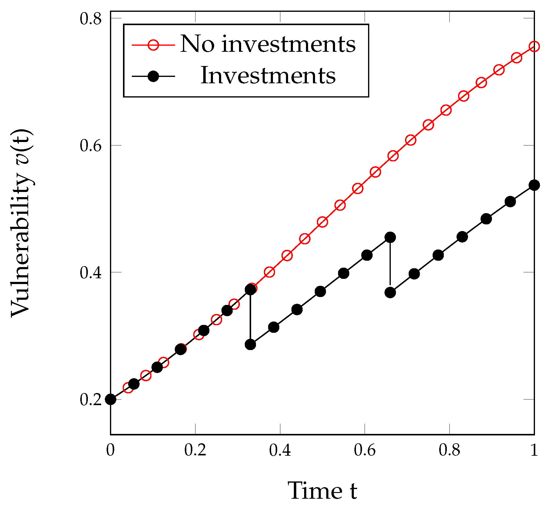
In a mixed cyber-risk management approach, the premium in the insurance component is a consequence of both exogeneous factors (the insurance company setting the base premium, and the external environment posing threats) and one’s own choices to invest. The only strategic leverages are then the amount of money to invest and when to invest. In the following we assume that investment is made periodically, so that the only choices are to set the period and the amount of money to invest. However, for the time being, we consider the impact of the investment amount only.

The straightforward goal is to minimize the overall security expense. Though this could be achieved considering the entire time horizon, for the time being, we adopt a greedy approach, where the expense minimization is conducted at each investment epoch. Our goal is then to find

$$Z_i^{*}=arg\underset{Z_i}{min}{E}_i|T,H,$$

(12)

where the investment periodicity and the overall time horizon are set, and the asterisk denotes the optimal solution.

In the following we consider all the case resulting from the combination of the liability policies (full, partial, partial with deductibles) and the investment effectiveness models (GL1 and GL2).

We start with the full liability case. In that case, we have a closed-form solution. We consider first the GL1 model. Following the derivation in [16], we zero the first derivative of the overall expense

$$\frac{\partial E_i^{\mathrm{full}}}{\partial Z_i}=1-\frac{P_{0}r\alpha \beta V}{(1+e^{-kT}(V/v_{i-1}-1)){(1+\alpha Z_i)}^{\beta +1}}=0.$$

(13)

After some passages, the resulting optimal investment is

$$Z_i^{*}=\frac{1}{\alpha }\left[{\left(\frac{P_{0}r\alpha \beta V}{1+e^{-kT}(V/v_{i-1}-1)}\right)}^{\frac{1}{\beta +1}}-1\right].$$

(14)

This extremal investment point is a sure minimum, since the second derivative is positive, being a product made of all positive factors:

$$\frac{\partial E^{\mathrm{full}}}{{\partial }_{Z_i}}=\frac{P_{0}r{\alpha }^2\beta (\beta +1)V}{(1+e^{-kT}(V/v_{i-1}-1)){(1+\alpha Z_i)}^{\beta +2}}$$

(15)

However, the straight mathematical derivation may lead us to a negative investment, which obviously makes no sense. Hence, the solution is valid if the following condition holds

$$\frac{P_{0}r\alpha \beta V}{1+e^{-kT}(V/v_{i-1}-1)}>1$$

(16)

In general, the validity is granted when

• the vulnerability $v_i$ is close to the maximum vulnerability V
• the maximum vulnerability V is large;
• the investment epochs are not too close to each other.

A similar development can be conducted when the GL2 model applies. In that case, the first derivative is

$$\frac{\partial E^{\mathrm{full}}}{{\partial }_{Z_i}}=1+P_{0}r\alpha v{\left(t_i\right)}^{\alpha Z_i+1}ln\left(v\left(t_i\right)\right)=0$$

(17)

which reaches its minimum at

$$Z_i^{*}=-\frac{1}{\alpha }\left[\frac{ln(-P_{0}r\alpha ln\left(\frac{V}{1+e^{-kT}(V/v_{i-1}-1)}\right)}{ln\left(\frac{V}{1+e^{-kT}(V/v_{i-1}-1)}\right)}+1\right].$$

(18)

The validity conditions for this expression have been thoroughly examined in [16].

We can now move to the case where the insurance company sets a ceiling for its liability. When the loss does not exceed the upper bound u, the expressions stay the same as in the full liability case. Instead, when $\lambda >u$, we obtain the following derivatives. For the GL1 model, we obtain

$$\begin{array}{cc}\hfill & \frac{\partial E_{\mathrm{i}}^{\mathrm{partial}}}{\partial Z_i}=1-\frac{P_{0}r\alpha \beta V}{(1+e^{-k(t_i-a)}){(1+\alpha Z_i)}^{\beta +1}}\hfill \\ \hfill & -\frac{V}{k}\frac{q(\lambda -u)}{T}\frac{e^{kT}-1}{V+v_i(e^{kT}-1)}\frac{V\alpha \beta }{(1+e^{kT}){(1+\alpha Z_i)}^{\beta +1}}=\hfill \\ \hfill & 1-\frac{\alpha \beta V}{(1+e^{-kT})(V/v_{i-1}-1){(1+\alpha Z_i)}^{\beta +1}}\left[P_{0}r+\frac{V}{k}\frac{q(\lambda -u)}{T}\frac{e^{kT}-1}{V+v_i(e^{kT}-1)}\right]=0\hfill \end{array}$$

(19)

For the GL2 model, we have instead

$$\begin{array}{cc}\hfill & \frac{\partial E_{\mathrm{i}}^{\mathrm{partial}}}{\partial Z_i}=1+P_{0}r\alpha {\left(\frac{V}{1+e^{-k(t_i-a)}}\right)}^{\alpha Z_i+1}ln\left(\frac{V}{1+e^{-k(t_i-a)}}\right)\hfill \\ \hfill & +\frac{V}{k}\frac{q(\lambda -u)}{t_{i+1}-t_i}\frac{\alpha (e^{kT}-1)}{V+v_i(e^{kT}-1)}{\left(\frac{V}{1+e^{-k(t_i-a)}}\right)}^{\alpha Z_i+1}ln\left(\frac{V}{1+e^{-k(t_i-a)}}\right)=\hfill \\ \hfill & 1+\alpha {\left(\frac{V}{1+e^{-kT}(V/v_{i-1}-1)}\right)}^{\alpha Z_i+1}ln\left(\frac{V}{1+e^{-kT}(V/v_{i-1}-1)}\right)\times \hfill \\ \hfill & \left[P_{0}r+\frac{V}{k}\frac{q(\lambda -u)}{T}\frac{e^{kT}-1}{V+v_i(e^{kT}-1)}\right]=0\hfill \end{array}$$

(20)

In both models, we see that the resulting equation is not amenable to a closed-form solution. In the following, we will resort to a numerical approach.

Finally, when we consider the cases where deductibles are also included in the insurance policy, we obtain the following derivatives for the expenses to minimize for the GL1 and GL2 model, respectively:

$$\begin{array}{cc}\hfill & \frac{\partial E_{\mathrm{i}}^{\mathrm{deduct}}}{\partial z_i}=1-\frac{P_{0}r\alpha \beta V}{(1+e^{-k(t_i-a)}){(1+\alpha z_i)}^{\beta +1}}\hfill \\ \hfill & -\frac{V}{k}\frac{q(\lambda -u+\ell )}{T}\frac{e^{kT}-1}{V+v_i(e^{kT}-1)}\frac{V\alpha \beta }{(1+e^{kT}){(1+\alpha z_i)}^{\beta +1}}=\hfill \\ \hfill & 1-\frac{\alpha \beta V}{(1+e^{-kT}(V/v_{i-1}-1)){(1+\alpha z_i)}^{\beta +1}}\left[P_{0}r+\frac{V}{k}\frac{q(\lambda -u+\ell )}{T}\frac{e^{kT}-1}{V+v_i(e^{kT}-1)}\right]=0\hfill \end{array}$$

(21)

$$\begin{array}{cc}\hfill & \frac{\partial E_{\mathrm{i}}^{\mathrm{deduct}}}{\partial Z_i}=1+P_{0}r\alpha {\left(\frac{V}{1+e^{-k(t_i-a)}}\right)}^{\alpha Z_i+1}ln\left(\frac{V}{1+e^{-k(t_i-a)}}\right)\hfill \\ \hfill & +\frac{V}{k}\frac{q(\lambda -u+\ell )}{t_{i+1}-t_i}\frac{\alpha (e^{kT}-1)}{V+v_i(e^{kT}-1)}{\left(\frac{V}{1+e^{-k(t_i-a)}}\right)}^{\alpha Z_i+1}ln\left(\frac{V}{1+e^{-k(t_i-a)}}\right)=\hfill \\ \hfill & 1+\alpha {\left(\frac{V}{1+e^{-kT}(V/v_{i-1}-1)}\right)}^{\alpha Z_i+1}ln\left(\frac{V}{1+e^{-kT}(V/v_{i-1}-1)}\right)\times \hfill \\ \hfill & \left[P_{0}r+\frac{V}{k}\frac{q(\lambda -u+\ell )}{T}\frac{e^{kT}-1}{V+v_i(e^{kT}-1)}\right]=0\hfill \end{array}$$

(22)

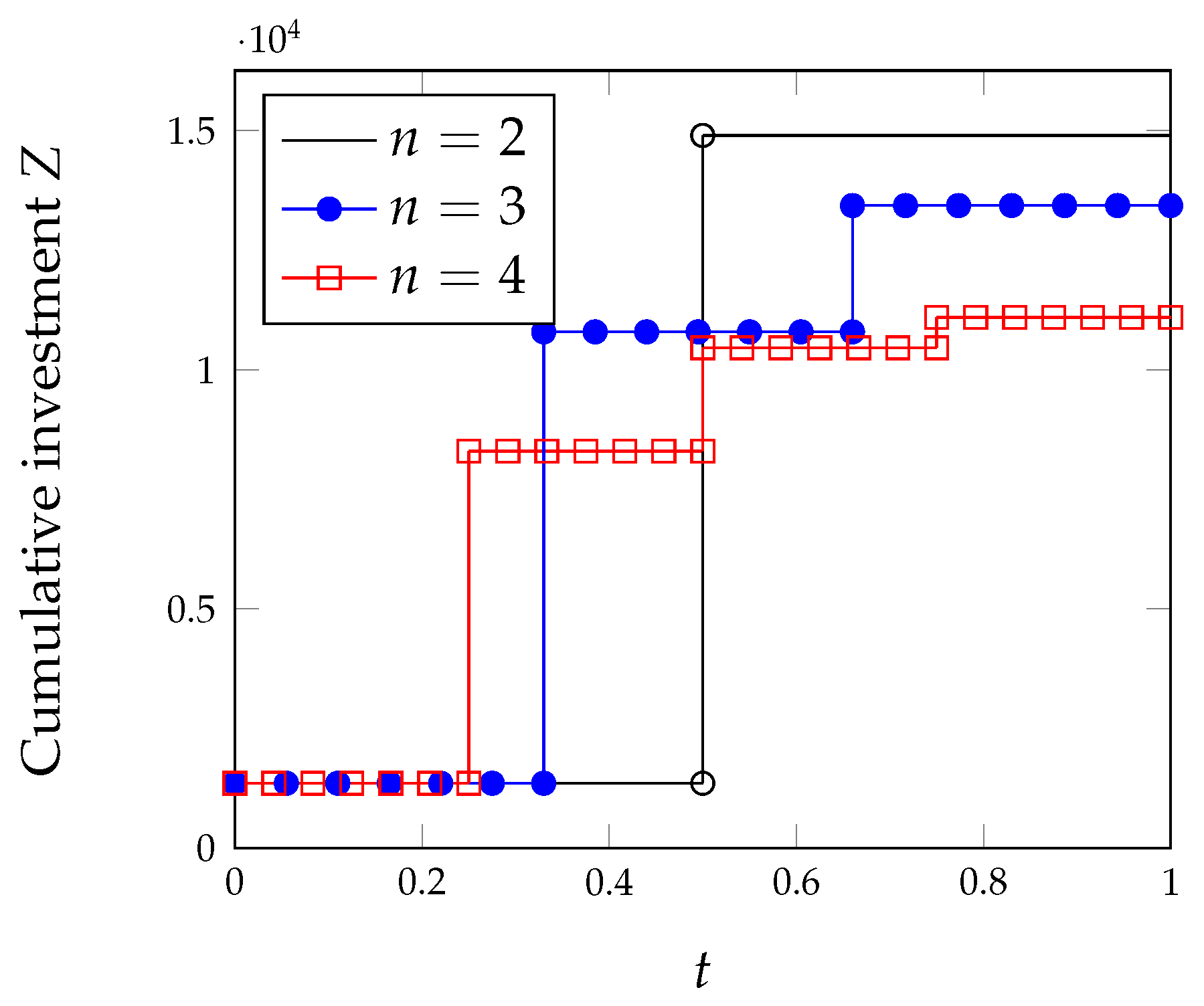
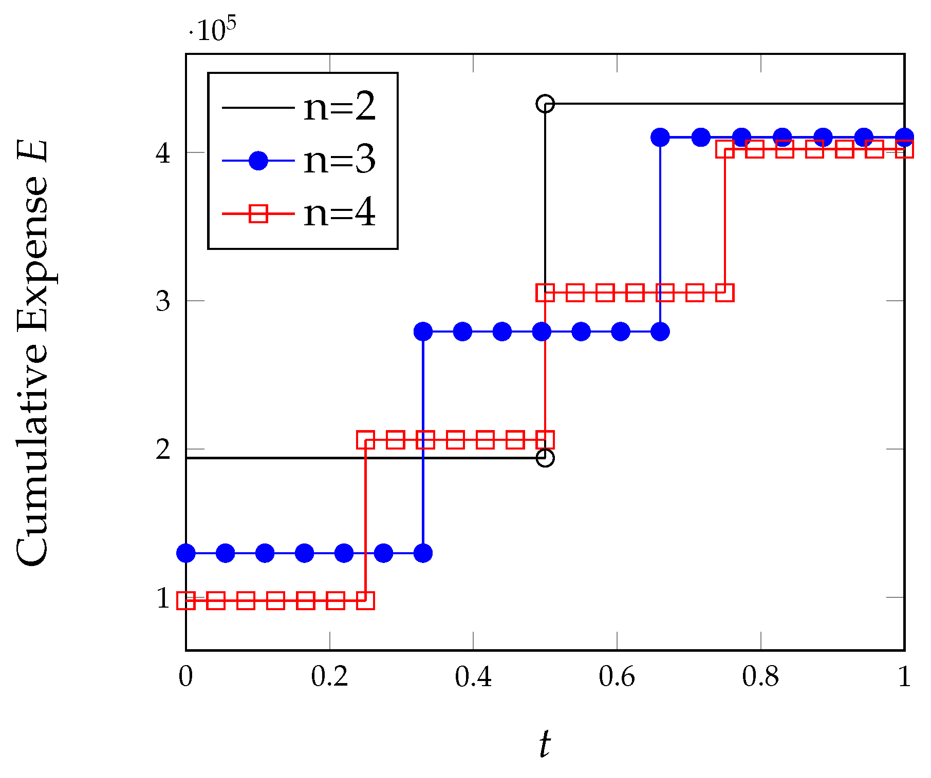
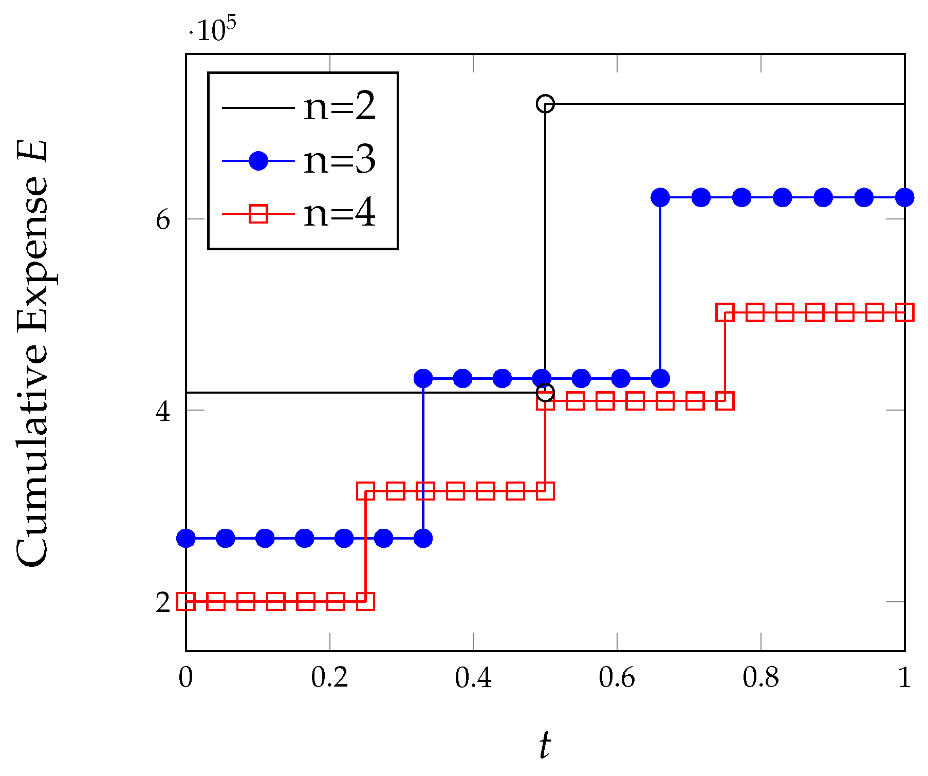
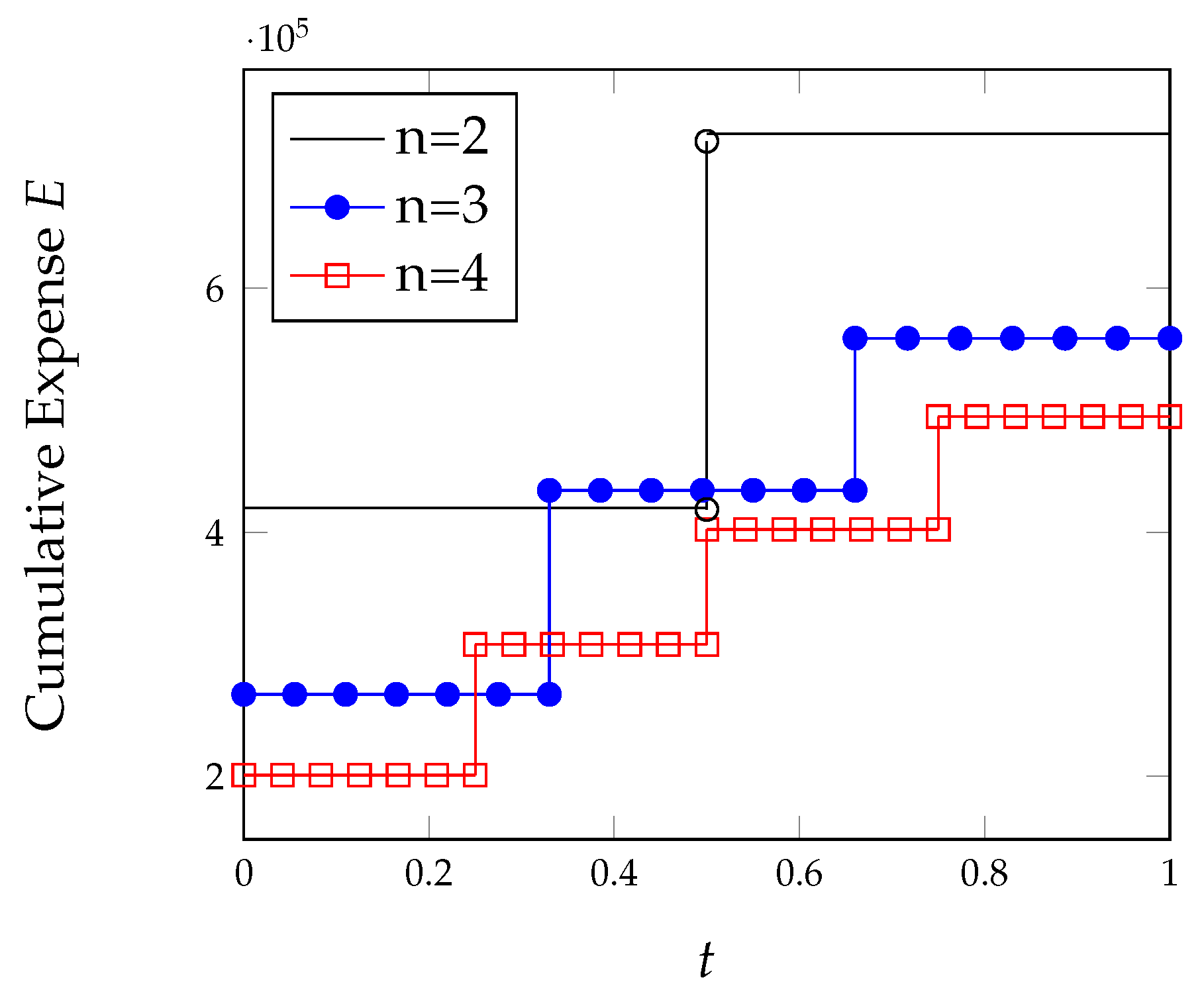
6. Example Application

After having sketched the solution to the expense minimization problem, in this section we provide some examples of its application. We are reminded that for the partial liability and the partial liability with deductible cases, we will be forced to employ a numerical approach.

In the following, we employ the values shown in

Table 1. Values of the parameters used.

Parameter	Value
$\alpha$	$2.7\times {10}^{-5}$
$\beta$	1.1
u	$8.5\times {10}^6$
ℓ	5000
$\gamma$	0.05
q	0.9
$\lambda$	${10}^7$
V	$0.95$
r	$0.5$

. We will consider a time horizon $H=1$ and $T=H/n$ with $n=2,3,4$. The premium is accordingly adjusted to take into account the duration of the insurance policy validity. In order to test different signs of the order relationship between the loss $\lambda$ and the liability thresholds ℓ and u, in the following we will consider $\lambda =5·{10}^3$ to test the case $\lambda <\ell$, $\lambda =5·{10}^6$ to test the case $\ell ,\lambda <u$, and $\lambda ={10}^7$ to test the case $\lambda >u$.

We start with the case of full liability. In Figure 2, we plot the cumulative optimal investment for the GL1 model. The initial vulnerability is $v_0=0.1$. We see that in all three periodicity cases the initial investment is zero, i.e., it is enough to rely on insurance due to the low vulnerability value. Instead, as we progress over time, breaking the overall investment into three instalments pays, since it leads to the minimum overall investment.

However, when we look at the overall expense, the picture changes just a bit. In Figure 3, we see that the best choice is still to split the investment into as many epochs as possible, though the differences among the three periodicity values flatten out at the end of the time horizon. Insurance represents the dominant component in the overall expense, being nearly an order of magnitude larger than investments.

When the insurance policy includes a partial liability, we have again a no-investment strategy for low vulnerability values, but the differences due to different periodicity values in the cumulative investment are smaller than what we saw in the full liability case, though the four-instalment solution is still the preferred choice (see Figure 4 and Figure 5). The pictures refer to the situation where the loss exceeds the liability, since no significant differences appear to the full liability case when $\lambda <u$.

When we consider the overall expenses, the dominant role of insurance is confirmed. The subdivision of investments in as many epochs as possible is also suggested.

Finally, these results are confirmed if we consider the case with deductibles, as shown in Figure 6 and Figure 7.

Similar results are found for the GL2 model. Here, we do not comment on those results, but simply show the pertaining curves in Figure 8, Figure 9, Figure 10, Figure 11, Figure 12 and Figure 13.

7. Discussion and Conclusions

We have computed the optimal mixed strategy to address a growing vulnerability over time. In all cases, the insurance component dominates by roughly an order of magnitude over investments. When the vulnerability is quite low, investments can be avoided so as to rely on insurance only. Those results appear to be valid even when the insurer’s liability reduces due to the imposition of deductibles and upper limits. The overall message is that insurance appears as the main tool to rely on in cyber-risk management, though this conclusion strongly relies on the validity of the Gordon–Loeb model to describe the effectiveness of investments. These conclusions confirm what had been found for the case of a single investment/insurance instalment with identical assumptions for the investment effectiveness (i.e., the Gordon–Loeb model) [16]. However, what emerges from the analysis in the growing vulnerability case is that a distribution of countermeasures over time (e.g., periodically re-evaluating the situation and de facto fractioning the investment/insurance) leads to a lower overall security expense. Our contribution extends the previous investigations considering the synergetic use of investments and insurance to reduce the impact of cyberattacks and is a first step to a dynamic risk-management approach. Though the time evolution of the vulnerability is described by a fixed function of time, the function parameters may be recalibrated at each time step to closely follow the actual evolution of risk.

Though these general conclusions may be expected to hold for different choices of the parameters to those employed in this paper, a limitation is represented by the greedy approach. An overall investment optimization could be applied over a longer time horizon. Additionally, while we have considered investments as the only strategic variable, we could obtain better results by allowing the timing of investments to be optimized as well, possibly considering non-uniform subdivisions of the time horizon (i.e., relaxing the periodicity constraint). In addition, the simplifying assumption of fixed losses should be replaced by the inclusion of a probability model for the severity of security breaches.

References

1. Maillart, T.; Sornette, D. Heavy-tailed distribution of cyber-risks. Eur. Phys. J. B 2010, 75, 357–364. [Google Scholar] [CrossRef]
2. Wheatley, S.; Maillart, T.; Sornette, D. The extreme risk of personal data breaches and the erosion of privacy. Eur. Phys. J. B 2016, 89, 1–12. [Google Scholar] [CrossRef] [Green Version]
3. Palsson, K.; Gudmundsson, S.; Shetty, S. Analysis of the impact of cyber events for cyber insurance. Geneva Pap. Risk Insur.-Issues Pract. 2020, 45, 564–579. [Google Scholar] [CrossRef]
4. Scala, N.M.; Reilly, A.C.; Goethals, P.L.; Cukier, M. Risk and the Five Hard Problems of Cybersecurity. Risk Anal. 2019, 39, 2119–2126. [Google Scholar] [CrossRef] [PubMed]
5. Paté-Cornell, M.E.; Kuypers, M.; Smith, M.; Keller, P. Cyber risk management for critical infrastructure: A risk analysis model and three case studies. Risk Anal. 2018, 38, 226–241. [Google Scholar] [CrossRef]
6. Refsdal, A.; Solhaug, B.; Stølen, K. Cyber-risk management. In Cyber-Risk Management; Springer: Berlin/Heidelberg, Germany, 2015; pp. 33–47. [Google Scholar]
7. Murphy, D.R.; Murphy, R.H. Teaching cybersecurity: Protecting the business environment. In Proceedings of the 2013 on InfoSecCD’13: Information Security Curriculum Development Conference, Kennesaw, GA, USA, 12 October 2013; pp. 88–93. [Google Scholar]
8. Eling, M.; McShane, M.; Nguyen, T. Cyber risk management: History and future research directions. Risk Manag. Insur. Rev. 2021, 24, 93–125. [Google Scholar] [CrossRef]
9. Biener, C.; Eling, M.; Wirfs, J.H. Insurability of cyber risk: An empirical analysis. Geneva Pap. Risk Insur.-Issues Pract. 2015, 40, 131–158. [Google Scholar] [CrossRef] [Green Version]
10. Franke, U. The cyber insurance market in Sweden. Comput. Secur. 2017, 68, 130–144. [Google Scholar] [CrossRef]
11. Xie, X.; Lee, C.; Eling, M. Cyber insurance offering and performance: An analysis of the US cyber insurance market. Geneva Pap. Risk Insur.-Issues Pract. 2020, 45, 690–736. [Google Scholar] [CrossRef]
12. Bahşi, H.; Franke, U.; Friberg, E.L. The cyber-insurance market in Norway. Inf. Comput. Secur. 2019, 28, 54–67. [Google Scholar] [CrossRef]
13. Strupczewski, G. Current state of the cyber insurance market. In Proceedings of the Economics and Finance Conferences, London, UK, 22–25 May 2018; International Institute of Social and Economic Sciences: London, UK, 2018; p. 6910062. [Google Scholar]
14. Carfora, M.F.; Martinelli, F.; Mercaldo, F. Cyber risk management: An actuarial point of view. J. Oper. Risk 2019, 14, 4. [Google Scholar]
15. Young, D.; Lopez, J.; Rice, M.; Ramsey, B.; McTasney, R. A framework for incorporating insurance in critical infrastructure cyber risk strategies. Int. J. Crit. Infrastruct. Prot. 2016, 14, 43–57. [Google Scholar] [CrossRef]
16. Mazzoccoli, A.; Naldi, M. Robustness of Optimal Investment Decisions in Mixed Insurance/Investment Cyber Risk Management. Risk Anal. 2019, 40, 550–564. [Google Scholar] [CrossRef] [PubMed]
17. Miaoui, Y.; Boudriga, N. Enterprise security economics: A self-defense versus cyber-insurance dilemma. Appl. Stoch. Model. Bus. Ind. 2019, 35, 448–478. [Google Scholar] [CrossRef]
18. Kröger, W. Critical infrastructures at risk: A need for a new conceptual approach and extended analytical tools. Reliab. Eng. Syst. Saf. 2008, 93, 1781–1787. [Google Scholar] [CrossRef]
19. Kure, H.I.; Islam, S. Assets focus risk management framework for critical infrastructure cybersecurity risk management. IET Cyber-Phys. Syst. Theory Appl. 2019, 4, 332–340. [Google Scholar] [CrossRef]
20. Gordon, L.A.; Loeb, M.P. The economics of information security investment. ACM Trans. Inf. Syst. Secur. 2002, 5, 438–457. [Google Scholar] [CrossRef]
21. Gordon, L.A.; Loeb, M.P.; Zhou, L. Investing in Cybersecurity: Insights from the Gordon-Loeb Model. J. Inf. Secur. 2016, 7, 49. [Google Scholar] [CrossRef] [Green Version]
22. Naldi, M.; Flamini, M. Calibration of the Gordon-Loeb Models for the Probability of Security Breaches. In Proceedings of the 2017 UKSim-AMSS 19th International Conference on Computer Modelling & Simulation (UKSim), Cambridge, UK, 5–7 April 2017; IEEE: Piscataway, NJ, USA, 2017; pp. 135–140. [Google Scholar]
23. Huang, C.D.; Behara, R.S. Economics of information security investment in the case of concurrent heterogeneous attacks with budget constraints. Int. J. Prod. Econ. 2013, 141, 255–268. [Google Scholar] [CrossRef]
24. Naldi, M.; Flamini, M.; D’Acquisto, G. Negligence and sanctions in information security investments in a cloud environment. Electron. Mark. 2018, 28, 39–52. [Google Scholar] [CrossRef]
25. Mayadunne, S.; Park, S. An economic model to evaluate information security investment of risk-taking small and medium enterprises. Int. J. Prod. Econ. 2016, 182, 519–530. [Google Scholar] [CrossRef]
26. Hua, J.; Bapna, S. The economic impact of cyber terrorism. J. Strateg. Inf. Syst. 2013, 22, 175–186. [Google Scholar] [CrossRef]
27. Gao, X.; Zhong, W.; Mei, S. Security investment and information sharing under an alternative security breach probability function. Inf. Syst. Front. 2015, 17, 423–438. [Google Scholar] [CrossRef]
28. Gordon, L.A.; Loeb, M.P.; Lucyshyn, W.; Zhou, L. Increasing cybersecurity investments in private sector firms. J. Cybersecur. 2015, 1, 3–17. [Google Scholar] [CrossRef] [Green Version]
29. Wu, Y.; Feng, G.; Wang, N.; Liang, H. Game of information security investment: Impact of attack types and network vulnerability. Expert Syst. Appl. 2015, 42, 6132–6146. [Google Scholar] [CrossRef]
30. Krutilla, K.; Alexeev, A.; Jardine, E.; Good, D. The Benefits and Costs of Cybersecurity Risk Reduction: A Dynamic Extension of the Gordon and Loeb Model. Risk Anal. 2021, 41, 1795–1808. [Google Scholar] [CrossRef]
31. Rosson, J.; Rice, M.; Lopez, J.; Fass, D. Incentivizing Cyber Security Investment in the Power Sector Using An Extended Cyber Insurance Framework. Homel. Secur. Aff. 2019, 15, 2. [Google Scholar]
32. Sawik, T. A linear model for optimal cybersecurity investment in Industry 4.0 supply chains. Int. J. Prod. Res. 2022, 60, 1368–1385. [Google Scholar] [CrossRef]
33. Mazzoccoli, A.; Naldi, M. Optimal Investment in Cyber-Security under Cyber Insurance for a Multi-Branch Firm. Risks 2021, 9, 24. [Google Scholar] [CrossRef]
34. Hausken, K. Returns to information security investment: The effect of alternative information security breach functions on optimal investment and sensitivity to vulnerability. Inf. Syst. Front. 2006, 8, 338–349. [Google Scholar] [CrossRef]
35. Wang, S. Optimal Level and Allocation of Cybersecurity Spending: Model and Formula. 2017. Available online: https://papers.ssrn.com/sol3/papers.cfm?abstract_id=3010029 (accessed on 15 May 2022).
36. Wang, S.S. Integrated framework for information security investment and cyber insurance. Pac.-Basin Financ. J. 2019, 57, 101173. [Google Scholar] [CrossRef]
37. Feng, S.; Xiong, Z.; Niyato, D.; Wang, P.; Wang, S.S.; Shen, X.S. Joint Pricing and Security Investment in Cloud Security Service Market with User Interdependency. IEEE Trans. Serv. Comput. 2020, 1–11. [Google Scholar] [CrossRef]
38. Jerman-Blažič, B. An economic modelling approach to information security risk management. Int. J. Inf. Manag. 2008, 28, 413–422. [Google Scholar]
39. Eling, M.; Wirfs, J. What are the actual costs of cyber risk events? Eur. J. Oper. Res. 2019, 272, 1109–1119. [Google Scholar] [CrossRef]
40. Arcuri, M.C.; Brogi, M.; Gandolfi, G. How Does Cyber Crime Affect Firms? The Effect of Information Security Breaches on Stock Returns. In Proceedings of the ITASEC, Venice, Italy, 17–20 January 2017; pp. 175–193. [Google Scholar]
41. Hovav, A.; D’Arcy, J. The impact of denial-of-service attack announcements on the market value of firms. Risk Manag. Insur. Rev. 2003, 6, 97–121. [Google Scholar] [CrossRef]
42. World Economic Forum. Partnering for Cyber Resilience: Towards the Quantification of Cyber Threats; Technical Report; World Economic Forum: Cologny, Switzerland, 2015. [Google Scholar]
43. Kamiya, S.; Kang, J.K.; Kim, J.; Milidonis, A.; Stulz, R.M. Risk management, firm reputation, and the impact of successful cyberattacks on target firms. J. Financ. Econ. 2021, 139, 719–749. [Google Scholar] [CrossRef]
44. Poufinas, T.; Vordonis, N. Pricing the Cost of Cybercrime—A Financial Protection Approach. iBusiness 2018, 10, 128. [Google Scholar] [CrossRef] [Green Version]
45. The Ponemon Institute. 2016 Cost of Data Breach Study: Global Analysis; Technical Report; The Ponemon Institute: Traverse City, MI, USA, 2016. [Google Scholar]
46. Zhuo, Y.; Solak, S. Measuring and optimizing cybersecurity investments: A quantitative portfolio approach. In Proceedings of the IIE Annual Conference, Montreal, QC, Canada, 31 May–3 June 2014; p. 1620. [Google Scholar]
47. Marotta, A.; Martinelli, F.; Nanni, S.; Orlando, A.; Yautsiukhin, A. Cyber-insurance survey. Comput. Sci. Rev. 2017, 24, 35–61. [Google Scholar] [CrossRef]
48. Kesan, J.P.; Majuca, R.P.; Yurcik, W.J. The Economic Case for Cyberinsurance; Technical Report 2; University of Illinois College of Law: Champaign, IL, USA, 2004. [Google Scholar]
49. Bolot, J.; Lelarge, M. Cyber insurance as an incentive for Internet security. In Managing Information Risk and the Economics of Security; Springer: Berlin/Heidelberg, Germany, 2009; pp. 269–290. [Google Scholar]
50. Yang, Z.; Lui, J.C. Security adoption and influence of cyber-insurance markets in heterogeneous networks. Perform. Eval. 2014, 74, 1–17. [Google Scholar] [CrossRef]
51. Pal, R.; Golubchik, L.; Psounis, K.; Hui, P. Will cyber-insurance improve network security? A market analysis. In Proceedings of the INFOCOM, 2014 Proceedings IEEE, Toronto, ON, Canada, 27 April–2 May 2014; IEEE: Piscataway, NJ, USA, 2014; pp. 235–243. [Google Scholar]
52. Shetty, N.; Schwartz, G.; Felegyhazi, M.; Walrand, J. Competitive cyber-insurance and internet security. In Economics of Information Security and Privacy; Springer: Berlin/Heidelberg, Germany, 2010; pp. 229–247. [Google Scholar]
53. Bandyopadhyay, T.; Mookerjee, V.S.; Rao, R.C. Why IT managers don’t go for cyber-insurance products. Commun. ACM 2009, 52, 68–73. [Google Scholar] [CrossRef] [Green Version]
54. Vakilinia, I.; Sengupta, S. A coalitional cyber-insurance framework for a common platform. IEEE Trans. Inf. Forensics Secur. 2018, 14, 1526–1538. [Google Scholar] [CrossRef]
55. Mukhopadhyay, A.; Chatterjee, S.; Bagchi, K.K.; Kirs, P.J.; Shukla, G.K. Cyber risk assessment and mitigation (CRAM) framework using logit and probit models for cyber insurance. Inf. Syst. Front. 2019, 21, 997–1018. [Google Scholar] [CrossRef]
56. Mazzoccoli, A.; Naldi, M. The Expected Utility Insurance Premium Principle with Fourth-Order Statistics: Does It Make a Difference? Algorithms 2020, 13, 116. [Google Scholar] [CrossRef]
57. Khalili, M.M.; Naghizadeh, P.; Liu, M. Designing cyber insurance policies: The role of pre-screening and security interdependence. IEEE Trans. Inf. Forensics Secur. 2018, 13, 2226–2239. [Google Scholar] [CrossRef]
58. Mastroeni, L.; Mazzoccoli, A.; Naldi, M. Service Level Agreement Violations in Cloud Storage: Insurance and Compensation Sustainability. Future Internet 2019, 11, 142. [Google Scholar] [CrossRef] [Green Version]
59. Herath, H.; Herath, T. Copula-based actuarial model for pricing cyber-insurance policies. Insur. Mark. Co. Anal. Actuar. Comput. 2011, 2, 7–20. [Google Scholar]
60. Meland, P.H.; Tondel, I.A.; Solhaug, B. Mitigating risk with cyberinsurance. IEEE Secur. Priv. 2015, 13, 38–43. [Google Scholar] [CrossRef]
61. Shetty, S.; McShane, M.; Zhang, L.; Kesan, J.P.; Kamhoua, C.A.; Kwiat, K.; Njilla, L.L. Reducing informational disadvantages to improve cyber risk management. Geneva Pap. Risk Insur.-Issues Pract. 2018, 43, 224–238. [Google Scholar] [CrossRef]
62. Aven, T.; Ben-Haim, Y.; Boje Andersen, H.; Cox, T.; Droguett, E.L.; Greenberg, M.; Guikema, S.; Kröger, W.; Renn, O.; Thompson, K.M.; et al. Society for Risk Analysis Glossary; Society for Risk Analysis: Herndon, VA, USA, 2018. [Google Scholar]
Figure 1. Impact of investments on vulnerability (GL1 model with α = 2.7 · 10 5 , β = 1.1 ) (logistic growth model with V = 0.95 , k = 2.68 ) (attack probability q = 0.7 ).
Algorithms 15 00211 g001
Figure 2. Optimal cumulative investment under full liability and GL1 model.
Algorithms 15 00211 g002
Figure 3. Optimal cumulative expense E under full liability and GL1 model.
Algorithms 15 00211 g003
Figure 4. Optimal cumulative investment under partial liability and GL1 model.
Algorithms 15 00211 g004
Figure 5. Optimal cumulative expense E under partial liability and GL1 model.
Algorithms 15 00211 g005
Figure 6. Optimal cumulative investment under partial liability with deductibles and GL1 model.
Algorithms 15 00211 g006
Figure 7. Optimal cumulative expense E under partial liability with deductibles and GL1 model.
Algorithms 15 00211 g007
Figure 8. Optimal cumulative investment under full liability and GL2 model.
Algorithms 15 00211 g008
Figure 9. Optimal cumulative expense E under full liability and GL2 model.
Algorithms 15 00211 g009
Figure 10. Optimal cumulative investment under partial liability and GL2 model.
Algorithms 15 00211 g010
Figure 11. Optimal cumulative expense E under partial liability and GL2 model.
Algorithms 15 00211 g011
Figure 12. Optimal cumulative investment under partial liability with deductibles and GL2 model.
Algorithms 15 00211 g012
Figure 13. Optimal cumulative Expense E under partial liability with deductibles and GL2 model.
Algorithms 15 00211 g013