Gravity-Law Based Critical Bots Identification in Large-Scale Heterogeneous Bot Infection Network

Abstract

The explosive growth of botnets has posed an unprecedented potent threat to the internet. It calls for more efficient ways to screen influential bots, and thus precisely bring the whole botnet down beforehand. In this paper, we propose a gravity-based critical bots identification scheme to assess the influence of bots in a large-scale botnet infection. Specifically, we first model the propagation of the botnet as a Heterogeneous Bot Infection Network (HBIN). An improved SEIR model is embedded into HBIN to extract both heterogeneous spatial and temporal dependencies. Within built-up HBIN, we elaborate a gravity-based influential bots identification algorithm where intrinsic influence and infection diffusion influence are specifically designed to disclose significant bots traits. Experimental results based on large-scale sample collections from the implemented prototype system demonstrate the promising performance of our scheme, comparing it with other state-of-the-art baselines.

1. Introduction

Botnets have posed an unprecedented potent threat to the internet due to the explosive growth of IoT (Internet of Things) devices in recent years [1]. The core of a botnet is to exploit the vulnerabilities existing in the current vast number of IoT devices and to monetize infected devices through illicit activities on peer-to-peer (P2P) models. Representative botnets, including Mirai and Mozi [2], are able to launch a spree of massive distributed denial-of-service (DDoS) attacks with overwhelming traffic sourced from a large number of powerful devices. Traditional host-based defense measures, e.g., anti-viruses (AVs), are struggling to keep pace with the increasing sophistication of botnets. It calls for effective surveillance techniques to obtain insight into the entire situation of a large-scale botnet before it takes shape.

As a response to this persistent yet rapidly evolving botnet threat, hundreds of scientific works have investigated botnet properties within various approaches. Simple Susceptible-Exposed-Infectious-Removed (SEIR) models combined with Markov chain have been widely adopted to measure the total infected population [3]. However, as summarised in [4], these works concentrate more on revealing the propagation property while overlooking the global topology information of the botnet. From a typical governance point of view, it is important to explore a botnet’s vulnerability, i.e., identify those crucial bots whose corruptions bring the whole botnet work down to its knees.

There have also been a substantial number of works proposing different approaches to account for botnet governance [5,6,7,8,9,10]. Unfortunately, these approaches do not seem to represent the entire spatial-temporal characteristics together with the heterogeneity of botnets. Since botnet infection is typically a complex activity with propagation behaviors to observe, it is unclear whether current complex work solutions can indeed automatically learn the representation of botnet infection and thereby output valid prediction results. In addition to deficient patterns, none of these works verified their models in the real world. Consequently, they are far less likely to be readily applied to alleviate the spread of botnets.

To comprehensively tackle a large-scale botnet infection problem fundamentally, two crucial questions are raised naturally. The first one is how to devise a feasible model to depict both local and global topology dependencies among bots, as well as portray the significant propagation pattern across heterogeneous spatial-temporal dimensions, and verify its effectiveness in the real world. The second challenge lies in how to design an effective method that is capable of precisely disclosing multiple significant botnet infection characteristics. Thus it can comprehensively weigh the influence of botnet nodes in heterogeneous spatial-temporal dimensions for key bots identification.

Jointly considering the challenges above, in this paper, we propose a novel critical bot identification scheme, to explore the influential bots in a large-scale botnet infection. We model the propagation of a botnet as a Heterogeneous Bot Infection Network (HBIN) to extract both heterogeneous spatial and temporal dependencies, where an improved SEIR model is embedded to deeply reveal the transition states of bot devices during infection. Based on the built HBIN, we distinguish the influences of bots among the HBIN into diffusion influences and intrinsic influences, which respectively focus on global topology compromise and bots’ interactions with neighbours. We further present a Gravity-law based Critical Bots Identification (GCBI) algorithm where intrinsic influence and infection diffusion score are specifically designed to disclose significant bots’ influential traits.

In a nutshell, our major contributions are summarized as follows:

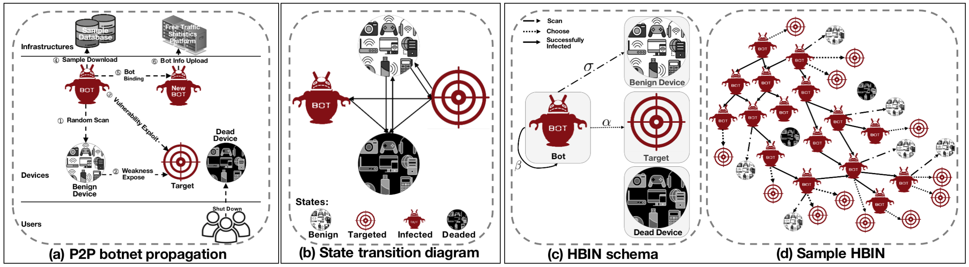
• We elaborate a SEIR-based HBIN by utilizing the advantages of the SEIR model and a heterogeneous information network (HIN), where the SEIR model depicts the transition states of bots, and HIN provides the heterogeneous spatial-temporal dependencies among various botnet devices. Such a comprehensive HBIN is capable of representing significant propagation characteristics on a global bot infection network for further influential bots identification;
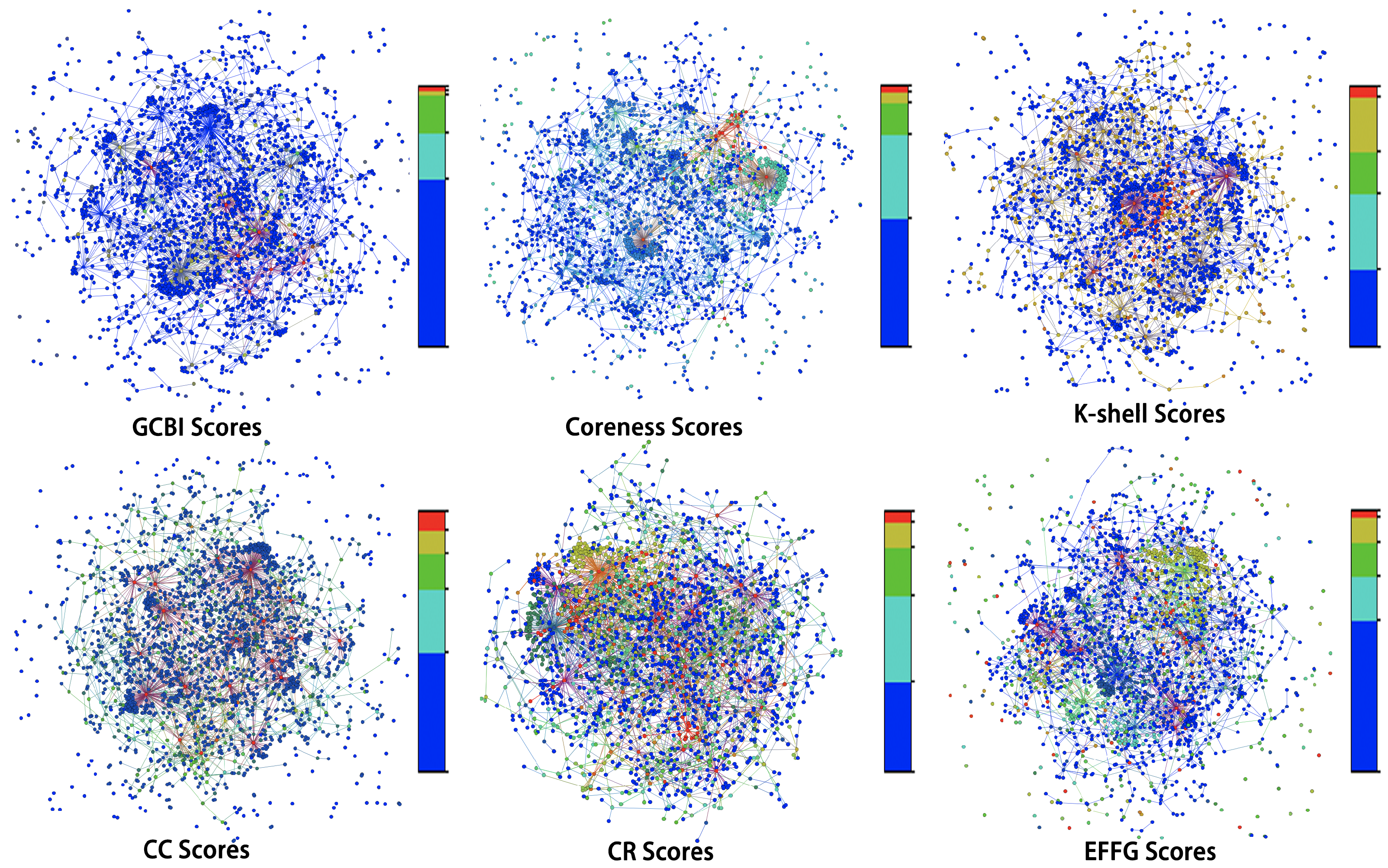
• We design a Gravity-law based Critical Bots Identification algorithm based on HBIN, which distinguishes the influences of bots into intrinsic influences and diffusion influences. Such a GCBI algorithm is capable of identifying the critical bots in both local and global potential structural heterogeneous temporal-spatial dimensions;
• We implement an IoT botnet monitor system and collect millions of bot samples with distinct labels. We evaluate the effectiveness of our proposed algorithm with extensive experiments on the large-scale real dataset.

The remainder of this paper is organized as follows: Section 2 introduces our constructed model for depicting botnet infection. Section 3 presents the details of the critical bot identification scheme. Section 4 provides a discussion on the results gained from the extensive experiments. Section 5 shows system deployment and impacts. In Section 6, we review some related work. Finally, Section 7 draws final conclusions.

2. Botnet Infection Model

In this section, we first briefly introduce the propagation process of a botnet and next present a SEIR-based HBIN model to characterize botnet propagation pattern. To better understand the botnet propagation, we take Mozi botnet as a typical example to provide a summary of a botnet’s operation gleaned from our botnet tracing system. As indicated in Figure 1a, building a large-scale epidemic botnet network heavily relies on exploiting weakness recursively. The workflow of the botnet propagation is illustrated as follows: (1) Target scanning: At the start of the infection, a bot node scans for benign devices by choosing IP addresses randomly; (2) Weakness discovery: Susceptible devices with weak credentials will be labeled as the targets; (3) Vulnerability exploiting: The bot node attempts to exploit vulnerabilities at a target and then plants a malicious sample into the target device if it exploits it successfully; (4) Bot binding: Once the target has been infected, the bot node binds the victim to the related port and tries to connect to peer nodes; (5) Botnet forming: During the propagation of a botnet, more and more benign nodes would be targeted by old bots and turned into newly recruited bots recursively. Based on how P2P communication takes place, the botnet forms an overlay topology.

On the other hand, the devices may die sporadically due to the failure of the network or system. However, if the dead node is resurrected, it is also able to be recruited by the botnet.

2.1. SEIR State Transition Diagram

Since botnet propagation is similar to disease transmission in a population, we can depict the transition states of bots by employing the SEIR epidemic model.

As indicated in Figure 1b, there are four entity types in botnet propagation, i.e., Benign, Target, Bot, Dead. For an individual node, it can be affected and transformed into other types under certain conditions. For instance, initial ‘Benign’ nodes would be marked as ‘Targeted’ nodes when they encounter vulnerability exploitation, and ‘Targeted’ entities would also be turned into ‘Infected’ if a bot loads a malicious sample into them successfully. In other words, each individual node could possess different states during botnet propagation. The entire individual node’s transition state diagram formally also consists of four distinct states—Benign(B), Targeted(T), Infected(I) and Dead(D), which correspond to Susceptible(S), Exposed(E), Infected(I) and Recovered(R) in the SEIR model, respectively. Benign(B) refers to the state where a vulnerable device has not been infected. Targeted(T) denotes the state where a device with potential weakness has been found by other bot nodes but is temporarily unable to infect others. Infected(I) indicates a device that has been infected by the other bots and can spread pestilences to others with a certain probability. The Dead(D) state denotes the quarantined or healed entity thus permanently immune to the current pestilences.

The detailed notations of transition states and corresponding conditions are summarised in

Table 1. The explanation of state transform diagram. Note that the transitions we pay more attention to are in bold.

Transition	Conditions
$\mathbf{B}\to \mathbf{T}$	Become the target of a bot
$B\to D$	Device is closed, or vulnerabilities are repaired
$T\to B$	Vulnerabilities exploiting failed
$\mathbf{T}\to \mathbf{I}$	Vulnerabilities exploiting is successful
$T\to D$	Device is closed, or vulnerabilities are patched
$I\to D$	Device is closed, or vulnerabilities are patched
$D\to B$	Device is opened, or new vulnerability are emerged

. According to the analysis of the botnet propagation process, we can verify that two transition state pairs, i.e., Benign(B) to Targeted(T), and Targeted(T) to Infected(I), play an important role in the expansion of a botnet. In what follows, we build a heterogeneous botnet infection network to investigate the dynamic characteristic of botnet infection mainly based on these two transition state pairs.

2.2. HBIN Model

We next build a Heterogeneous Bot Infection Network (HBIN) that is capable of modeling the heterogeneous spatial-temporal dependencies in botnet infection.

In the context of botnet infection, the HBIN can be defined as a weighted heterogeneous graph $G=(\mathcal{V},\mathcal{E},\mathcal{O},\mathcal{R},\mathcal{W})$, where $\mathcal{V}$ is the set of vertices representing multiple IoT device nodes, $\mathcal{E}$ is the set of multiple directed edges representing the relations among multiple nodes. $\mathcal{O}$ and $\mathcal{R}$ represent the set of node types and that of spatial-temporal edge types, respectively. Note that each node in $\mathcal{V}$ is attributed to a type, e.g., $Benign\left(B\right)$ or $Bot\left(O\right)$, depending on its current state in botnet infection. Meanwhile, every edge in $\mathcal{E}$ is associated with a unique directed label from $\mathcal{R}$ illustrating a spatial-temporal relation between two nodes, e.g., a $Bot$ node chooses one specific $Target\left(T\right)$ to launch infection action, such as vulnerability exploitation. Obviously, we have $\left|\mathcal{O}\right|+\left|\mathcal{R}\right|\ge 3$ for a heterogeneous network. Each edge in $\mathcal{E}$ is also assigned a weight in $\mathcal{W}$ according to its edge type, which represents the occurrence probability of different relations, e.g., the probability that a $Bot$ node chooses one specific $Target\left(T\right)$ to launch infection action. As a result, a graph G with various types of nodes equipped with weights on different edges is called a Heterogeneous Bot Infection Network. To accelerate the modeling of HBIN, we provide two type mapping functions in practice, i.e., $\varphi :\mathcal{V}\to \mathcal{O}$ and $\phi :\mathcal{E}\to \mathcal{R}$, to retrieve the type of a given node, as well as the type of a given edge, respectively.

Before the entire botnet data can be loaded into the HBIN G, we abstract an infection schema graph for G, which can be considered a “dictionary” of HBIN G. The infection schema defines the types of vertices and edges in the graph and how those types of vertices are related to one another. Formally, as shown in Figure 1c, the schema graph of HBIN can be denoted as ${\mathcal{T}}_G=(\mathcal{O},\mathcal{R},\mathcal{W})$ with node types, edge types and edge weights from G.

Based on the analysis of the SEIR state transform diagram above, we formally define a HBIN schema with four node types, denoted as $\mathcal{O}=\left\{Benign\right(B)$, $Target\left(T\right)$, $Bot\left(O\right)$, $Dead\left(D\right)\}$. We also define three important types of relations, that is, edges among nodes that have a great impact on botnet propagation, which are denoted as $\mathcal{R}=\left\{Scan\right(S)$, $Choose\left(C\right)$, $SuccessfullyInfected\left(SI\right)\}$. In this HBIN schema, $Scan\left(S\right)$ refers to the relation that a Bot(O) node scans its neighboring Benign(B) devices; $Choose\left(C\right)$ denotes that a $Bot$ node chooses one specific $Target\left(T\right)$ to launch infection action; while $SuccessfullyInfected\left(SI\right)$ indicates the relation whereby a $Bot\left(O\right)$ successfully infected a certain new $Bot\left(O\right)$. We use $\mathcal{W}=\{\sigma$, $\alpha$, $\beta \}$ to denote the weights of three corresponding edges $\mathcal{R}=\left\{Scan\right(S)$, $Choose\left(C\right)$, $SuccessfullyInfected\left(SI\right)\}$, indicating the occurrence probability of edge-represented relations, respectively. Specifically, $\sigma$ describes the occurrence probability that a $Bot\left(O\right)$ scans its neighboring $Benign\left(B\right)$ devices. $\alpha$ indicates the probability that a $Bot$ node chooses a $Target\left(T\right)$ to launch an infecting action, such as vulnerability exploiting. The $\alpha$ value depends largely on the node’s attributes itself, including ip-type, location and available ports since these attributes are always bound to some specific vulnerabilities. We define the formula of $\alpha$ as follows:

$$\alpha ={\alpha }_1·x_1+{\alpha }_2·x_2+b,$$

(1)

where $0<\alpha <1$, ${\alpha }_1$ and ${\alpha }_2$ are coefficients that are associated with ip-type and location of device respectively. $x_1$ and $x_2$ are numerical values respectively representing ip-type and location for a specific device. b is the bias coefficient. Note that ${\alpha }_1$, ${\alpha }_2$, b are pre-learned via NN-1, which is a neural network with one neuron. In NN-1, it inputs the feature vectors which synthetically represent attributes of a specific node, and outputs the “1” or “0”, where “1” indicates that the device is easily the target of botnet infection, and vice versa.

More specifically, the edge weight $\beta$ refers to the occurrence probability that a $Bot$ successfully infects a certain new $Bot\left(O\right)$. Intuitively, its value is determined by two continuous steps. The first step is that a $Bot\left(O\right)$ locks a $Target\left(T\right)$ and is ready to launch an infecting action whose occurrence possibility is indicated by weights $\alpha$. The following step describes the process that a $Bot\left(O\right)$ converts the $Target\left(T\right)$ to a new $Bot\left(O\right)$ successfully. Mathematically, $\beta$ can be calculated by the following formula:   

$$\beta =\alpha ·\frac{N_I}{N_T},$$

(2)

where $N_T$ and $N_I$ are the total number of Targeted devices and Infected devices in the botnet. $\frac{N_I}{N_T}$ is the fixed probability from global statistics.

According to the analysis above, each dynamic node infection event can be represented as a quad $e=(v_i,r,w,v_j)$ where $v_i$ and $v_j$ are source and target nodes, $r\in \mathcal{R}$ is the event type, and $w\in \mathcal{W}$ refers to the event occurrence probability. For example, $v_i$ denotes a $Bot\left(O\right)$, $v_j$ refers to a $Target\left(T\right)$, then r denotes a $Choose\left(C\right)$ relation representing a fact that $v_i$ chooses one specific $v_j$ to launch infecting action with a probability $w=\alpha$.

The HBIN schema provides heterogeneous spatial-temporal dependencies among infected bot nodes during botnet infection through infecting diffusion paths. As such, we can characterize a botnet dynamic diffusion path of bot infection as $Bot\left(O\right)\stackrel{SI\left(\beta \right)}{\to }Bot\left(O\right)\stackrel{SI\left(\beta \right)}{\to }Bot\left(O\right)$. This dynamic diffusion path is a semantic abstraction that illustrates a dynamic infecting process that a bot continuously conscripts new indirect bots through the directly infected bots with a certain probability $\beta$.

Given the proposed HBIN schema, we detail the process of HBIN generation in Algorithm 1. The initial network includes massive $Benign$ devices, a few $Bot$s and $Dead$ devices. The basic idea of Algorithm 1 is to extend the bot-conscripted network by infecting new devices iteratively. The generation process halts until the botnet is immune to infection, i.e., most $Benign$ devices become $Bot$s.

Algorithm 1: Heterogeneous Bot Infection Network Generation Algorithm.

3. Critical Bots Identification

To explore the most influential bots in HBIN, we first analyze the characteristics of bots infection based on real botnet traces from 3 to 27 August 2021 with the capability of CNCERT’s Global IoT botnet monitoring system. We draw a HBIN that represents the infecting interactions among bots. As shown in Figure 2, the darker the bots, the larger propagating ability they have, which implies two important facts. Firstly, bots with higher infection influence would have more domination over the network, because more infections are propagated through those bots. Secondly, highly infectious bots have more compact infection links with the other highly infectious bots, which indicates that a bot with large contagion is likely to attract the other influential bots. In other words, a bot with multiple infectious edges has higher impacts on nearby nodes and thus is likely to be more influential, which is similar to the properties of representative gravity law.

Inspired by these observations, we present a Gravity-law based Critical Bots Identification (GCBI) scheme based on the built HBIN. The rough idea of GCBI scheme takes into account both neighborhood bots’ interaction and diffusion information, where a bot with larger infection degrees (neighborhood interaction) and averagely shorter infection distances to other bots (diffusion information) is more influential.

Formally, given a HBIN $G=(\mathcal{V},\mathcal{E},\mathcal{O},\mathcal{R},\mathcal{W})$ and an integer M, GCBI scheme aims to find the M maximum allowed number of bots $I_G=\{I{D}_1,I{D}_2,I{D}_3,\dots ,I{D}_m\}$ that should be singled out for special treatment. To better compromise topological and neighborhood information in the infection process, we distinguish the influences of bots among the HBIN into intrinsic influences and diffusion influences, which capture the interacting capability with other neighbors and diffusion capability in topology, respectively. As a result, the actual infectious influences of a bot in HBIN can be estimated as a weighted sum of its neighborhood intrinsic influences and diffusion influence. Specifically, for a bot $u\in \mathcal{E}$ with bot $v\in \mathcal{E}$ as its neighbor, the true infecting influences of bot u, i.e., $TI{I}_u$, can be mathematically represented as follows:

$$TI{I}_u=S_{ii}\left(u\right)+\sum _{v\in N_{out}\left(u\right)}{w}_r\left(v\right)S_{ii}\left(v\right),$$

(3)

where $S_{ii}\left(u\right)$ and $S_{ii}\left(v\right)$ are intrinsic influences for bot u and v, respectively. $w_r\left(v\right)=\frac{weight(u,v)}{{\sum }_{j\in N_{out}\left(u\right)}weight(u,j)}$, which denotes the ratio of edge weight $E_{uv}$ to total out edge weights for bot u. Note that $weight(u,v)$ indicates the probability of infection from bot u to another bot v, we have $weight(u,v)=\beta$, which can be calculated by Equation (2). Equation (3) indicates that the correlations between a bot and its neighbors, i.e., the true infecting influence of a bot depend on the intrinsic influences of itself and the neighbors it infects (diffusion influences) directly.

Intrinsic Influence Calculation We next investigate the calculation of intrinsic influence. Naturally, a bot node with multiple infection links is more likely to be influential. On the other hand, it has higher impacts on nearby nodes and fewer impacts on the bots far from it. Based on above issues, we leverage the gravity law to evaluate the intrinsic influence of the bot, which can be represented as follows:

$$S_{ii}\left(u\right)=S_{id}\left(u\right)\sum _{v\ne u}\frac{outdeg\left(v\right)}{D{(u,v)}^2},$$

(4)

where $S_{id}\left(u\right)$ is a diffusion score of bot u that is used to measure the diffusion influences of bots, i.e., its impacts on nearby nodes. $outdeg\left(v\right)$ is the number of infection edges sourced from bot v. $D(u,v)$ denotes the effective infection distance from u to v. According to Equation (4), we can verify that a node with many infected neighbors and close to the most influential nodes will derive a larger intrinsic influence in HBIN. To further investigate the diffusion influence of bots, we will explain effective infection distance $D(u,v)$ and diffusion score $S_{id}\left(u\right)$ in detail in what follows.

Effective infection distance $D(u,v)$. In the context of HBIN, we define effective infection distance to assess how many hops there are apart from two bots along the infection path. We already know that the edge weight of HBIN indicates the probability of infection from one bot u to another v, i.e., $weight(u,v)=\beta$, effective infection distance highlights the shortest route that infects throughout two bots. To describe the distances between two bots in a network with precision, we formulate $D(u,v)$ as follows:

$$D(u,v)=min\{1-lo{g}_2\left(P{(u,v)}^{*}\right)\},$$

(5)

where $P{(u,v)}^{*}$ denotes the probability of u to choose its direct or indirect downstream attainable neighbor v, $P{(u,v)}^{*}$ is formulated as follows:

$$P{(u,v)}^{*}=P(u,l_1)\times P(l_1,l_2)\times ...\times P(l_{n-1},l_n)\times P(l_n,v),$$

(6)

where $P(l_i,l_{i+1})$ is the probability of $l_i$ choosing its direct neighbor $l_{i+1}$, which is defined as follows:

$$P(l_i,l_{i+1})=\frac{weight(l_i,l_{i+1})}{outdeg\left(l_i\right)},$$

(7)

where $\frac{1}{outdeg\left(l_i\right)}$ denotes the average probability of choosing $l_{i+1}$ from many direct neighbors of $l_i$, $weight(l_i,l_{i+1})$ indicates the occurrence probability of the infection event from $l_i$ to $l_{i+1}$. Note that $P(l_i,l_j)\ne P(l_j,l_i)$, and $P(l_i,l_i)=0$; we can verify that $D(l_i,l_i)$ is also infinite.

Diffusion Influence Calculation. We employ infection diffusion score $S_{id}\left(u\right)$ to measure the diffusion influence of bots by globally sorting bots into different levels of shells. Different levels of shells are analogous to houses labeled with different levels of index, where bot nodes are respectively placed according to their infectious ability. The bots in the innermost shell have the highest infectious capacity while bots in the outermost shell have the smallest. To calculate the non-negative infectious capacity of bots, we propose a decomposition scheme to place bots into different levels of shells and therefore derive the final infection diffusion score for an individual bot.

The decomposition scheme can be considered as an iteration process. In each iteration, each bot in HBIN calculates its infection diffusion score. If its score is lower than the current index of the assigned house, the bot will be pruned. With the iterative decomposition process, the bots possessing the most infectious ability will be pruned at the last round.

Note that the infection diffusion score in the decomposition process concentrates more on the edges where the bot infects the other bots (out-degree) instead of the bots infected (in-degree). For ease of presentation, we use exhausted out-degree $k_{out}^e(·)$ to denote the removed neighbor bots number, and $N_{out}^e$ to denote the removed neighbor bots during each decomposition iteration. Similarly, residual out-degree $k_{out}^r(·)$ indicates the remaining neighbor bots number and $N_{out}^r$ indicates the remaining neighbor bots. Mathematically, the diffusion influence for a given bot can be represented as an infection diffusion score:

$$S_{id}\left(u\right)=\lambda k_{out}^r+(1-\lambda )\sum _{v\in N_{out}^r\left(u\right)}weight(u,v)+\eta \left(\lambda k_{out}^e+(1-\lambda )\sum _{v\in N_{out}^e\left(u\right)}weight(u,v)\right),$$

(8)

where $\lambda$, $\eta$ are tunable coefficients between 0 and 1, which are used to adjust the impact ratio of different factors to infectious influence. After generating the infection diffusion scores for all bots, bots are clustered into different levels of shells by a $S_{id}$ controlled iterative decomposition process. All bots in a shell ($SID$-shell) have the same $S_{id}$ value. The higher the $S_{id}$ value is, the greater the bot diffusion influence is. We present the detailed procedure of bot infection diffusion score calculation in HBIN in Algorithm 2.

Algorithm 2: Infection diffusion score calculation.

4. Implementation and Evaluations

In this section, we conduct a series of experiments to evaluate the feasibility and performance of our proposed GCBI scheme.

4.1. Experiment Setup

Experiments were implemented under the Windows 10 operating system, equipped with a Ryzen 5600X processor, AMD, California, America, two NVIDIA GTX960 graphics cards and 16 GB of RAM. Our DHIN model was developed with Python 3.6.0.

Data Acquisition and Preparation. To derive the large-scale raw botnet data, we implemented a prototype system to collect the samples of botnet activities with a distinct timestamp and interaction label automatically. The sources of botnet samples can roughly be divided into two categories: one is generated by active probing, the other is derived from traffic analysis. We deployed an active probing system where a probe module was integrated to look for the active bots. As malicious attackers often execute an HTTP request to exploit IoT nodes, we also employed a traffic analysis approach by collecting a vast number of real botnet exploiting traces from the Internet from 3 to 27 August 2021 with the capability of CNCERT’s Global IoT botnet monitor system. Tens of thousands of botnet nodes together with their interactions were extracted from the collected botnet samples.

To better emulate the real infection phenomena on HBIN, we employed the SI epidemic model [11] to be the benchmark. Note that each botnet node has its different $\beta$ value (i.e., the probability of infected) calculated by Equation (2) in our SI simulation. We only paid attention to the epidemic spreading ability of bots, i.e., ’susceptible’ state and ’infection’ state regardless of ’dead’ state. Because we believe that dead nodes will not affect the weighting of bots’ effective infection influence and the infection trend globally.

The key parameter Settings and Network attributes of the experiment are summarized in

Table 2. Network attributes of HBIN constructed by the dealt data used in the experiments.

Dataset	N	${\mathit{T}}_{\mathit{N}}$	${\mathit{N}}_{\mathit{O}}$	${\mathit{N}}_{\mathit{T}}$	${\mathit{N}}_{\mathit{B}}$	${\mathit{N}}_{\mathit{D}}$	E	${\mathit{T}}_{\mathit{E}}$	${\mathit{E}}_{\mathit{S}}$	${\mathit{E}}_{\mathit{C}}$	${\mathit{E}}_{\mathit{SI}}$	${\mathit{d}}_{\mathit{out}}$	ND	${\mathit{p}}_{\mathit{mean}}$	C
HBIN	18,611	4	12,810	5689	100	12	14,473	3	500	13,737	236	1.072	14	3.082	0.00003

.

Where the attributes’ interpretation are:

• Nodes count (N);
• Node types count ($T_N$);
• $Bot$ nodes number ($N_O$);
• $Target$ nodes number ($N_T$);
• $Benign$ nodes number ($N_B$);
• $Dead$ nodes number ($N_D$);
• Edges count (E);
• Edge types count ($T_E$);
• $Scan$ edge number ($N_S$);
• $Choose$ edge number ($N_I$);
• $Successfullyinfected$ edge number ($N_{SI}$);
• The average of node out-degree ($d_{out}$);
• Network diameter ($ND$): largest value of the shortest path distance between any two nodes;
• The average of shortest path length ($p_{mean}$): the average of shortest path length between any two nodes;
• The average of clustering coefficient (C): the average local clustering coefficient over all the nodes;

4.2. Baseline Methods and Metrics

In this experiment, our numerical studies were based on the comparisons with several state-of-the-art baseline algorithms, which can be roughly classified into two groups: local solution and global solution. Note that local solution refers to the algorithms that only take their neighbors’ information into consideration for critical node identification, i.e., Degree centrality (DC) [12], LocalRank [12] and Neighborhood coreness [13]. Global solution includes K-shell [14], M-shell [15], Clossness centrality (CC) [16], Betweenness centrality (BC) [17], PageRank [18], ClusterRank [19], GM [20] and EFFG [21], which are capable of utilizing the global structure information of network to quantify nodes’ importance.

All baseline algorithms were implemented in Python. Each baseline algorithm would generate a critical bots list. Without losing generality, we leveraged Kendall’s $\tau$ value [22] and monotonicity [13] as the metrics to assess the correctness of the generated bots list. Kendall’s $\tau$ value is a standard approach to compare two ranked lists, which is formulated as follows:

$$\tau =\frac{2}{N(N-1)}\sum _{i<j}sgn\left[(x_i-x_j)(y_i-y_j)\right],$$

(9)

where $sgn\left(x\right)$ is a sign function, N denotes the total number of nodes in the ranking lists, and $x_i$, $x_j$ and $y_i$, $y_j$ are the order values in the two ranking lists for the nodes i and j respectively.

Monotonicity is a measure of the uniqueness of rank value assigned to each node. We employed monotonicity to understand the effectiveness and the quality of the ranking list generated by different methods, which is formally expressed as:

$$M\left(R\right)={\left[1-\frac{{\sum }_{r\in R}{n}_r(n_r-1)}{N(N-1)}\right]}^2,$$

(10)

where $n_r$ is the total number of those nodes with the same rank r, and N is the total number of the nodes in the ranking list R.

4.3. Performance Comparison

We first studied the comparison of GCBI algorithm with the other baseline algorithms by investigating infection influence. As shown in Figure 3, we drew a heat map to illustrate the distribution of the bots’ importance. In the right color scale card, the proportion of different colors indicates the proportion of bots number in different influence score scales. Note that the darker the bot color is, the more highly influential the bot is. We can observe that the heat map generated by GCBI is well discriminated by red (higher influence) and blue (lower influence) colors. On the contrary, the other baselines have to employ more colors to describe their importance distribution. These observations imply that the proposed GCBI algorithm is able to distinguish critical bots more accurately compared with the other baselines.

We next investigated the impact of different algorithms on identifying influential bot nodes in HBIN. We applied the SI [23] model on our HBIN networks. Note that each botnet node has its different $\beta$ value (i.e., the probability of infected) calculated by Equation (2) in our SI simulation. The top-10 bot nodes generated by six different methods were first selected. We then set the top-10 bot nodes as the initial infectious bots in the SI model separately. Note that we ran the SI simulation experiment 1000 times independently for each method. We calculated the average of total bots number, directly or indirectly, infected by the set of 10 initial infectious bots up to time T respectively. The bots that generated more infected nodes up to time T are more influential. The results are shown in Figure 4. The steeper the curve is, the more influential the 10 bots in the initial infectious set are. It can be seen that our proposed GCBI algorithm denoted by the dark blue curve derives the best performance compared with the other algorithms. The bots number infected by 10 infectious bot nodes generated by our GCBI is about 15% higher than the second best baseline algorithm, i.e., ClusterRank (CR), which is identified by the light blue curve. This result practically demonstrates the effectiveness of our proposed method for critical bots identification.

To further investigate the effectiveness of our GCBI algorithm, we conducted extensive experiments by running eleven baseline methods in our constructed HBIN. Each baseline method generates a ranking list with top-5 critical bots. We applied Kendall’s $\tau$ values and the monotonicity values of GCBI to compare their relative performance in identifying critical bots. The detail of performance comparisons is shown in

Table 3. Comparison with baseline methods.

	SI	GCBI	DC	Coreness	k-Shell	m-Shell	CC	BC	PR	CR	GM	EFFG	Greedy
Top-5 ranking of crucial bots in HBIN selected by our proposed method, other state-of-the-art methods and SI benchmark model
1	231	231	95	95	3025	201	95	95	87	231	87	231	9665
2	226	226	87	87	1551	212	87	87	2271	226	212	226	951
3	229	229	2271	2271	229	9665	10,380	1980	95	229	49	229	3320
4	212	212	523	65	226	11,159	11,626	1698	11,626	201	5635	200	7
5	70	228	65	523	228	1753	96	1695	5989	200	8969	212	7377
The total number of the same bots between SI benchmark method and other methods for the ranked top-5 bots
Sum	5	4	0	0	1	0	0	0	0	3	0	3	0
Kendall’s $\tau$ values and the monotonicity values of our proposed method along with other state-of-the-art methods
$\tau$	1	0.556	0.156	0.244	0.067	0.111	−0.067	0.032	−0.111	0.2	−0.022	0.333	0.114
M	1	0.928	1	0.054	0.277	0.99	0.195	1	1	0.898	1	0.419	1

. We can observe that the top-5 overlapping number generated by GCBI algorithm is 4, while $\tau$ is about 0.556, which are both the largest compared with the other global algorithms. This result confirms that the proposed GCBI algorithm is more effective than the benchmarks. The rationale is that the proposed GCBI can successively explore dynamic infection interactions along the diffusion path. We also notice that the monotonicity values M of GCBI algorithm are close to 1. In contrast, the benchmarks, i.e., coreness, k-shell, Closeness Centrality, and EFFG result in relatively low monotonicity values. This phenomenon indicates that GCBI can attain the most critical bot node set with efficiency and high quality since it fully and specifically considers various significant and influential botnet infection features across multiple dimensions instead of just considering a certain feature in a certain dimension. Obviously, GCBI is practical for precisely selecting critical bots in a large-scale bot infection network.

5. System Deployment and Impacts

By adopting the proposed scheme, our GCBI algorithm has already been incorporated into CNCERT’s Global IoT Botnet Monitor System for over 12 months. The Botnet Monitor System is able to deal with super-large-scale infection networks and effectively finds critical influential bot nodes for different botnets within the response time threshold. It collects about 100,000 newly found IoT Bot nodes per week and distinguishes about $1\%$ key bots from millions of nodes. CNCERT has demonstrated its performance at quickly identifying critical bots. In the short run, the system will be deployed in the anti-botnet industry to provide surveillance services against botnet rampant expansion.

6. Related Work

Extensive works have investigated botnet properties within various approaches. However, the literatures that are closely related to this paper roughly fall into three categories: botnet analysing, epidemic modeling and key nodes identification.

With the rapid expansion of botnets, many works focus on understanding, detecting and mitigating botnets. The remarkable research of Antonakakis et al. [24] studied the rapid rise of Mirai and its subversion of the fragile IoT ecosystem through a 7-month retrospective analysis of the number of infected hosts and DDos victims to disclose some significant characteristics, such as the time of appearance, fragile devices it targeted and infected, the attacks it carried out and the modes of propagation. Along this line, the botnet characteristics obtained by analysis are further widely utilized for detection [25]. Generally, the majority of existing detection approaches [25,26,27,28,29,30,31] focus on particular botnet C&C (command and control) protocols and network structures, e.g., centralized or P2P, flow and graph based features.

The application of epidemic modeling originated in the medical field to study disease incidence among people [8]. Due to its effectiveness at modeling propagation behavior, there exists a large number of works that apply it to modeling vulnerability [4,7,8,10,32,33]. Kephart et al. [34] first introduced the epidemic model to cyber-security with the study of modeling computer viruses. In [7], Lu et al. used the SI (Susceptible-Infected) model to construct a semi-distributed P2P Botnet growth model that extends the classical worm propagation SEM model. Along this line, Antonakakis et al. [4] designed a state-based model to observe botnet propagation with mobile actuators. Recently, more stochastic versions of these epidemic models tend to use Markov Processes or stochastic differentials. In [35], Abaid et al. leveraged Markov chain to build a botnet propagation and infection model, helping to predict botnet attacks and provide early warnings to network administrators. As summarised in [10], epidemic modeling is capable of explaining the discrepancy in botnet propagation well. However, they overlooked global topology information and failed to represent the entire spatial-temporal characteristics together with the heterogeneity of the botnet. Our work adopts the SIER model to keep the dynamic properties of botnet infection while leveraging HIN to represent topological characteristics, as it has shown efficiency in complex topology portraying [36].

In recent years, critical nodes identification [20,21,37,38,39,40,41,42] has been widely studied in complex networks. Typical identification methods include abstract distance [21], information entropy (IE) [38,39,40,41,42,43] and machine learning [29]. Shang et al. [21] introduced effective distance to replace the Euclidean Distance for identifying influential nodes based on information fusion and multi-level processing. Liu et al. [37] proposed a generalized weighted gravity model, called the Generalized Mechanical Model (GMM), which is capable of considering both local information based on neighbors and global information based on paths in both directed and undirected networks. Note that most of the existing works mainly concentrate on spatial characteristics, and it is unclear whether existing key nodes identification can indeed comprehensively consider the significant characteristics of botnet infection and thereby output critical bots precisely.

Differing from these works, our work leverages advances of epidemic modeling and key nodes identification techniques, which are capable of disclosing the significant propagation characteristics of botnet infection across spatial-temporal dimensions for finding critical bots with the most influence that contribute significantly to zombie pestilence diffusion.

7. Conclusions

IoT botnets have been a painful problem for the internet. In this paper, we studied the problem of critical nodes identification in vast botnet infection. We modeled the propagation of a botnet as a HBIN integrated with SEIR to disclose significant infection features. Based on a heterogeneous bot infection network, we proposed a Gravity-law based Critical Bots Identification scheme to assess the influence of botnet nodes. The proposed critical bots identification scheme, mixed with intrinsic influence and infection diffusion influence, is capable of measuring the influence of a botnet node by considering various significant traits in HBIN. Experimental results demonstrate the effectiveness of our proposed scheme compared with the state-of-the-art methods based on a large-scale real-world dataset.

References

1. Trautman, L.J.; Hussein, M.T.; Ngamassi, L.; Molesky, M.J. Governance of the Internet of Things (loT). Jurimetrics J. 2020, 60, 315–351. [Google Scholar]
2. Xu, Y.; Jiang, Y.; Yu, L.; Li, J. Brief Industry Paper: Catching IoT Malware in the Wild Using HoneyIoT. In Proceedings of the IEEE 27th Real-Time and Embedded Technology and Applications Symposium (RTAS), Nashville, TN, USA, 18–21 May 2021; pp. 433–436. [Google Scholar]
3. Evesti, A.; Kanstrén, T.; Frantti, T. Cybersecurity situational awareness taxonomy. In Proceedings of the 2017 International Conference on Cyber Situational Awareness, Data Analytics and Assessment (Cyber SA), London, UK, 19–20 June 2017; pp. 1–8. [Google Scholar]
4. Antonakakis, M.; April, T.; Bailey, M.; Bernhard, M.; Bursztein, E.; Cochran, J.; Durumeric, Z.; Halderman, J.A.; Invernizzi, L.; Kallitsis, M.; et al. Understanding the mirai botnet. In Proceedings of the 26th USENIX Security Symposium (USENIX Security 17), Vancouver, BC, Canada, 16–18 August 2017; pp. 1093–1110. [Google Scholar]
5. Xie, J.; Tan, L. Fake-honeypot Detection Method for Semi-distributed Peer-to-Peer Botnet. Jisuanji Gongcheng/Comput. Eng. 2010, 36, 111–113. [Google Scholar]
6. Schiller, C.; Binkley, J.R. Botnets: The killer Web Applications; Elsevier: Amsterdam, The Netherlands, 2011. [Google Scholar]
7. Lu, Z.; Wang, W.; Wang, C. On the evolution and impact of mobile botnets in wireless networks. IEEE Trans. Mob. Comput. 2015, 15, 2304–2316. [Google Scholar] [CrossRef]
8. Kolias, C.; Kambourakis, G.; Stavrou, A.; Voas, J. DDoS in the IoT: Mirai and other botnets. Computer 2017, 50, 80–84. [Google Scholar] [CrossRef]
9. Systems and Networks Research Lab. Available online: https://sysnet.lums.edu.pk/ (accessed on 2 May 2016).
10. Al-Sarawi, S.; Anbar, M.; Alieyan, K.; Alzubaidi, M. Internet of Things (IoT) communication protocols. In Proceedings of the 2017 8th International Conference on Information Technology (ICIT), Amman, Jordan, 17–18 May 2017; pp. 685–690. [Google Scholar]
11. Pastor-Satorras, R.; Vespignani, A. Epidemic spreading in scale-free networks. Phys. Rev. Lett. 2001, 86, 3200. [Google Scholar] [CrossRef] [PubMed] [Green Version]
12. Chen, D.; Lü, L.; Shang, M.S.; Zhang, Y.C.; Zhou, T. Identifying influential nodes in complex networks. Phys. A Stat. Mech. Its Appl. 2012, 391, 1777–1787. [Google Scholar] [CrossRef] [Green Version]
13. Bae, J.; Kim, S. Identifying and ranking influential spreaders in complex networks by neighborhood coreness. Phys. A Stat. Mech. Its Appl. 2014, 395, 549–559. [Google Scholar] [CrossRef]
14. Kitsak, M.; Gallos, L.K.; Havlin, S.; Liljeros, F.; Muchnik, L.; Stanley, H.E.; Makse, H.A. Identification of influential spreaders in complex networks. Nat. Phys. 2010, 6, 888–893. [Google Scholar] [CrossRef] [Green Version]
15. Zeng, A.; Zhang, C.J. Ranking spreaders by decomposing complex networks. Phys. Lett. A 2013, 377, 1031–1035. [Google Scholar] [CrossRef] [Green Version]
16. Sabidussi, G. The centrality index of a graph. Psychometrika 1966, 31, 581–603. [Google Scholar] [CrossRef]
17. Wang, W.; Tang, M.; Stanley, H.E.; Braunstein, L.A. Unification of theoretical approaches for epidemic spreading on complex networks. Rep. Prog. Phys. 2017, 80, 036603. [Google Scholar] [CrossRef] [PubMed]
18. Page, L.; Brin, S.; Motwani, R.; Winograd, T. The PageRank Citation Ranking: Bringing Order to the Web; Technical Report; Stanford InfoLab: Stanford, CA, USA, 1999. [Google Scholar]
19. Chen, D.B.; Gao, H.; Lü, L.; Zhou, T. Identifying influential nodes in large-scale directed networks: The role of clustering. PLoS ONE 2013, 8, e77455. [Google Scholar] [CrossRef] [PubMed] [Green Version]
20. Ma, L.l.; Ma, C.; Zhang, H.F.; Wang, B.H. Identifying influential spreaders in complex networks based on gravity formula. Phys. A Stat. Mech. Its Appl. 2016, 451, 205–212. [Google Scholar] [CrossRef] [Green Version]
21. Xie, Y.; Wang, X.; Jiang, D.; Xu, R. High-performance community detection in social networks using a deep transitive autoencoder. Inf. Sci. 2019, 493, 75–90. [Google Scholar] [CrossRef]
22. Knight, W.R. A computer method for calculating Kendall’s tau with ungrouped data. J. Am. Stat. Assoc. 1966, 61, 436–439. [Google Scholar] [CrossRef]
23. Shang, Q.; Deng, Y.; Cheong, K.H. Identifying influential nodes in complex networks: Effective distance gravity model. Inf. Sci. 2021, 577, 162–179. [Google Scholar] [CrossRef]
24. Team Cymru. Available online: http://www.team-cymru.org/ (accessed on 23 January 2022).
25. Abou Daya, A.; Salahuddin, M.A.; Limam, N.; Boutaba, R. A graph-based machine learning approach for bot detection. In Proceedings of the 2019 IFIP/IEEE Symposium on Integrated Network and Service Management (IM), Arlington, VA, USA, 8–12 April 2019; pp. 144–152. [Google Scholar]
26. Alieyan, K.; ALmomani, A.; Manasrah, A.; Kadhum, M.M. A survey of botnet detection based on DNS. Neural Comput. Appl. 2017, 28, 1541–1558. [Google Scholar] [CrossRef]
27. Pektaş, A.; Acarman, T. Botnet detection based on network flow summary and deep learning. Int. J. Netw. Manag. 2018, 28, e2039. [Google Scholar] [CrossRef]
28. Pektaş, A.; Acarman, T. Effective feature selection for botnet detection based on network flow analysis. In Proceedings of the International Conference Automatics and Informatics, Madrid, Spain, 26–28 July 2017; pp. 1–4. [Google Scholar]
29. Stevanovic, M.; Pedersen, J.M. On the use of machine learning for identifying botnet network traffic. J. Cyber Secur. Mobil. 2016, 4, 32. [Google Scholar] [CrossRef] [Green Version]
30. Dua, S.; Du, X. Data Mining and Machine Learning in Cybersecurity; CRC Press: Boca Raton, FL, USA, 2016. [Google Scholar]
31. Chowdhury, S.; Khanzadeh, M.; Akula, R.; Zhang, F.; Zhang, S.; Medal, H.; Marufuzzaman, M.; Bian, L. Botnet detection using graph-based feature clustering. J. Big Data 2017, 4, 1–23. [Google Scholar] [CrossRef] [Green Version]
32. Kong, X.; Li, N.; Zhang, C.; Shen, G.; Ning, Z.; Qiu, T. Multi-Feature Representation based COVID-19 Risk Stage Evaluation with Transfer Learning. IEEE Trans. Netw. Sci. Eng. 2022, 9, 1359–1375. [Google Scholar] [CrossRef]
33. Xia, F.; Wang, L.; Tang, T.; Chen, X.; Kong, X.; Oatley, G.; King, I. CenGCN: Centralized Convolutional Networks with Vertex Imbalance for Scale-Free Graphs. IEEE Trans. Knowl. Data Eng. 2022. [Google Scholar] [CrossRef]
34. Kephart, J.O.; White, S.R. Directed-graph epidemiological models of computer viruses. In Computation: The Micro and the Macro View; World Scientific: Singapore, 1992; pp. 71–102. [Google Scholar]
35. Abaid, Z.; Sarkar, D.; Kaafar, M.A.; Jha, S. The early bird gets the botnet: A markov chain based early warning system for botnet attacks. In Proceedings of the 2016 IEEE 41st Conference on Local Computer Networks (LCN), Dubai, United Arab Emirates, 7–10 November 2016; pp. 61–68. [Google Scholar]
36. Hasan, M.K.; Ismail, A.F.; Islam, S.; Hashim, W.; Ahmed, M.M.; Memon, I. A novel HGBBDSA-CTI approach for subcarrier allocation in heterogeneous network. Telecommun. Syst. 2019, 70, 245–262. [Google Scholar] [CrossRef]
37. Liu, F.; Wang, Z.; Deng, Y. GMM: A generalized mechanics model for identifying the importance of nodes in complex networks. Knowl.-Based Syst. 2020, 193, 105464. [Google Scholar] [CrossRef]
38. Hu, P.; Mei, T. Ranking influential nodes in complex networks with structural holes. Phys. A Stat. Mech. Its Appl. 2018, 490, 624–631. [Google Scholar] [CrossRef]
39. Wang, Z.; Du, C.; Fan, J.; Xing, Y. Ranking influential nodes in social networks based on node position and neighborhood. Neurocomputing 2017, 260, 466–477. [Google Scholar] [CrossRef]
40. Zareie, A.; Sheikhahmadi, A.; Fatemi, A. Influential nodes ranking in complex networks: An entropy-based approach. Chaos Solitons Fractals 2017, 104, 485–494. [Google Scholar] [CrossRef]
41. Wang, M.; Li, W.; Guo, Y.; Peng, X.; Li, Y. Identifying influential spreaders in complex networks based on improved k-shell method. Phys. A Stat. Mech. Its Appl. 2020, 554, 124229. [Google Scholar] [CrossRef]
42. Da Silva, L.N.; Malacarne, A.; e Silva, J.W.S.; Kirst, F.V.; De-Bortoli, R. The Scientific Collaboration Networks in University Management in Brazil. Creat. Educ. 2018, 9, 1469. [Google Scholar] [CrossRef] [Green Version]
43. Shetty, J.; Adibi, J. Discovering important nodes through graph entropy the case of enron email database. In Proceedings of the 3rd International Workshop on Link Discovery, Chicago, IL, USA, 21–24 August 2005; pp. 74–81. [Google Scholar]
44. HBIN. Available online: https://github.com/w0xing/HBIN_data (accessed on 23 January 2022).
Figure 1. Botnet Infection Model.
Electronics 11 01771 g001
Figure 2. A sample of infection graph.
Electronics 11 01771 g002
Figure 3. The heat map of different methods calculated influence scores in HBIN. Note that the proportion of different colors in the right color scale card indicates the proportion of nodes number in different influence score segments.
Electronics 11 01771 g003
Figure 4. The figure compares the infection ability of the top-10 bot nodes selected by different methods in HBIN.
Electronics 11 01771 g004