Studying Disease Reinfection Rates, Vaccine Efficacy, and the Timing of Vaccine Rollout in the Context of Infectious Diseases: A COVID-19 Case Study


Abstract
1. Introduction
Motivation for Model Comparison
2. The Compartmental Models
- Emigration and birth are excluded due to the closure of the international airport and a blockade during the study period, preventing immigration and emigration. Those entering during this time underwent a 10-day quarantine.
- Individuals in the infected (symptomatic) compartment are quarantined, minimizing interactions with the susceptible population, except for caregivers who contract the disease separately.
- Vaccination is targeted towards exposed individuals who recover, while those who have already been infected and recovered do not receive the vaccine, having developed antibodies.
- Susceptible ( and S), exposed, and recovered individuals are vaccinated at the same rate.
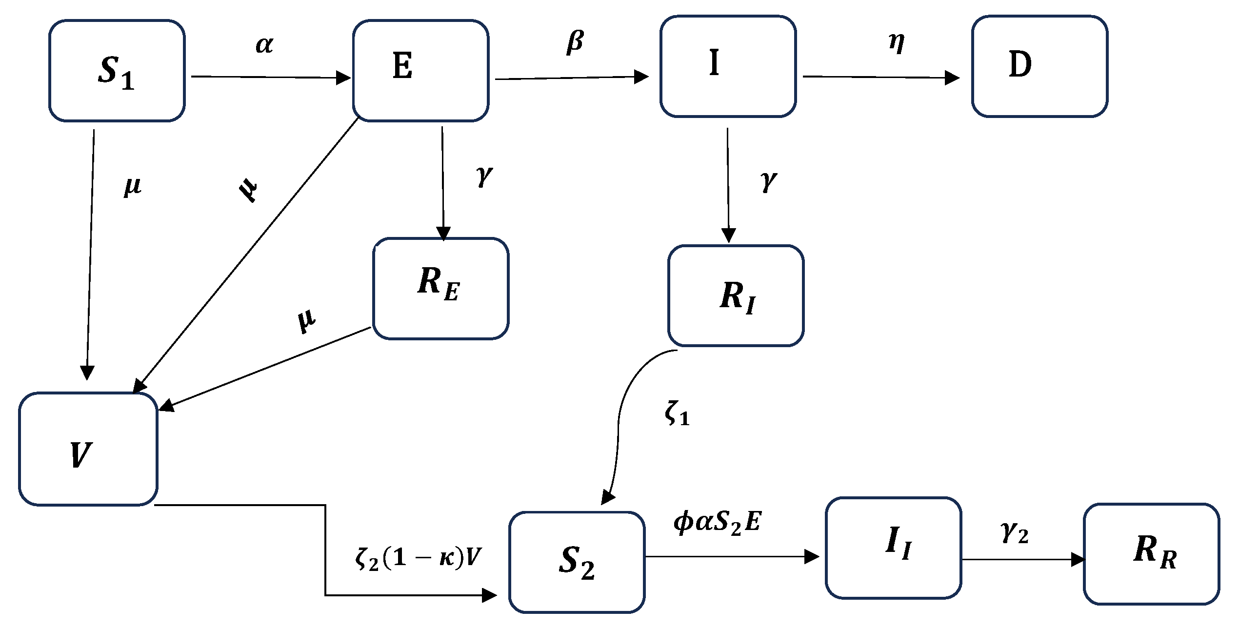
2.1. The EIRDV Model
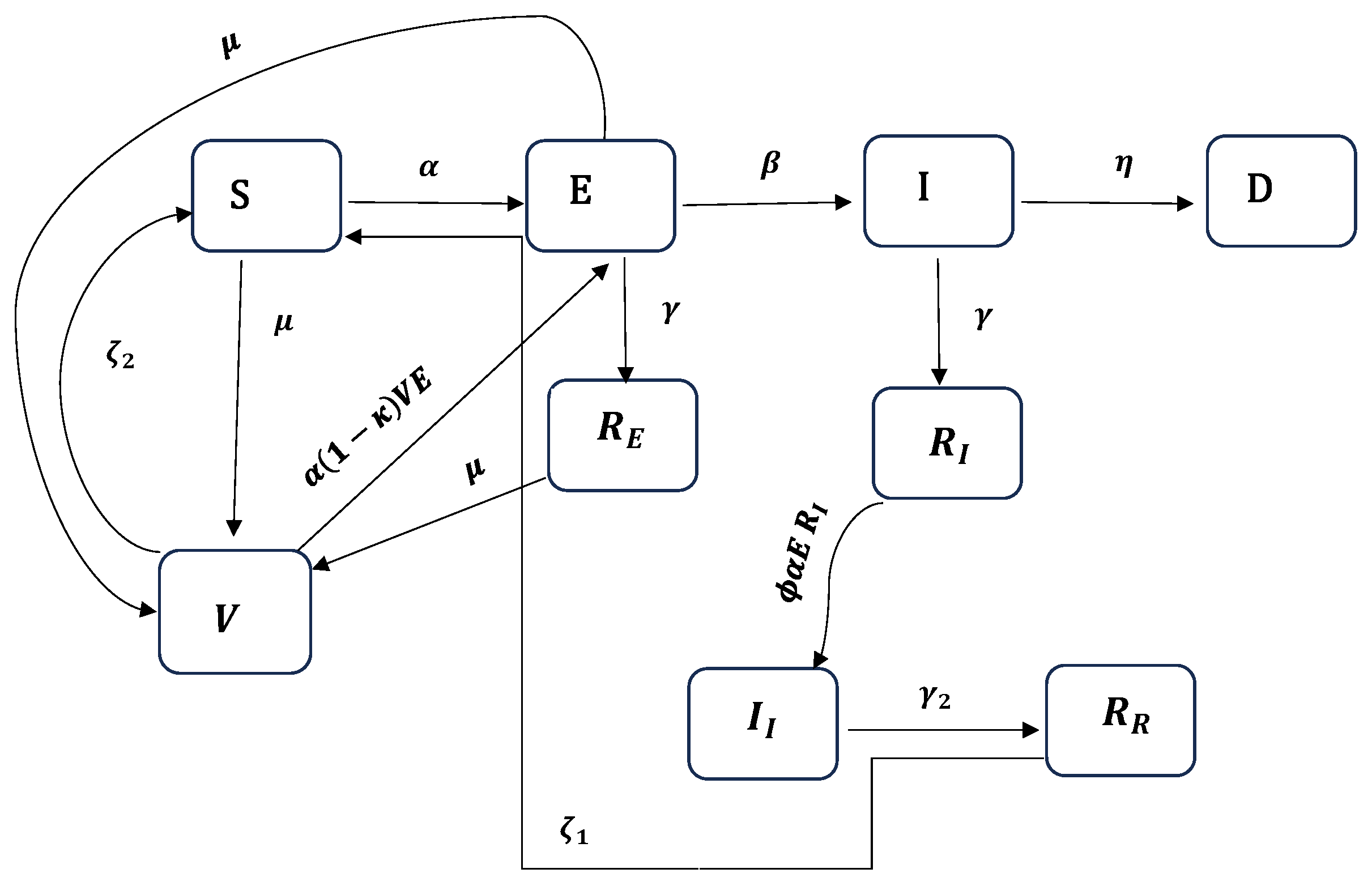
2.2. The SEIRDV Model
3. Statistical Methodology for Model Inference and Model Comparison
3.1. The Bayesian Analysis Framework
3.2. Bayesian Model Comparison Using Bayes Factor
3.3. Assessing ‘Closeness’ of Density Plots Using Hellinger Distance
4. Results
4.1. Scenario Analyses of Vaccine Efficacy and Timing of Hospital Overload Using Models 1 and 2
4.2. Hellinger Distance Analysis
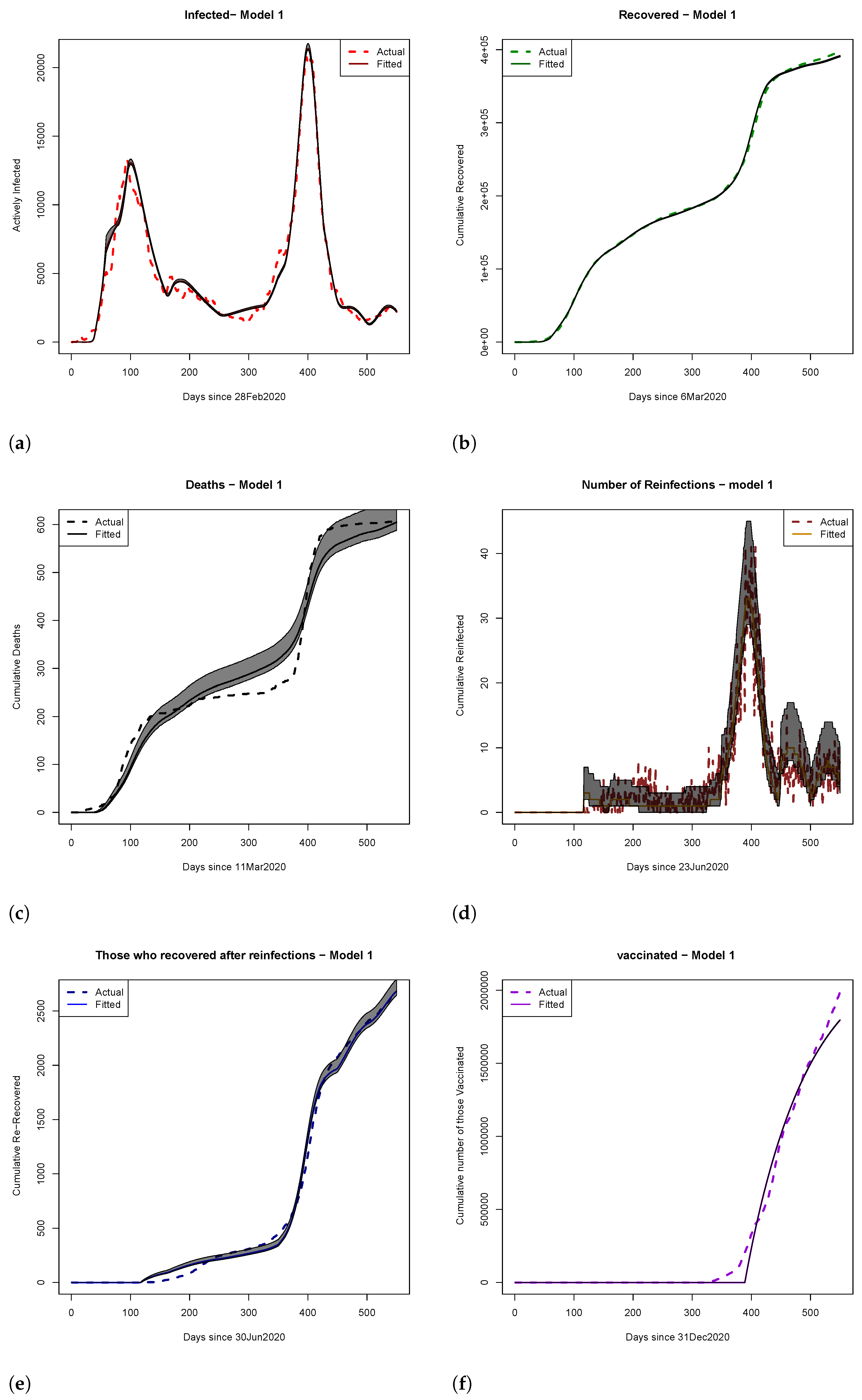
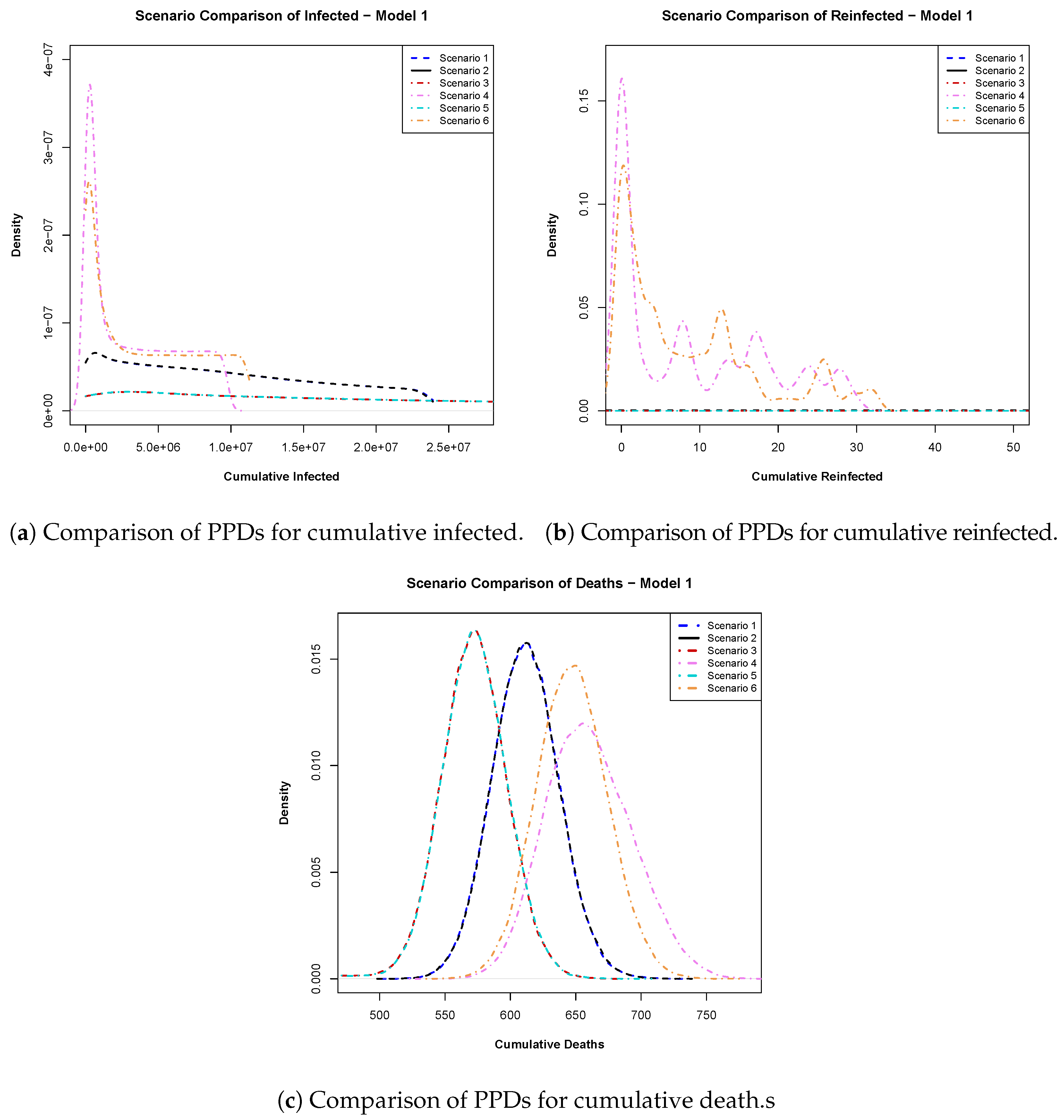
- Model 1: In Figure 5a, we analyzed the posterior predictive distributions for cumulative infections calculated for day 540 within a 550-day time frame. Scenarios involving a 94% efficacious vaccine (scenario 1) and a 100% efficacious vaccine (scenario 2) exhibited high similarity, suggesting that pursuing an ideal vaccine did not significantly affect case control. Conversely, scenarios 1 and 3 (early vaccine with 94% efficacy) displayed substantial dissimilarity, emphasizing the impact of vaccination timing. Late vaccinations (scenarios 4 and 6) showed a preference for 100% vaccine efficacy over 94%.
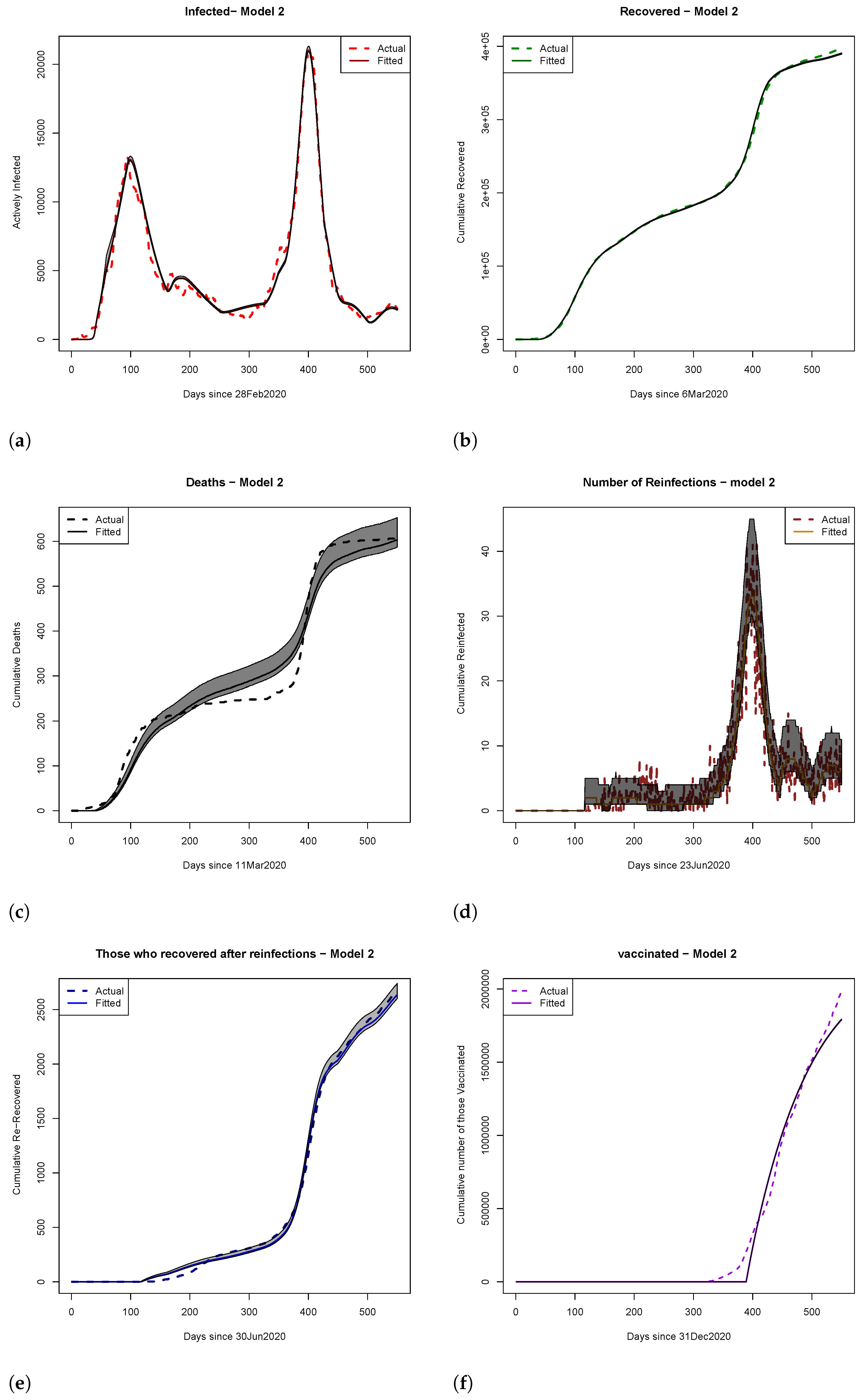
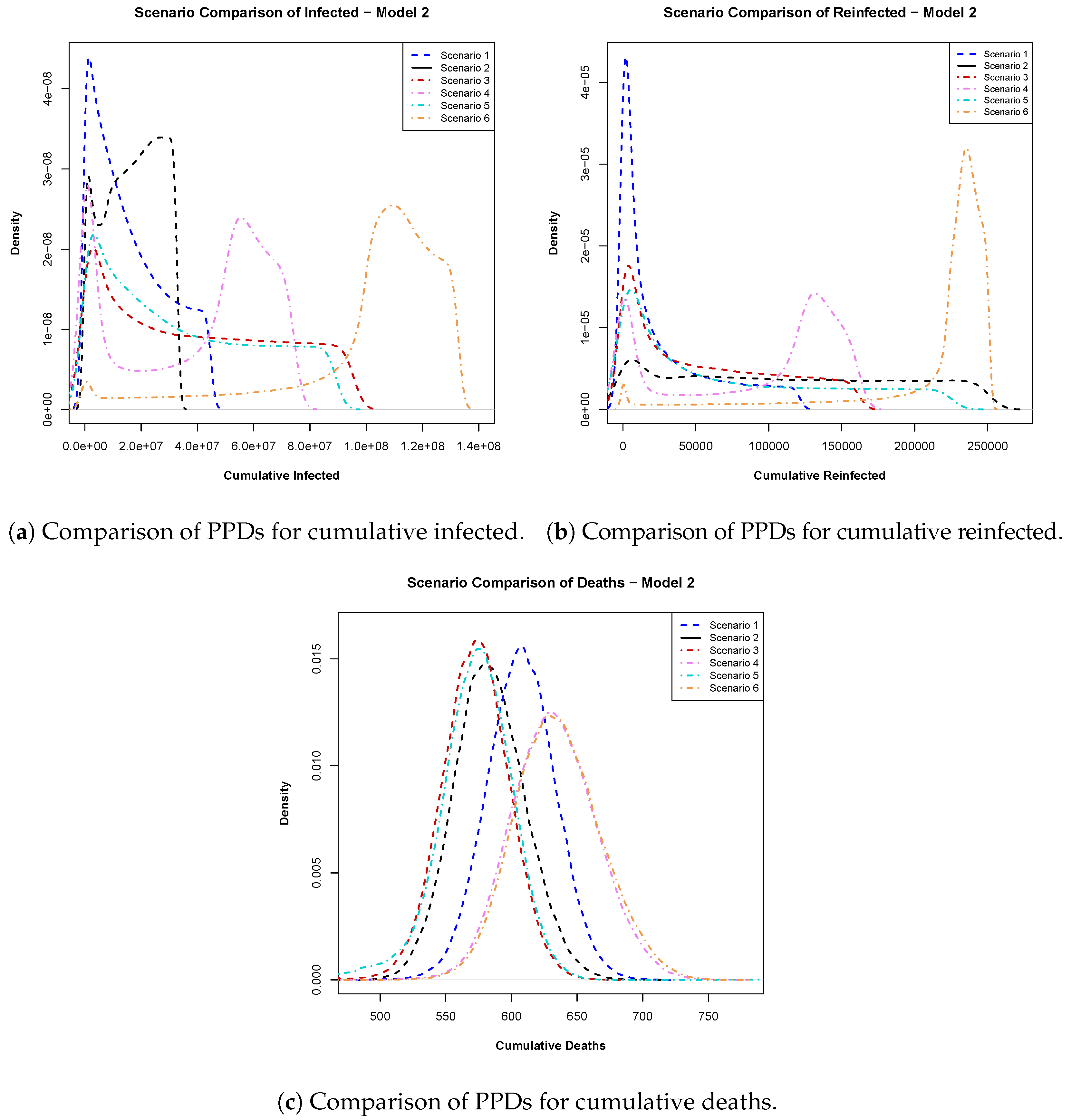
- Model 2: In Figure 6a, the posterior predictive distributions for cumulative infections emphasize the importance of vaccine efficacy, favoring a 100% efficacious vaccine over a 94% efficacious vaccine, regardless of rollout timing. Figure 6b suggests that early vaccination remained preferable due to lower probabilities of excessively high reinfections. Finally, the cumulative PPDs for deaths in Figure 6c advocate for early vaccination with higher-efficacy vaccines, which was shown to result in fewer cumulative deaths.
4.3. Model Comparison Using Bayes Factor
5. Discussion
Author Contributions
Funding
Institutional Review Board Statement
Informed Consent Statement
Data Availability Statement
Acknowledgments
Conflicts of Interest
Appendix A. Details on Hellinger Distance Analysis
References
- Willyard, C. Are repeat COVID infections dangerous? What the science says. Nature 2023, 616, 650–652. [Google Scholar] [CrossRef] [PubMed]
- CDC. About Reinfection. 2024. Available online: https://www.cdc.gov/covid/about/reinfection.html (accessed on 27 April 2025).
- Abu-Raddad, L.J.; Chemaitelly, H.; Bertollini, R. Severity of SARS-CoV-2 reinfections as compared with primary infections. N. Engl. J. Med. 2021, 385, 2487–2489. [Google Scholar] [CrossRef] [PubMed]
- Chemaitelly, H.; Tang, P.; Hasan, M.R.; AlMukdad, S.; Yassine, H.M.; Benslimane, F.M.; Al Khatib, H.A.; Coyle, P.; Ayoub, H.H.; Al Kanaani, Z.; et al. Waning of BNT162b2 vaccine protection against SARS-CoV-2 infection in Qatar. N. Engl. J. Med. 2021, 385, e83. [Google Scholar] [CrossRef] [PubMed]
- Amona, E.B.; Ghanam, R.A.; Boone, E.L.; Sahoo, I.; Abu-Raddad, L.J. Incorporating Interventions to an Extended SEIRD Model with Vaccination: Application to COVID-19 in Qatar. J. Data Sci. 2024, 22, 97–115. [Google Scholar] [CrossRef]
- Ghosh, S.K.; Ghosh, S. A mathematical model for COVID-19 considering waning immunity, vaccination and control measures. Sci. Rep. 2023, 13, 3610. [Google Scholar] [CrossRef]
- Andrews, N.; Stowe, J.; Kirsebom, F.; Toffa, S.; Rickeard, T.; Gallagher, E.; Gower, C.; Kall, M.; Groves, N.; O’Connell, A.M.; et al. COVID-19 vaccine effectiveness against the Omicron (B. 1.1. 529) variant. N. Engl. J. Med. 2022, 386, 1532–1546. [Google Scholar] [CrossRef]
- Hammerman, A.; Sergienko, R.; Friger, M.; Beckenstein, T.; Peretz, A.; Netzer, D.; Yaron, S.; Arbel, R. Effectiveness of the BNT162b2 vaccine after recovery from Covid-19. N. Engl. J. Med. 2022, 386, 1221–1229. [Google Scholar] [CrossRef]
- Hiam, C.; Abu-Raddad, L.J. Waning effectiveness of COVID-19 vaccines. Lancet Infect. Dis. 2022, 22, 1352–1362. [Google Scholar] [CrossRef]
- Lewis, N.; Chambers, L.C.; Chu, H.T.; Fortnam, T.; De Vito, R.; Gargano, L.M.; Chan, P.A.; McDonald, J.; Hogan, J.W. Effectiveness associated with vaccination after COVID-19 recovery in preventing reinfection. JAMA Netw. Open 2022, 5, e2223917. [Google Scholar] [CrossRef]
- Hall, V.; Foulkes, S.; Insalata, F.; Kirwan, P.; Saei, A.; Atti, A.; Wellington, E.; Khawam, J.; Munro, K.; Cole, M.; et al. Protection against SARS-CoV-2 after Covid-19 vaccination and previous infection. N. Engl. J. Med. 2022, 386, 1207–1220. [Google Scholar] [CrossRef]
- Sheehan, M.M.; Reddy, A.J.; Rothberg, M.B. Reinfection rates among patients who previously tested positive for coronavirus disease 2019: A retrospective cohort study. Clin. Infect. Dis. 2021, 73, 1882–1886. [Google Scholar] [CrossRef] [PubMed]
- Rahman, S.; Rahman, M.M.; Miah, M.; Begum, M.N.; Sarmin, M.; Mahfuz, M.; Hossain, M.E.; Rahman, M.Z.; Chisti, M.J.; Ahmed, T.; et al. COVID-19 reinfections among naturally infected and vaccinated individuals. Sci. Rep. 2022, 12, 1438. [Google Scholar] [CrossRef]
- Feikin, D.R.; Higdon, M.M.; Abu-Raddad, L.J.; Andrews, N.; Araos, R.; Goldberg, Y.; Groome, M.J.; Huppert, A.; O’Brien, K.L.; Smith, P.G.; et al. Duration of effectiveness of vaccines against SARS-CoV-2 infection and COVID-19 disease: Results of a systematic review and meta-regression. Lancet 2022, 399, 924–944. [Google Scholar] [CrossRef]
- Mukandavire, Z.; Nyabadza, F.; Malunguza, N.J.; Cuadros, D.F.; Shiri, T.; Musuka, G. Quantifying early COVID-19 outbreak transmission in South Africa and exploring vaccine efficacy scenarios. PLoS ONE 2020, 15, e0236003. [Google Scholar] [CrossRef]
- Chemaitelly, H.; Ayoub, H.H.; Coyle, P.; Tang, P.; Hasan, M.R.; Yassine, H.M.; Al Thani, A.A.; Al-Kanaani, Z.; Al-Kuwari, E.; Jeremijenko, A.; et al. Differential protection against SARS-CoV-2 reinfection pre-and post-Omicron. Nature 2025, 639, 1024–1031. [Google Scholar] [CrossRef]
- Naffeti, B.; Ounissi, Z.; Srivastav, A.K.; Stollenwerk, N.; Van-Dierdonck, J.B.; Aguiar, M. Modeling COVID-19 dynamics in the Basque Country: Characterizing population immunity profile from 2020 to 2022. BMC Infect. Dis. 2025, 25, 9. [Google Scholar] [CrossRef]
- Romero-Ibarguengoitia, M.E.; Rodríguez-Torres, J.F.; Garza-Silva, A.; Rivera-Cavazos, A.; Morales-Rodriguez, D.P.; Hurtado-Cabrera, M.; Kalife-Assad, R.; Villarreal-Parra, D.; Loose-Esparza, A.; Gutiérrez-Arias, J.J.; et al. Association of vaccine status, reinfections, and risk factors with Long COVID syndrome. Sci. Rep. 2024, 14, 2817. [Google Scholar] [CrossRef]
- Xu, Z.; Song, J.; Zhang, H.; Wei, Z.; Wei, D.; Yang, G.; Demongeot, J.; Zeng, Q. A mathematical model simulating the adaptive immune response in various vaccines and vaccination strategies. Sci. Rep. 2024, 14, 23995. [Google Scholar] [CrossRef]
- Wangari, I.M.; Sewe, S.; Kimathi, G.; Wainaina, M.; Kitetu, V.; Kaluki, W. Mathematical modelling of COVID-19 transmission in Kenya: A model with reinfection transmission mechanism. Comput. Math. Methods Med. 2021, 2021, 5384481. [Google Scholar] [CrossRef]
- Tamilalagan, P.; Krithika, B.; Manivannan, P.; Karthiga, S. Is reinfection negligible effect in COVID-19? A mathematical study on the effects of reinfection in COVID-19. Math. Methods Appl. Sci. 2023, 46, 19115–19134. [Google Scholar] [CrossRef]
- Atifa, A.; Khan, M.A.; Iskakova, K.; Al-Duais, F.S.; Ahmad, I. Mathematical modeling and analysis of the SARS-Cov-2 disease with reinfection. Comput. Biol. Chem. 2022, 98, 107678. [Google Scholar] [CrossRef] [PubMed]
- Gelman, A.; Carlin, J.B.; Stern, H.S.; Rubin, D.B. Bayesian Data Analysis; Chapman and Hall/CRC: Boca Raton, FL, USA, 1995. [Google Scholar]
- Gilks, W.R.; Richardson, S.; Spiegelhalter, D. Markov Chain Monte Carlo in Practice; CRC Press: Boca Raton, FL, USA, 1995. [Google Scholar]
- Albert, J. An Introduction to R. In Bayesian Computation with R; Springer: Berlin/Heidelberg, Germany, 2009; pp. 1–17. [Google Scholar]
- Wackerly, D.; Mendenhall, W.; Scheaffer, R.L. Mathematical Statistics with Applications; Cengage Learning: Boston, MA, USA, 2014. [Google Scholar]
- Casella, G.; Berger, R.L. Statistical Inference; Cengage Learning: Boston, MA, USA, 2021. [Google Scholar]
- Berger, J.O. Prior information and subjective probability. In Statistical Decision Theory and Bayesian Analysis; Springer: Berlin/Heidelberg, Germany, 1985; pp. 74–117. [Google Scholar]
- Jeffreys, H. The Theory of Probability; OuP: Oxford, UK, 1998. [Google Scholar]
- Lesaffre, E.; Lawson, A.B. Bayesian Biostatistics; John Wiley & Sons: Hoboken, NJ, USA, 2012. [Google Scholar]
- Kass, R.E.; Raftery, A.E. Bayes factors. J. Am. Stat. Assoc. 1995, 90, 773–795. [Google Scholar] [CrossRef]
- Goutis, C.; Robert, C.P. Model choice in generalised linear models: A Bayesian approach via Kullback-Leibler projections. Biometrika 1998, 85, 29–37. [Google Scholar] [CrossRef]
- Goldenberg, I.; Webb, G.I. Survey of distance measures for quantifying concept drift and shift in numeric data. Knowl. Inf. Syst. 2019, 60, 591–615. [Google Scholar] [CrossRef]
- Birgé, L. On estimating a density using Hellinger distance and some other strange facts. Probab. Theory Relat. Fields 1986, 71, 271–291. [Google Scholar] [CrossRef]
- Boone, E.L.; Merrick, J.R.; Krachey, M.J. A Hellinger distance approach to MCMC diagnostics. J. Stat. Comput. Simul. 2014, 84, 833–849. [Google Scholar] [CrossRef]
- Scott, D.W. Multivariate Density Estimation: Theory, Practice, and Visualization; John Wiley & Sons: Hoboken, NJ, USA, 2015. [Google Scholar]
- Abu-Raddad, L.J.; Chemaitelly, H.; Butt, A.A. Effectiveness of the BNT162b2 Covid-19 Vaccine against the B. 1.1. 7 and B. 1.351 Variants. N. Engl. J. Med. 2021, 385, 187–189. [Google Scholar] [CrossRef]
- LaJoie, Z.; Usherwood, T.; Sampath, S.; Srivastava, V. A COVID-19 model incorporating variants, vaccination, waning immunity, and population behavior. Sci. Rep. 2022, 12, 20377. [Google Scholar] [CrossRef]
- Burch, E.; Khan, S.A.; Stone, J.; Asgharzadeh, A.; Dawe, J.; Ward, Z.; Brooks-Pollock, E.; Christensen, H. Mathematical models of COVID-19 vaccination in high-income countries: A systematic review. medRxiv 2024. [Google Scholar] [CrossRef]
- Wang, X.; Du, Z.; Johnson, K.E.; Pasco, R.F.; Fox, S.J.; Lachmann, M.; McLellan, J.S.; Meyers, L.A. Effects of COVID-19 vaccination timing and risk prioritization on mortality rates, United States. Emerg. Infect. Dis. 2021, 27, 1976. [Google Scholar] [CrossRef]

| Compartment | Initial Conditions | Source |
|---|---|---|
| 2,695,122 | Population of Qatar as of 30 December 2022 | |
| 2,695,122/6 | Assumed | |
| 0 | From the data | |
| 5 | From [5] | |
| 1 | From the data | |
| 0 | From the data | |
| 0 | From the data | |
| 0 | From the data | |
| 0 | From the data |
| Model | Parameter | Description | Est. Mean | Psuedo- | |
|---|---|---|---|---|---|
| Model 1 | Transmission rate before intervention | () | |||
| Transmission rate after the first intervention | () | ||||
| Transmission rate after the second intervention | () | ||||
| Transmission rate after the third intervention | () | ||||
| Transmission rate after the fourth intervention | () | ||||
| Transmission rate after the fifth intervention | () | ||||
| Transmission rate after the sixth intervention | () | ||||
| Transmission rate after the seventh intervention | () | ||||
| Transmission rate after the eighth intervention | () | ||||
| Transmission rate after the ninth intervention | () | ||||
| Rate at which the exposed become infectious | () | ||||
| Recovery rate from infections influenced by intervention | () | ||||
| Recovery rate from infections influenced by intervention | () | ||||
| Recovery rate from infections influenced by intervention | () | ||||
| Recovery rate from infections influenced by intervention | () | ||||
| Reinfection rate influenced by intervention | () | ||||
| Reinfection rate influenced by intervention | () | ||||
| Reinfection rate influenced by intervention | () | ||||
| Reinfection rate influenced by intervention | () | ||||
| Recovery rate from reinfections | () | ||||
| Vaccination rate | () | ||||
| Vaccine efficacy | () | ||||
| Death rate | () | ||||
| Waning rate of natural immunity | () | ||||
| Waning rate of immunity due to vaccination | () | ||||
| Transmission rate before intervention | () | ||||
| Transmission rate after the first intervention | () | ||||
| Transmission rate after the second intervention | () | ||||
| Transmission rate after the third intervention | () | ||||
| Transmission rate after the fourth intervention | () | ||||
| Transmission rate after the fifth intervention | () | ||||
| Transmission rate after the sixth intervention | () | ||||
| Transmission rate after the seventh intervention | () | ||||
| Transmission rate after the eighth intervention | 00114 | () | |||
| Transmission rate after the ninth intervention | () | ||||
| Infectious rate | () | ||||
| Recovery rate from infections influenced by intervention | () | ||||
| Model 2 | Recovery rate from infections influenced by intervention | () | |||
| Recovery rate from infections influenced by intervention | () | ||||
| Recovery rate from infections influenced by intervention | () | ||||
| Reinfection rate influenced by intervention | () | ||||
| Reinfection rate influenced by intervention | () | ||||
| Reinfection rate influenced by intervention | () | ||||
| Reinfection rate influenced by intervention | () | ||||
| Recovery rate from reinfections | () | ||||
| Vaccination rate | () | ||||
| Vaccine efficacy | () | ||||
| Death rate | () | ||||
| Waning rate of natural immunity | () | ||||
| Waning rate of immunity due to vaccination | () |
Disclaimer/Publisher’s Note: The statements, opinions and data contained in all publications are solely those of the individual author(s) and contributor(s) and not of MDPI and/or the editor(s). MDPI and/or the editor(s) disclaim responsibility for any injury to people or property resulting from any ideas, methods, instructions or products referred to in the content. |
© 2025 by the authors. Licensee MDPI, Basel, Switzerland. This article is an open access article distributed under the terms and conditions of the Creative Commons Attribution (CC BY) license (https://creativecommons.org/licenses/by/4.0/).
Share and Cite
Amona, E.B.; Sahoo, I.; Boone, E.L.; Ghanam, R. Studying Disease Reinfection Rates, Vaccine Efficacy, and the Timing of Vaccine Rollout in the Context of Infectious Diseases: A COVID-19 Case Study. Int. J. Environ. Res. Public Health 2025, 22, 731. https://doi.org/10.3390/ijerph22050731
Amona EB, Sahoo I, Boone EL, Ghanam R. Studying Disease Reinfection Rates, Vaccine Efficacy, and the Timing of Vaccine Rollout in the Context of Infectious Diseases: A COVID-19 Case Study. International Journal of Environmental Research and Public Health. 2025; 22(5):731. https://doi.org/10.3390/ijerph22050731
Chicago/Turabian StyleAmona, Elizabeth B., Indranil Sahoo, Edward L. Boone, and Ryad Ghanam. 2025. "Studying Disease Reinfection Rates, Vaccine Efficacy, and the Timing of Vaccine Rollout in the Context of Infectious Diseases: A COVID-19 Case Study" International Journal of Environmental Research and Public Health 22, no. 5: 731. https://doi.org/10.3390/ijerph22050731
APA StyleAmona, E. B., Sahoo, I., Boone, E. L., & Ghanam, R. (2025). Studying Disease Reinfection Rates, Vaccine Efficacy, and the Timing of Vaccine Rollout in the Context of Infectious Diseases: A COVID-19 Case Study. International Journal of Environmental Research and Public Health, 22(5), 731. https://doi.org/10.3390/ijerph22050731