Article

First Steps towards a near Real-Time Modelling System of Vibrio vulnificus in the Baltic Sea

by
Eike M. Schütt
1,*,
Marie A. J. Hundsdörfer
1,
Avril J. E. von Hoyningen-Huene
2,
Xaver Lange
3,
Agnes Koschmider
4 and
Natascha Oppelt
1
1
Earth Observation and Modelling, Department of Geography, Kiel University, 24118 Kiel, Germany
2
Molecular Microbiology, Institute for General Microbiology, Kiel University, 24118 Kiel, Germany
3
Leibniz Institute for Baltic Sea Research Warnemünde, 18119 Rostock, Germany
4
Business Informatics and Process Analytics, University of Bayreuth, 95447 Bayreuth, Germany
*
Author to whom correspondence should be addressed.
Int. J. Environ. Res. Public Health 2023, 20(8), 5543; https://doi.org/10.3390/ijerph20085543
Submission received: 28 February 2023 / Revised: 24 March 2023 / Accepted: 10 April 2023 / Published: 17 April 2023
(This article belongs to the Special Issue Marine Ecology and Health)

Abstract

:
Over the last two decades, Vibrio vulnificus infections have emerged as an increasingly serious public health threat along the German Baltic coast. To manage related risks, near real-time (NRT) modelling of V. vulnificus quantities has often been proposed. Such models require spatially explicit input data, for example, from remote sensing or numerical model products. We tested if data from a hydrodynamic, a meteorological, and a biogeochemical model are suitable as input for an NRT model system by coupling it with field samples and assessing the models’ ability to capture known ecological parameters of V. vulnificus. We also identify the most important predictors for V. vulnificus in the Baltic Sea by leveraging the St. Nicolas House Analysis. Using a 27-year time series of sea surface temperature, we have investigated trends of V. vulnificus season length, which pinpoint hotspots mainly in the east of our study region. Our results underline the importance of water temperature and salinity on V. vulnificus abundance but also highlight the potential of air temperature, oxygen, and precipitation to serve as predictors in a statistical model, albeit their relationship with V. vulnificus may not be causal. The evaluated models cannot be used in an NRT model system due to data availability constraints, but promising alternatives are presented. The results provide a valuable basis for a future NRT model for V. vulnificus in the Baltic Sea.

1. Introduction

Vibrio spp. are ubiquitous members of the ocean and freshwater microbial communities. More than 100 different Vibrio species have been identified [1]. They occur free-living in the water column or are attached to biotic or abiotic surfaces [2,3]. Vibrio spp. play an important role in marine nutrient cycles [4,5], and some species are known to form symbiotic relationships with marine animals (e.g., Aliivibrio fischeri and squids) [6]. About a dozen Vibrio spp. are human pathogens [1,7,8]. For example, two serogroups of Vibrio cholerae (O1 and O139) are the causative agents of the intestinal disease cholera [1]. Non-O1, non-O139 V. cholera strains and other Vibrio spp. cause vibriosis, with symptoms ranging from gastroenteritis to skin and soft tissue infections with necrotizing fasciitis, septicaemia, or even fatal septic multi-organ failure [7,9]. Infection pathways include handling and consumption of contaminated raw seafood as well as direct exposure to seawater [1,10].
Vibriosis outbreaks in Northern Europe are often attributed to V. alginolyticus, V. cholerae (non-O1/non-O139), V. parahaemolyticus, and V. vulnificus [11,12,13]. The number of incidents is generally low. However, infections with the species V. vulnificus are often severe (>90% of all cases) and have high mortality rates [9,12,13]. Therefore, vibriosis, particularly vibriosis linked to V. vulnificus, is a public health concern [13]. Empirical evidence of increased infection rates in warmer summers indicates that this problem will gain traction in the coming decades [11,12,13,14,15,16].
Understanding the ecology of Vibrio, which causes vibriosis, particularly of V. vulnificus, and predicting their abundance is an important component for the effective management of Vibrio-related public health risks [17]. With growth rates of up to several generations per hour, Vibrio vulnificus is known to form short but intense blooms under favorable conditions [18,19]. It has commonly been observed that favourable conditions consist of water temperatures above approximately 20 °C and salinity ranging from 5–25 practical salinity units (PSU) [19,20,21,22,23]. The predictive power of other variables, such as turbidity, chlorophyll a (Chl), dissolved organic carbon (DOC), or concentrations of nutrients, varies between study regions, indicating that limiting factors differ between habitats [2].
The Baltic Sea has low salinity and one of the highest warming rates in marine ecosystems worldwide [24]; thus, it is considered a high-risk environment for vibriosis infections [13,14]. In recent years, infection numbers have increased significantly along the German Baltic coast, particularly during heatwaves [12,15]. Infection risk management along the German Baltic Sea includes regular V. vulnificus quantification from water samples at seven beaches in the federal state of Mecklenburg–Western Pomerania (MV) during the summer months, and awareness campaigns for visitors [25]. In the federal state of Schleswig-Holstein (SH), samples have only been collected following reported cases of vibriosis and during irregular scientific projects [26].
Advances in remote sensing and model products provide opportunities for modelling of Vibrio abundances and infection risks in near real-time (NRT) [27]. One example is the Vibrio Map Viewer provided by the European Centre for Disease Prevention and Control (https://geoportal.ecdc.europa.eu/vibriomapviewer/, accessed on: 18 January 2023). It provides a species-independent relative Vibrio infection risk index. The index is calculated based on sea surface temperature (SST) and sea surface salinity (SSS) from remote sensing products, as well as ocean reanalysis and forecast products [16]. However, this species-independent approach may be inaccurate as individual Vibrio spp. show different responses to the same environmental conditions [17,21,28,29]. Moreover, as vibriosis infections are likely to be under-reported and infection risks have sociological, demographic, and behavioural components [12,13,17,30], modelling Vibrio occurrence probabilities or quantities of a certain species may provide more robust results for NRT modelling.
Despite suggestions that creating an operational NRT modelling system for V. vulnificus quantities in the Baltic Sea would be a step towards better management of the increasing risks of Vibrio-related public health issues in the future [12,13,15,17,22,27], no such attempts have been made. This study aims to pave the way towards a spatially resolved monitoring system. Such a monitoring system has to rely on observations from satellites or on model outputs. In this study, we test whether we can use a hydrodynamic model, a biogeochemical model, and a meteorological reanalysis to identify known ecological characteristics of V. vulnificus by coupling the model data with more than 600 samples of V. vulnificus. Moreover, we identify parameters particularly suited for predicting V. vulnificus abundances in the western Baltic Sea by applying a novel network detection method, the St. Nicolas House Analysis [31]. We discuss the suitability of the applied model data for an NRT modelling system for V. vulnificus and offer suggestions for improvements. Moreover, using a time series of 27 years of modelled daily SST, based on validated hindcast simulations, we attempt to detect the footprint of climate change on V. vulnificus season length and detect hotspots of frequent V. vulnificus occurrence along the German Baltic coast.

2. Materials and Methods
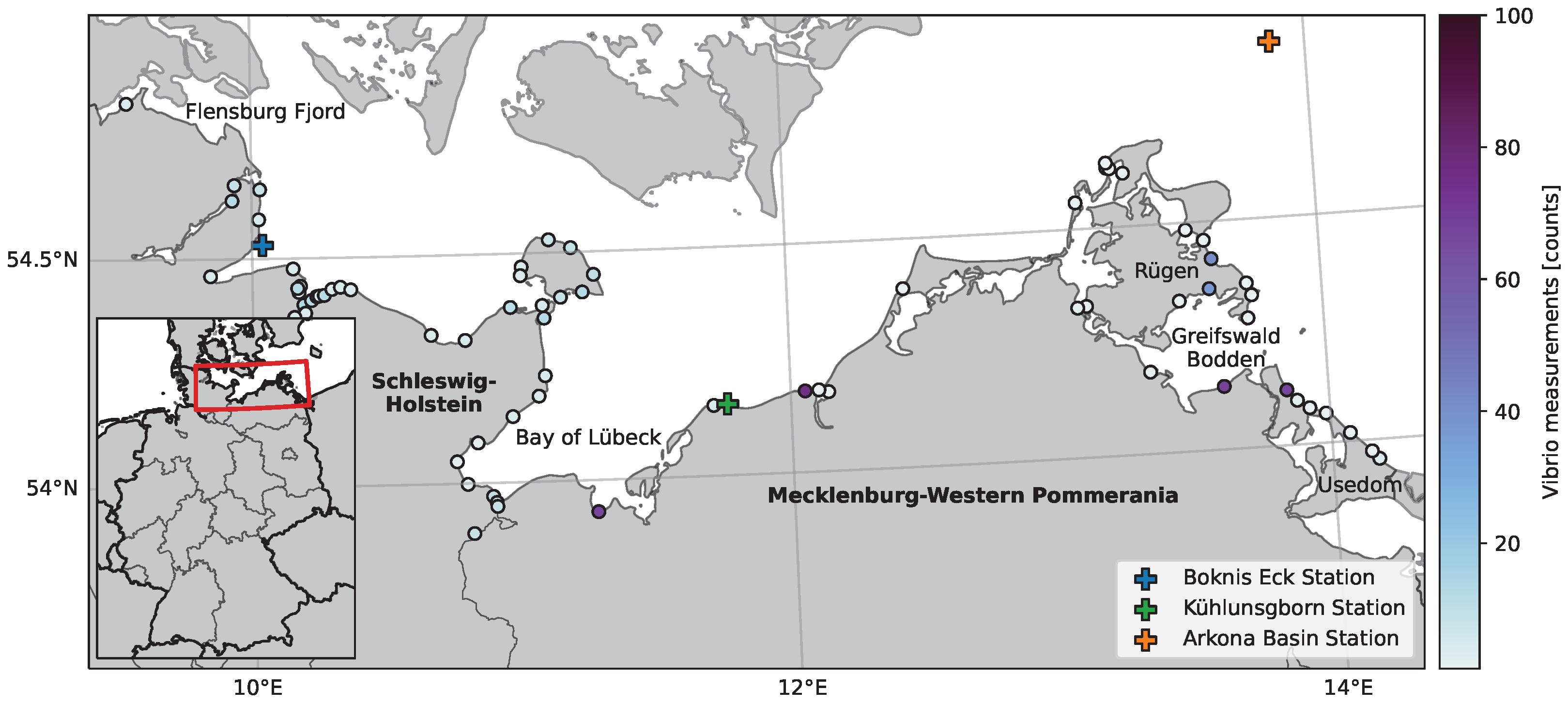
The following section outlines the study area, materials, and methodology used to identify the environmental drivers of V. vulnificus in the south-western Baltic Sea. A list of abbreviations and acronyms is provided at the end of the article.

2.1. Study Area

The German coast of the Baltic Sea is characterised by large bights, the “Schlei” (a narrow inlet in the north-west of the study region of ∼30 km length), fjords, and the shallow “Bodden” in the east (Figure 1). The latter are briny, lagoon-like water bodies with complex morphologies, which naturally experience limited mixing between the sea and river estuaries. The Baltic Sea’s salinity relies solely on inflow events from North Sea water through the Kattegat. Hence, a strong salinity gradient from west to east is present in our study area. In the northwest of the study area, the average SSS is around 16–19 PSU; however, it can vary significantly due to wind-driven currents [32,33]. Towards the east of the study area, the mean SSS decreases along with its variability to values as low as 7 PSU in the open Baltic Sea. In the inlets, estuaries, and Bodden, the influx of riverine freshwater reduces the salinity even further [34].
SST shows strong seasonal dynamics. During the summer months, SST reaches averages of 17 °C in the open sea and up to 20 °C in sheltered and shallow areas. Heatwaves may cause positive SST anomalies of up to 5 °C, as observed in 2018 [12,22]. The combination of SST during the summer months and moderate salinity provides ideal conditions for V. vulnificus [14,20]. Moreover, large parts of the Baltic Sea are affected by eutrophication, indicating high nutrient availability [35].

2.2. V. vulnificus Quantification

The Vibrio datasets used in this study were provided by the Ministry of Social Affairs, Youth, Family, Senior Citizens, Integration and Equality Schleswig-Holstein (SoZMI), and the State Agency for Health and Social Affairs Mecklenburg–Western Pomerania (LAGuS). The former dataset consists of samples taken along the Baltic coast of the German state of Schleswig-Holstein (SH) between 2014 and 2021. The latter provides measurements from Mecklenburg–Western Pomerania (MV) between 2008 and 2021. Samples were taken during several independent monitoring projects of the federal states, which used different sampling periods and cultivation-based identification and quantification of Vibrio spp., as described in the following. The SH dataset contains samples from a campaign in 2014 and incident-based samples from 2015 to 2021. Incident-based samples were taken after reported cases of Vibrio infections. For Vibrio quantification and species identification, 250 mL of water was sampled from bathing areas at 30 cm below the surface according to SH bathing water directive BadGewQualV SH [36]. Moreover, 1–2 mL of the sample were filtered through membrane filters with a pore size of 0.45 µM (Millipore, Burlington, MA, USA). Filters and 200 µL of an undiluted sample were plated onto CHROMagarTM Vibrio (CHROMagar, Paris, France) and incubated for 24 h at 36 °C and 5% CO 2 . Colourimetrically positive colonies were subcultured onto Marineagar (DifcoTM Marine Broth with 1.5% Agar–Agar, both BD Diagnostics, Franklin Lakes, NJ, USA) for a further 24 h. The colonies of Vibrio species (V. parahaemolyticus, V. vulnificus, and V. cholerae) were counted, and colony-forming units (CFUs) extrapolated for 1 ml seawater (CFU/mL). Vibrio identity was verified using individual colonies and a MALDI-TOF analysis (see [37] for further information on sampling, cultivation, and identification of Vibrio). In MV, water samples were taken every 2 weeks at 7 stations starting in 2008. Sampling began each summer after a threshold water temperature of 17–18 °C was reached [25]. Vibrio identification and quantification in water samples was done using a cultivation-based approach, similar to the SH dataset. For a description of the cultivation, refer to [38]. While the CFU/mL was calculated in the SH dataset, the MV dataset estimated V. vulnificus abundance in powers of 10 (the most probable number technique). This entailed screening Vibrio growth along a dilution series and recording the highest dilution with visible colonies. The experiments were conducted in triplicate. To make the SH and MV datasets comparable, the SH records were converted into corresponding powers of ten.
Quantitative measurements were mostly only available for V. vulnificus, which is also the dominant potentially human-pathogenic Vibrio spp. in the south-western Baltic Sea [22]. Other Vibrio spp. were only recorded as present/absent in a sample. Thus, we focused on working with samples of V. vulnificus only.

2.3. Environmental Data

To explore the relationship between environmental factors and V. vulnificus response, data for 11 parameters were extracted from models and reanalysis, including freely available biogeochemical and meteorological reanalysis products (Table 1). Special emphasis was put on SST and SSS, which have been identified as the most important parameters driving V. vulnificus abundance in several studies (e.g., reference [2] and references therein). To reflect this, a high-resolution hydrodynamic model was used to resolve coastal areas and narrow inlets. The following sections will briefly present the different model systems.

2.3.1. High-Resolution Hydrodynamic Model

The General Estuarine Transport Model (GETM) [41,42] was used to simulate SST and SSS in the western Baltic Sea from 1995 to 2021. The 3D simulations used a horizontal resolution of 200 m on a spherical grid with 35 depth layers, which were adapted to vertical density gradients [42,43]. Turbulence closure (second-order, k- ε ) was implemented by using the General Ocean Turbulence Model [44,45]. Boundary conditions at the open boundaries were taken from a larger-scale model of the Baltic Sea (see [32] for details).
Model results were validated with in situ data from three in situ sampling stations (Figure 1). At Boknis Eck, the modelled data were compared to monthly measurements of temperature and salinity at 1 m depth (https://www.bokniseck.de/, accessed on: 27 November 2022) [46]. The Leibniz Institute for Baltic Sea Research Rostock, Germany, provided daily mean water temperatures for the Kühlungsborn station measured at a 1 m depth. At the Arkona Basin station, part of the Marine Environmental Monitoring Network [47], daily averages of the shallowest available measurement depths of water temperature and salinity (0.5 m and 2 m, respectively) were used in the validation exercise. To asses the model accuracy, we calculated the Pearson correlation coefficient (r), mean absolute error (MAE), and bias between modelled and observed data.

2.3.2. Biogeochemical Data

Data on nutrients, dissolved oxygen (O 2 ), and Chl (a proxy for phytoplankton biomass [48]) were taken from a biogeochemical reanalysis product for the Baltic Sea produced by the Copernicus Marine Environment Monitoring Service CMEMS [39]. The reanalysis product is based on the Nucleus for European Modelling of the Ocean (NEMO) circulation model in the NEMO-Nordic configuration [49,50], coupled with the Swedish Coastal and Ocean Biogeochemical model [51,52]. The model is forced with meteorological data and observations, including SST charts and in situ measurements of temperatures and several chemical parameters [53]. The model domain covers the entire Baltic Sea and its transition to the North Sea. It resolves up to 56 depth layers and has provided daily averages of NO 3 , PO 4 , NH 4 , O 2 , and Chl since 1993 at a spatial resolution of approximately 4 × 4 km.
We accessed the dataset through CMEMS OPeNDAP Python API and downloaded all daily averages of the surface layer in our study region since the beginning of the V. vulnificus sampling program in 2008.

2.3.3. Meteorological Data

The COSMO-REA6 dataset is a reanalysis product from the German Weather Service DWD [40]. It is based on the COSMO (Consortium for Small-scale Modelling) numerical weather prediction model and a data assimilation scheme that incorporates observations from various sources, such as weather stations, ships, and aircraft. The model domain covers Europe and northern Africa with a spatial resolution of 6 × 6 km. Hourly data are available for the period between 1995 and August 2019.
We downloaded daily averages of surface air temperature (SAT), total precipitation, solar irradiation, and wind speed (calculated from u and v components) for the study period (2008–2019) from the open data server of the DWD (https://opendata.dwd.de/climate_environment/REA/, accessed on: 6 December 2022).

2.3.4. Aggregation of Environmental Data and Identification of Lead Time

Several studies indicate a lead time between some environmental parameters (e.g., air temperature) and V. vulnificus abundance [21,38,54]. For this reason, time series of all environmental parameters from the 30 days before a V. vulnificus sampling time were extracted for each sampling to calculate the lead time with the highest predictive power for each parameter. Due to the spatial resolution of the GETM and CMEMS Biogeochemistry Reanalysis products (200 × 200 m and 4 × 4 km, respectively), valid data was not always available directly at the coastal sampling locations. In such situations, all data within a predefined radius around the sampling location were averaged. The search distance was increased iteratively until valid predictions were found or a maximum radius of 1.5 × the grid cell resolution was reached.
The 30-day time series were analysed using a moving window of flexible size (Figure 2). For each window, the average (for precipitation, the sum) was calculated, correlated with V. vulnificus quantities, and plotted in correlation matrices. Spearman’s rank correlation was used to account for potential non-linearity of underlying processes. The window with the highest correlation coefficient was generally used as the time lag in further analysis.
It has already been observed that V. vulnificus quantities not only depend on absolute values of a parameter, but also on the duration of an event [19,55]. Therefore, we chose to not only consider absolute values of environmental parameters but also their trends by estimating the slope of a linear least squares fit. The trend was calculated for each moving window of flexible size, and we identified the window with the highest correlation coefficient using Spearman’s rank correlation.
Previous studies in temperate regions have shown that V. vulnificus enters a viable but non-culturable state (VBNC), which is a survival strategy altering their metabolism if water temperatures drop below ∼13–15 °C [56]. For resuscitation, the cells require considerably higher temperatures (∼17–20 °C). To capture this seasonal dynamic, an additional parameter containing the maximum SST of the past weeks and months was added. The best window was determined with the same workflow as described above, but on a time series covering the period of 30 to 300 days before sampling.
In the following, lag windows of variables will be denoted as, for instance, SSTmean12–15. This stands for the average SST between 12 and 15 days before Vibrio sampling.

2.4. Statistical Analysis

Initially, we tested the ability of our models to reproduce known ecological characteristics of V. vulnificus by calculating Spearman’s rank correlation coefficient ( r s ) between all parameters and plotting V. vulnificus quantities over SST and SSS in a bubble plot. Ecological preferences and distribution boundaries were then compared with literature studies from temperate regions. We then identified parameters associated with V. vulnificus quantities using the Saint Nicolas House Analysis (SNHA). SNHA provides an approach for initial data analysis by visualizing associations between variables in non-linear multivariate data [31]. It ranks absolute bivariate correlation coefficients in descending order according to the magnitude and creates hierarchical association chains. These association chains must also be reversible, i.e., the same order must be derived if the end node (i.e., an environmental parameter in our study) of a chain becomes the start node. Superimposing all detected chains creates a network graph, which can be used to characterize and visualize dependencies between interacting variables, as described by Hermanussen et al. [57]. In contrast to similar approaches, SNHA is non-parametric, robust to outliers, and relatively robust against spurious significance [31,57].
Recently, Hake et al. [58] proposed an improvement for the detection of branched association chains in densely interconnected networks using a bootstrapping routine. Bootstrapping involves randomly selecting samples with replacements from the original dataset. In each re-sampling, SNHA is applied, and the detected edges (i.e., connections between nodes) are counted across all re-samplings. An edge becomes significant if it is detected more than λ times. λ is estimated using a binomial test and depends mainly on the number of bootstrap iterations and the probability of success (i.e., the probability an edge is falsely detected).
SNHA was applied to the complete dataset of V. vulnificus samples and environmental parameters to unveil a network between the different parameters. We used the Python implementation SNHA4py (https://github.com/thake93/snha4py, accessed on: 3 January 2023, v20230103) [58] and the bootstrapping routine with 100 iterations. The binomial test with a probability of success of 0.035 (derived empirically by Hake et al. [58]) suggested that edge predictions made in more than 8% of all iterations are statistically significant ( p < 0.05 ).
Preliminary results identified SST as the most important parameter determining V. vulnificus quantity. Our high-resolution SST product provides the unprecedented opportunity to identify hotspots with frequently favourable SST and regions with high warming rates since 1995. To identify these regions, we first calculated the V. vulnificus occurrence probability with logistic regression on our V. vulnificus samples and corresponding modelled SST values from our GETM realisation. Next, we counted the days in each year where SST exceeded the temperature of the 33% probability of V. vulnificus occurrence (from hereon referred to as season length; the selection of the threshold will be discussed later). Trends were estimated with Sen’s slope, and their statistical significance was ensured with the Mann–Kendall test using the pyMannKendall package [59].

3. Results

3.1. Validation of the Hydrodynamic Model

Validation of the high-resolution hydrodynamic model demonstrates the accuracy of both SST and SSS products (Figure 3). Both parameters are strongly correlated with in situ data (r of 0.99 and 0.97 for SST and SSS, respectively). However, the model appears to slightly underestimate SST (bias = −0.1 °C, MAE = 0.66 °C). For SSS, the MAE is approximately 0.4 PSU and the bias is negligible (−0.03 PSU), although SSS at Boknis Eck appears to be moderately overestimated (bias of 1.88 PSU).
Figure 4 shows the average SST during the summer months (June–August) and the average SSS. The SST patterns appear reasonable, with higher temperatures in shallow and sheltered bays and lower temperatures in offshore areas with greater depths. In the northwest of the study area, relatively low SSTs close to the shore can be attributed to frequent local upwelling events during the summer months [60]. The SSS climatology closely depicts the salinity gradient along the German Baltic coast. However, the model results indicate low salinity (nearly 0 PSU) for three narrow inlets (areas marked with hashed lines in Figure 4), which contradicts published salinity measurements from these areas [34]. This discrepancy may be caused by the model’s underestimation of the water exchange between the open Baltic Sea and these bays, as the narrowest inlet of all three areas is smaller than the model’s grid resolution of 200 m. Therefore, these specific bays were excluded from the subsequent analysis.

3.2. Analysis of Lag Windows and SNHA

Data of all environmental parameters were available for a total of 621 V. vulnificus samples (408 in MV and 213 in SH). For each environmental parameter, we created correlation matrices with V. vulnificus quantities. In most cases, the lag window with the highest r s was chosen for further analysis. For the parameters SST t r e n d , PO 4 t r e n d , and Chl m e a n , we selected considerably longer window lengths with slightly lower r s (see Table A1 for details).
With the selected lag windows, we calculated a correlation matrix with V. vulnificus quantities and all environmental parameters (Figure A2). All environmental parameters, except Chlmean6–15 (i.e., mean Chl between 6 and 15 days before Vibrio sampling), correlate significantly with V. vulnificus quantity (p > 0.05), albeit most r s are low. Parameters with the highest absolute r s are SSTmean0–11, SATmean0–16, O2mean0–0 and SSSmean0–6 ( r s of 0.55, 0.49, −0.37, and −0.35, respectively).
Figure 5 shows the abundance of V. vulnificus in relation to both SST and SSS. The probability that V. vulnificus occurs increases with higher SST, starting from ∼17 °C. At 19 °C, V. vulnificus was detected in about 60% of all samples. The lowest temperature at which V. vulnificus could be detected was 14.1 °C. In contrast to temperature, V. vulnificus was observed across almost the entire salinity gradient of the study area (3.7–19.4 PSU).
We applied SNHA to derive a network between all parameters (Figure 6). The mean sea surface temperature (more specifically SSTmean0–11) forms the centre of the network and is connected to 10 other parameters, including biogeochemical, meteorological, and physical parameters, as well as the V. vulnificus quantity. The biogeochemical parameters sharing an edge with SST are mean oxygen (O 2 mean0–0), mean nitrate (NO 3 mean7–25), mean ammonium (NH 4 trend9–10), and the oxygen trend (O 2 trend5–16). The meteorological parameters include mean surface air temperature (SATmean0–16), wind speed (WSmean2–17), and the trend of surface air temperature (SATtrend7–29). The physical parameters connected to the mean sea surface temperature are the sea surface temperature 180 days before sampling (SST 180 ) and the trend of sea surface salinity (SSStrend11–26). With an r s of 0.88, the average sea surface temperature (SSTmean0–11) and surface air temperature (SATmean0–16) are closely related.
Direct edges to V. vulnificus were inferred from seven parameters. Among them are mean sea surface temperature (SSTmean0–11, r s of 0.55), mean surface air temperature (SATmean0–16, r s of 0.49), mean oxygen concentration (O 2 mean0–0, r s of −0.37), mean sea surface salinity (SSSmean0–6, r s of −0.35), surface temperature 180 days before sampling (SST 180 , r s of −0.35), average precipitation (Precmean6–18, r s of −0.21), and the trend of precipitation (Prectrend5–8, r s of −0.16). The correlations of all these edges are significant at the p < 0.001 level. There is no direct edge between V. vulnificus quantity and nutrients or Chl. However, mean ammonium (NH4mean28–28), phosphate (PO4mean22–22), nitrate (NO3mean7–25), and chlorophyll (Chlmean6–15) have a link to mean sea surface salinity (SSSmean0–6), while mean nitrate (NO3mean7–25) and the trend of ammonium (NH4trend9–10) are connected to the average sea surface temperature SSTmean0–11. These nutrients are, thus, indirectly connected to the V. vulnificus quantity.

3.3. Trends of the V. vulnificus Season Length

To describe the length of the V. vulnificus season, we calculated the occurrence probability based on SST with logistic regression. The fit reveals a slow increase of occurrence probability up to ∼17 °C. At 17.6 °C, the probability reaches 33% and increases sharply by about 20% per degree (Figure A1).
Figure 7 displays the V. vulnificus season length (i.e., days with SST > 17.6 °C) for 1995 (a) and 2021 (b). Apart from the trend towards a longer season in 2021, the season length exhibits similar geographic patterns in both years. Longer than average seasons occurred, for example, in the inner Flensburg Fjord in the north-west of the study region, the Bay of Lübeck in the centre, and the easternmost areas of the study region (see labels in Figure 1 for the locations of these regions). Relatively short seasons can be observed in some inlets in the west of the study region, near the Danish islands of Lolland and Falster, and in the north-west of the island Rügen. Figure 7c indicates a trend towards a longer V. vulnificus season in virtually the entire German Baltic Sea, although in most areas, the trends are not significant (Figure 7d). The most distinct area with a significant increase in season length is located in the east of the study area, close to the island of Usedom. Smaller areas with significant increases are located in sheltered and shallow bays with limited water exchange (e.g., Greifswald Bodden or Flensburg Fjord) and in the extension of the estuary of the river Warnow. The fastest season expansion was calculated for the inner Flensburg Fjord, increasing at a rate of up to 1.4 days per year.

4. Discussion

This study represents an initial step towards developing a spatially explicit near real-time (NRT) modelling system for the German Baltic Sea by combining more than 600 V. vulnificus samples from the Baltic coast with modelled data of environmental parameters such as SST, SSS, and nutrient concentrations. On the one hand, this allows evaluating the suitability of the models to resolve key ecological characteristics of V. vulnificus. On the other, it can pinpoint ecological parameters that are best suited for predicting V. vulnificus occurrences in the Baltic Sea using a statistical model.

4.1. Ecological Characteristics of V. vulnificus in the South-Western Baltic Sea

Our results largely confirm the important constraining influence of SST on V. vulnificus abundance in regions with a temperature-driven seasonal cycle, e.g., [20,61,62]. In fact, we identified SST m e a n 0 11 to be the most limiting parameter in our region of study. The probability of V. vulnificus occurrence increased rapidly once SST exceeded ∼17 °C. The highest numbers of V. vulnificus CFUs were observed when SST was above 20 °C. These dynamics agree well with reports from other studies, e.g., [21,22,63].
After proliferating in the summer months, V. vulnificus can persist at lower temperatures before entering the VBNC state. Oliver et al. [56] reported that the transition into the VBNC state occurs at around 15 °C SST. These results have been confirmed by studies in Barnegat Bay, USA (12 °C in [20]) and in the German North Sea (14 °C in [21] and 13 °C in [29]). The 14 °C detection limit determined by the model in this study is thereby confirmed by commonly observed experimental values. To capture the seasonal effect of a larger tolerance of V. vulnificus towards lower water temperatures in autumn before entering the VBNC state, we included SST 180 days before sample acquisition (SST 180 ) as a parameter in the SNHA analysis. Indeed, SNHA inferred an edge between SST 180 and V. vulnificus quantity. This indicates that SST 180 takes into consideration different aspects of the variability in V. vulnificus quantities, such as season, which are not detected by SST with no or minimal lag. It may, therefore, be a valuable additional predictor in a statistical NRT model.
SNHA also detected an edge between V. vulnificus quantity and SATmean0–16. Given the strong correlation between SATmean0–16 and SSTmean0–11 ( r s = 0.88), it is likely that the edge between V. vulnificus quantity and SATmean0–16 represents no direct causal relationship. Instead, it may derive from an indirect mechanism through the coupling of SAT and SST, which is particularly strong in the Baltic Sea [64]. However, since SNHA inferred edges between V. vulnificus quantity and both SATmean0–16 and SSTmean0–11, these two parameters may capture different aspects of environmental and V. vulnificus variability. Therefore, they may be further useful in statistical modelling exercises [54]. The same holds true for the edge between V. vulnificus quantity and O2mean0–0, which has been observed elsewhere [65,66,67]. While changes in oxygen saturation can affect the metabolism of V. vulnificus [68], this edge more likely reflects the strong effects of temperature on oxygen solubility.
In addition to the strong relation of V. vulnificus abundance with SST, many studies have highlighted SSS outside a range of approximately 4–25 PSU as a limiting factor [20,21,22,66,67]. Considering the SSS gradient in the German Baltic Sea, which ranges from ∼20 PSU in the north-west to ∼3.5 PSU in the eastern lagoons of the studied region, it is likely that SSS does not limit the occurrence of V. vulnificus. However, optimal growth conditions were reported at around 10 PSU [20,23,63], which indicates that the lower SSS in the eastern part of the study region allows higher growth rates. This pattern is also evident from our V. vulnificus data, where 63 out of 69 samples with >100 CFU/mL were acquired in MV.
Weak negative correlations between V. vulnificus quantity and precipitation ( r s of −0.21 and −0.16 for Precmean6–18 and Prectrend5–8) differ from findings in other regions, such as e.g., the North Sea [21], Mediterranean Sea [23], or Hawaii [54]. In all three examples, precipitation or increased river discharge diluted coastal waters with a SSS of >30 PSU to brackish water, thereby creating favourable conditions for V. vulnificus. Hence, precipitation appears to be more important in regions where high SSS limits V. vulnificus growth. In the brackish Baltic Sea, precipitation may simply reflect variations of the weather in the days and weeks before the sampling. Further, the GETM hydrodynamic model takes the effect of precipitation on SSS into account. This means that potential effects of precipitation on salinity are already included in the SSS parameter.
Although significant correlations between V. vulnificus and different nutrient concentrations exist (Figure A2), SNHA detects no direct edge between them. Instead, nutrient parameters and V. vulnificus quantity connect only through SSTmean0–11 and SSSmean0–6. In contrast, Bullington et al. [54] noted that nutrient availability plays a crucial role in limiting V. vulnificus growth around O’ahu, Hawaii, USA. However, this can be explained by the small annual SST variability in tropical regions, which allows other parameters to emerge as regulating factors [8]. In the Baltic Sea, nutrients show distinct annual cycles that correlate with SST [69]. As SST is such a strong driver of the environmental processes in the Baltic Sea, its impact may outweigh any visible influence of nutrient availability on V. vulnificus abundance in the model. Furthermore, it cannot be ruled out that the nutrient model product, with its relatively coarse spatial resolution of 4 × 4 km, limits our analysis. An in-depth investigation that includes in situ nutrient samples alongside Vibrio quantification for validation of the model may help to unveil the influence of nutrient availability on V. vulnificus in the Baltic Sea.
Resuspension could be an important factor regarding seeding and dispersal of Vibrio from the sediment back into the water column [70]. To estimate sediment resuspension in the study, the wind speed parameter was considered. However, the seasonality of wind events seems to outweigh the potential effect on V. vulnificus quantities in the region. Moreover, resuspension depends on several factors such as fetch, water depth, and grain size. Recently, DeLuca et al. [71] improved their ability to predict V. parahaemolyticus abundance by using remote sensing data on total suspended solids as a proxy for resuspension instead of wind speed. Therefore, it may be worthwhile to test such data in future iterations of the V. vulnificus model.

4.2. Perspectives for NRT Monitoring

As discussed, the edges identified by our time lag analysis and subsequent SNHA do not necessarily represent causal effects. However, they imply that a parameter with a certain lag window would provide additional information to a statistical model. We, therefore, conclude that this workflow can help to select important parameters that may be used as features in a future model. When constructing and training a model, feature importance measures such as LIME or SHAP may help to refine feature and lag window selection further.
Our results highlight the importance of SST and, to a lesser extent, SSS on V. vulnificus. Given the high accuracy of the hydrodynamic model in open waters, it appears well-suited for NRT modelling. However, the inconsistencies in narrow inlets need further investigation, particularly as these areas are important tourist destinations. Improving the parameterisation for freshwater inflow and using configurations with even higher resolution models may help to resolve the areas that had to be excluded from this study. The trade-off between product resolution and computational cost must be carefully considered, as a resolution of 200 m is not yet regularly run for NRT due to its high computational demand. One possible solution may be a nested model structure with a coarser grid resolution in open water and a higher resolution in inlets, as shown in [32]. However, remote sensing data and products may be alternatives for future V. vulnificus NRT monitoring as they enable the detection and mapping of suitable environmental conditions, such as SST and SSS, and provide cost-effective and efficient measures of large areas over time.
Reanalysis products were used for meteorological and biogeochemical parameters. Both reanalyses were chosen based on their temporal coverage, which overlaps with most of the V. vulnificus time series. However, it is important to note that these products cannot be readily incorporated into an NRT modelling system. The biogeochemical reanalysis is accessible only after a delay of one year from real-time, while the meteorological reanalysis was only available until August 2019. However, alternatives exist, such as a new biogeochemical forecast from CMEMS [72], the openly available weather model ICON-D2 [73], and the MET Nordic Analysis, a meteorological reanalysis of the Norwegian Meteorological Institute (https://github.com/metno/NWPdocs/wiki/MET-Nordic-dataset, accessed on: 29 October 2022). These alternatives have only become available in recent years and do not cover the entire period of Vibrio monitoring. Therefore, thorough model comparisons would be required if model training and prediction are carried out on different datasets.
It is crucial to keep in mind that the quality of the underlying data limits the effectiveness of any statistical model. In this study, we were able to generate a dataset with more than 600 samples, although these samples were acquired in two different federal states with slightly different sampling protocols. While both states assessed V. vulnificus quantities through cultivation and CFU count/ml, differences in experimental approaches between laboratories exist. The datasets were homogenised, but this came at the expense of losing the continuous scale of the data from SH in favour of the less detailed categorical system from MV. Moreover, existing sampling strategies primarily monitor Vibrio quantities during conditions favourable for V. vulnificus or after reported infections. Consequently, July and August contribute to over 70% of all the samples. The accuracy of a future iteration of the NRT model would certainly benefit from additional samples derived from consistent, year-round sampling campaigns. Such sampling efforts would also provide the opportunity to extend our approach to other (potentially human) pathogenic Vibrio species, such as V. parahaemolyticus, V. cholerae or V. fluvialis, which have been studied less intensely in the German Baltic Sea [22,74].
In another attempt to gain additional Vibrio data to train the NRT models, an additional resource may be found in the DNA databases, such as the NCBI Sequence Read Archive (https://www.ncbi.nlm.nih.gov/sra, accessed on: 20 February 2023). These databases contain large amounts of marker-gene or metagenomic sequencing data from around the world, and could be compiled to search for relative abundances (proportions) of Vibrio amongst microbial communities. At the very least, the data could provide presence/absence-based information for different sampling locations around the globe. This approach would, however, require considerable computational efforts, as well as close curating of the datasets, which are beyond the scope of this study.

4.3. Climate Change

Globally, the Baltic Sea is the marine region with the highest rate of warming [24]. Along the German coast, the highest increase in SST is projected for spring and fall [75]. Observations at Boknis Eck Time Series Station support this trend and further note an increase in the frequency of heat anomalies in the summer [46]. The effects of climate change on the abundance of V. vulnificus and their distribution have been widely discussed and can already be observed. For instance, higher numbers of vibriosis cases are reported during exceptionally warm summers [12,13]. The present study suggests that the season when V. vulnificus is likely to occur has been extended almost throughout the entire southwestern Baltic Sea since 1995, due to the rising water temperatures. In some areas, the season has extended at rates exceeding one day per year. These trends, however, are significant only in areas that experience the highest rates of warming. These mainly include sheltered and shallow bays, as well as the area east of the island of Usedom. East of Usedom, the water is relatively turbid, leading to more intense heating of the water [76,77]. In shallow bays, such as the Greifswald Bodden, bathymetry limits the water exchange [34], thereby causing higher warming rates. The Greifswald Bodden is also the area for which Brennholt et al. [38] projected the strongest increase in the V. vulnificus season length, defined as days with SST exceeding 17 °C. In other regions, trends in season length remain insignificant, likely due to the underlying climate variability obscuring them.
The influence of climate variability also explains our rather arbitrary choice for the SST threshold at a V. vulnificus occurrence probability of 33% (i.e., SST > 17.6 °C). When we used higher probabilities as the threshold (e.g., 50%, i.e., SST > 18.5 °C), trends remained insignificant in almost the entire study area. We suspect that this was due to an increase in variance as the temperature threshold rose, likely due to an increased impact of extreme events. Under such conditions, the Mann–Kendall test may be unable to identify comparably small slopes [78]. While the estimated V. vulnificus season length requires further improvement, the influence of climate change on the occurrence of V. vulnificus was evident from our data. As the season is closely linked to water temperature and, therefore, the public bathing season, an increase in human exposure to V. vulnificus can be expected [17].
Increased SST and a longer V. vulnificus season may also lead to increased stress on densely colonised aqua- and larvicultures by members of the V. vulnificus, which primarily infect marine hosts. While this can cause mass mortalities within the aquacultures themselves, derived seafood can provide an additional source for human contact and subsequent vibriosis [79,80]. Infecting humans as secondary hosts is not only limited to V. vulnificus, but also includes other zoonotic Vibrio members, such as V. parahaemolyticus [81] or (rarely) V. alginolyticus [82]. It may, therefore, be advantageous to increase the scope of Vibrio monitoring to include a variety of Vibrio species and/or serotypes.

5. Conclusions

By analysing environmental data from models and reanalyses, we found key ecological factors for predicting V. vulnificus quantities in the German Baltic Sea. The most significant factors were SST, SAT, SSS, dissolved oxygen, and precipitation. This is the first step in creating an NRT model to forecast the occurrence and quantities of V. vulnificus. Given that climate change is increasing human exposure to V. vulnificus, such an NRT prediction system is crucial for managing future infection risks. To develop a reliable NRT model, we advise standardising Vibrio spp. sampling strategies and measurement methods across all federal agencies.

Author Contributions

Conceptualization, M.A.J.H. and N.O.; methodology, E.M.S., M.A.J.H., X.L. and N.O.; software, E.M.S. and X.L.; validation, E.M.S.; formal analysis, E.M.S.; investigation, E.M.S., M.A.J.H., A.J.E.v.H.-H. and N.O.; writing—original draft preparation, E.M.S.; writing—review and editing, E.M.S., M.A.J.H., A.J.E.v.H.-H., X.L. and N.O.; visualization, E.M.S.; supervision, A.K. and N.O.; project administration, N.O.; funding acquisition, N.O. All authors have read and agreed to the published version of the manuscript.

Funding

This work is supported by the KMS Kiel Marine Science—Centre for Interdisciplinary Marine Science at Kiel University (grant no. OH2022-18; N.O.). The study was further supported by the project CoastalFutures (grant 03F0911B; X.L.) funded by the German Federal Ministry of Education and Research. We acknowledge financial support by Land Schleswig-Holstein within the funding programme Open Access Publikationsfonds. This work was further supported by the Deutsche Forschungsgemeinschaft (DFG, German Research Foundation) CRC 1182 “Origin and function of metaorganisms,” Project-ID 261376515, Project Z2.

Institutional Review Board Statement

Not applicable.

Informed Consent Statement

Not applicable.

Data Availability Statement

Vibrio data were obtained from the State Agency for Health and Social Affairs Mecklenburg–Western Pomerania (https://www.lagus.mv-regierung.de/) and the University Medical Center Schleswig Holstein (https://www.uksh.de/hygiene-kiel/) and are available upon request. Model results of the hydrodynamic model GETM are available at https://thredds-iow.io-warnemuende.de/thredds/catalogs/regions/baltic/regions/catalog_WB200m.SST.html. The Python code of the analysis and all plots are available on GitHub (https://github.com/eikeschuett/Vibrio_Baltic_Sea).

Acknowledgments

We would like to thank the Ministry of Social Affairs, Youth, Family, Senior Citizens, Integration, and Equality Schleswig-Holstein, the University Medical Center Schleswig-Holstein, as well as the State Agency for Health and Social Affairs Mecklenburg–Western Pomerania for providing their Vibrio sampling data. We are grateful for the support of our contact persons in these institutions, Martin Hippelein (UKSH) and Gerhard Hauk (LAGuS). We thank Hermann Bange for providing assistance with the data from Boknis Eck. Additional thanks go out to Bastian Robran for his assistance in programming and visualisation and Ulf Gräwe for help with the model simulations.

Conflicts of Interest

The authors declare no conflict of interest.

Abbreviations

CFUcolony forming units
ChlChlorophyll a
CMEMSCopernicus Marine Environment Monitoring Service
COSMOConsortium for Small-scale Modelling
DOCDissolved Organic Carbon
DWDGerman Weather Service
GETMGeneral Estuarine Transport Model
IrradSolar Irradiance
LAGuSState Agency for Health and Social Affairs Mecklenburg-Western Pomerania
MAEMean Absolute Error
MVMecklenburg-Western Pommerania
NEMONucleus for European Modelling of the Ocean
NH4Ammonium
NO3Nitrate
NRTNear real-time
O2Oxygen
PO4Phosphate
PrecPrecipitation
PSUPratcital Salinity Unit
rPearson correlation coefficient
r s Spearman’s rank correlation coefficient
SATSurface Air Temperature
SHSchleswig-Holstein
SNHASaint Nicolas House Analysis
SoZMIMinistry of Social Affairs Youth, Family, Senior Citizens, Integration and Equality
Schleswig-Holstein
SSSsea surface salinity
SSTsea surface temperature
V.Vibrio
VBNCViable but non-culturable state
WSWindspeed

Appendix A

Table A1. Selected lag window for each parameter and aggregation method. r s denotes the Spearman’s rank correlation coefficient between the environmental parameter and V. vulnificus quantity. In most cases, the lag window with the highest r s was selected. These cases are indicated as “yes” in the column “max r s ”. For all other cases, the column “max r s ” indicates the time window with the highest r s using the format “parameterstartend ( r s )”.
ParameterAggregationLag Window r s Max r s
Start End
SSTmean0110.55yes
trend0300.11SSTtrend24–25 (0.14)
max180180−0.35yes
SSSmean06−0.35yes
trend1126−0.12yes
NH 4 mean28280.09yes
trend9100.11yes
NO 3 mean725−0.14yes
trend0240.22yes
PO 4 mean2222−0.18yes
trend49−0.11PO4trend20–21 (−0.13)
O 2 mean00−0.37yes
trend516−0.12yes
Chlmean615−0.07Chlmean15–15 (−0.09)
trend35−0.12yes
SATmean0160.49yes
trend729−0.17yes
WSmean217−0.28yes
trend480.11yes
Precmean618−0.21yes
trend58−0.16yes
Irradmean27280.15yes
trend18280.11yes
Figure A1. Probability of the V. vulnificus occurrence over SST m e a n 0 11 . The blue line shows the probability of occurrence of all samples calculated per 0.5 °C and the orange line is the logistic regression.
Ijerph 20 05543 g0a1
Figure A2. Correlation matrix ( r s ) between V. vulnificus abundance and all environmental parameters. Asterisks after r s indicate the significance level (*: p 0.05 , **: p 0.01 , ***: p 0.001 ).
Ijerph 20 05543 g0a2

References

  1. Baker-Austin, C.; Oliver, J.D.; Alam, M.; Ali, A.; Waldor, M.K.; Qadri, F.; Martinez-Urtaza, J. Vibrio spp. infections. Nat. Rev. Dis. Prim. 2018, 4, 8. [Google Scholar] [CrossRef] [PubMed]
  2. Takemura, A.F.; Chien, D.M.; Polz, M.F. Associations and dynamics of Vibrionaceae in the environment, from the genus to the population level. Front. Microbiol. 2014, 5, 38. [Google Scholar] [CrossRef] [PubMed]
  3. Kirstein, I.V.; Kirmizi, S.; Wichels, A.; Garin-Fernandez, A.; Erler, R.; Löder, M.; Gerdts, G. Dangerous hitchhikers? Evidence for potentially pathogenic Vibrio spp. on microplastic particles. Mar. Environ. Res. 2016, 120, 1–8. [Google Scholar] [CrossRef] [PubMed]
  4. Thompson, J.R.; Polz, M.F. Dynamics of Vibrio Populations and Their Role in Environmental Nutrient Cycling. In The Biology of Vibrios; Thompson, F.L., Austin, B., Swings, J., Eds.; ASM Press: Washington, DC, USA, 2006; pp. 190–203. [Google Scholar] [CrossRef]
  5. Zhang, X.; Lin, H.; Wang, X.; Austin, B. Significance of Vibrio species in the marine organic carbon cycle—A review. Sci. China Earth Sci. 2018, 61, 1357–1368. [Google Scholar] [CrossRef]
  6. Stabb, E.V. The Vibrio fischeri-Euprymna scolopes Light Organ Symbiosis. In The Biology of Vibrios; Thompson, F.L., Austin, B., Swings, J., Eds.; ASM Press: Washington, DC, USA, 2006; pp. 204–218. [Google Scholar] [CrossRef]
  7. Janda, J.M.; Newton, A.E.; Bopp, C.A. Vibriosis. Clin. Lab. Med. 2015, 35, 273–288. [Google Scholar] [CrossRef]
  8. Sampaio, A.; Silva, V.; Poeta, P.; Aonofriesei, F. Vibrio spp.: Life Strategies, Ecology, and Risks in a Changing Environment. Diversity 2022, 14, 97. [Google Scholar] [CrossRef]
  9. Jones, M.K.; Oliver, J.D. Vibrio vulnificus: Disease and pathogenesis. Infect. Immun. 2009, 77, 1723–1733. [Google Scholar] [CrossRef]
  10. Alter, T.; Appel, B.; Bartelt, E.; Dieckmann, R.; Eichhorn, C.; Erler, R.; Frank, C.; Gerdts, G.; Gunzer, F.; Hühn, S.; et al. Vibrio-Infektionen durch Lebensmittel und Meerwasser. Das Netzwerk “VibrioNet” stellt sich vor. Bundesgesundheitsblatt-Gesundheitsforschung-Gesundheitsschutz 2011, 54, 1235–1240. [Google Scholar] [CrossRef]
  11. Le Roux, F.; Wegner, K.M.; Baker-Austin, C.; Vezzulli, L.; Osorio, C.R.; Amaro, C.; Ritchie, J.M.; Defoirdt, T.; Destoumieux-Garzón, D.; Blokesch, M.; et al. The emergence of Vibrio pathogens in Europe: Ecology, evolution, and pathogenesis (Paris, 11–12 March 2015). Front. Microbiol. 2015, 6, 830. [Google Scholar] [CrossRef]
  12. Brehm, T.T.; Berneking, L.; Sena Martins, M.; Dupke, S.; Jacob, D.; Drechsel, O.; Bohnert, J.; Becker, K.; Kramer, A.; Christner, M.; et al. Heatwave-associated Vibrio infections in Germany, 2018 and 2019. Euro Surveill. 2021, 26, 17–27. [Google Scholar] [CrossRef]
  13. Amato, E.; Riess, M.; Thomas-Lopez, D.; Linkevicius, M.; Pitkänen, T.; Wołkowicz, T.; Rjabinina, J.; Jernberg, C.; Hjertqvist, M.; MacDonald, E.; et al. Epidemiological and microbiological investigation of a large increase in vibriosis, northern Europe, 2018. Euro Surveill. 2022, 27, 7–18. [Google Scholar] [CrossRef] [PubMed]
  14. Baker-Austin, C.; Trinanes, J.A.; Taylor, N.G.H.; Hartnell, R.; Siitonen, A.; Martinez-Urtaza, J. Emerging Vibrio risk at high latitudes in response to ocean warming. Nat. Clim. Change 2013, 3, 73–77. [Google Scholar] [CrossRef]
  15. Metelmann, C.; Metelmann, B.; Gründling, M.; Hahnenkamp, K.; Hauk, G.; Scheer, C. Vibrio vulnificus, eine zunehmende Sepsisgefahr in Deutschland? Der Anaesthesist 2020, 69, 672–678. [Google Scholar] [CrossRef] [PubMed]
  16. Semenza, J.C.; Trinanes, J.; Lohr, W.; Sudre, B.; Löfdahl, M.; Martinez-Urtaza, J.; Nichols, G.L.; Rocklöv, J. Environmental Suitability of Vibrio Infections in a Warming Climate: An Early Warning System. Environ. Health Perspect. 2017, 125, 107004. [Google Scholar] [CrossRef]
  17. Brumfield, K.D.; Usmani, M.; Chen, K.M.; Gangwar, M.; Jutla, A.S.; Huq, A.; Colwell, R.R. Environmental parameters associated with incidence and transmission of pathogenic Vibrio spp. Environ. Microbiol. 2021, 23, 7314–7340. [Google Scholar] [CrossRef]
  18. Gilbert, J.A.; Steele, J.A.; Caporaso, J.G.; Steinbrück, L.; Reeder, J.; Temperton, B.; Huse, S.; McHardy, A.C.; Knight, R.; Joint, I.; et al. Defining seasonal marine microbial community dynamics. ISME J. 2012, 6, 298–308. [Google Scholar] [CrossRef]
  19. Thorstenson, C.A.; Ullrich, M.S. Ecological Fitness of Vibrio cholerae, Vibrio parahaemolyticus, and Vibrio vulnificus in a Small-Scale Population Dynamics Study. Front. Mar. Sci. 2021, 8, 623988. [Google Scholar] [CrossRef]
  20. Randa, M.A.; Polz, M.F.; Lim, E. Effects of temperature and salinity on Vibrio vulnificus population dynamics as assessed by quantitative PCR. Appl. Environ. Microbiol. 2004, 70, 5469–5476. [Google Scholar] [CrossRef]
  21. Böer, S.I.; Heinemeyer, E.A.; Luden, K.; Erler, R.; Gerdts, G.; Janssen, F.; Brennholt, N. Temporal and spatial distribution patterns of potentially pathogenic Vibrio spp. at recreational beaches of the German north sea. Microb. Ecol. 2013, 65, 1052–1067. [Google Scholar] [CrossRef]
  22. Fleischmann, S.; Herrig, I.; Wesp, J.; Stiedl, J.; Reifferscheid, G.; Strauch, E.; Alter, T.; Brennholt, N. Prevalence and Distribution of Potentially Human Pathogenic Vibrio spp. on German North and Baltic Sea Coasts. Front. Cell. Infect. Microbiol. 2022, 12, 846819. [Google Scholar] [CrossRef]
  23. Esteves, K.; Hervio-Heath, D.; Mosser, T.; Rodier, C.; Tournoud, M.G.; Jumas-Bilak, E.; Colwell, R.R.; Monfort, P. Rapid proliferation of Vibrio parahaemolyticus, Vibrio vulnificus, and Vibrio cholerae during freshwater flash floods in French Mediterranean coastal lagoons. Appl. Environ. Microbiol. 2015, 81, 7600–7609. [Google Scholar] [CrossRef] [PubMed]
  24. Belkin, I.M. Rapid warming of Large Marine Ecosystems. Prog. Oceanogr. 2009, 81, 207–213. [Google Scholar] [CrossRef]
  25. Hauk, G.; (State Agency for Health and Social Affairs Mecklenburg-Western Pomerania, Rostock, Germany). Personal communication, 2022.
  26. Hippelein, M.; (University Medical Center Schleswig Holstein, Kiel, Germany). Personal communication, 2022.
  27. Baker-Austin, C.; Trinanes, J.; Martinez-Urtaza, J. The new tools revolutionizing Vibrio science. Environ. Microbiol. 2020, 22, 4096–4100. [Google Scholar] [CrossRef] [PubMed]
  28. Eiler, A.; Johansson, M.; Bertilsson, S. Environmental influences on Vibrio populations in northern temperate and boreal coastal waters (Baltic and Skagerrak Seas). Appl. Environ. Microbiol. 2006, 72, 6004–6011. [Google Scholar] [CrossRef]
  29. Hackbusch, S.; Wichels, A.; Gimenez, L.; Döpke, H.; Gerdts, G. Potentially human pathogenic Vibrio spp. in a coastal transect: Occurrence and multiple virulence factors. Sci. Total Environ. 2020, 707, 136113. [Google Scholar] [CrossRef]
  30. Bier, N.; Jäckel, C.; Dieckmann, R.; Brennholt, N.; Böer, S.I.; Strauch, E. Virulence Profiles of Vibrio vulnificus in German Coastal Waters, a Comparison of North Sea and Baltic Sea Isolates. Int. J. Environ. Res. Public Health 2015, 12, 15943–15959. [Google Scholar] [CrossRef]
  31. Groth, D.; Scheffler, C.; Hermanussen, M. Body height in stunted Indonesian children depends directly on parental education and not via a nutrition mediated pathway—Evidence from tracing association chains by St. Nicolas House Analysis. Anthropol. Anz. 2019, 76, 445–451. [Google Scholar] [CrossRef] [PubMed]
  32. Lange, X.; Klingbeil, K.; Burchard, H. Inversions of Estuarine Circulation Are Frequent in a Weakly Tidal Estuary With Variable Wind Forcing and Seaward Salinity Fluctuations. J. Geophys. Res. Ocean 2020, 125, e2019JC015789. [Google Scholar] [CrossRef]
  33. Lehmann, A.; Myrberg, K.; Post, P.; Chubarenko, I.; Dailidiene, I.; Hinrichsen, H.H.; Hüssy, K.; Liblik, T.; Meier, H.E.M.; Lips, U.; et al. Salinity dynamics of the Baltic Sea. Earth Syst. Dyn. 2022, 13, 373–392. [Google Scholar] [CrossRef]
  34. Aichner, B.; Rittweg, T.; Schumann, R.; Dahlke, S.; Duggen, S.; Dubbert, D. Spatial and temporal dynamics of water isotopes in the riverine–marine mixing zone along the German Baltic Sea coast. Hydrol. Process. 2022, 36, e14686. [Google Scholar] [CrossRef]
  35. Andersen, J.H.; Carstensen, J.; Conley, D.J.; Dromph, K.; Fleming-Lehtinen, V.; Gustafsson, B.G.; Josefson, A.B.; Norkko, A.; Villnäs, A.; Murray, C. Long-term temporal and spatial trends in eutrophication status of the Baltic Sea. Biol. Rev. Camb. Philos. Soc. 2017, 92, 135–149. [Google Scholar] [CrossRef] [PubMed]
  36. Ministerium für Inneres, ländliche Räume und Integration des Landes Schleswig-Holstein. Landesverordnung über die Qualität und die Bewirtschaftung der Badegewässer (Badegewässerverordnung—BadegewVO) vom 10. September 2018. Gesetz- und Verordnungsblatt für Schleswig-Holstein. 2018, 14, 462–472. [Google Scholar]
  37. Teichert-Möller, K.; (University Medical Center Schleswig Holstein, Lübeck, Germany); Hippelein, M.; (University Medical Center Schleswig Holstein, Kiel, Germany). Unpublished work. 2015.
  38. Brennholt, N.; Böer, S.; Heinemeyer, E.A.; Luden, K.; Hauk, G.; Duty, O.; Baumgarten, A.L.; Potau Nú nez, R.; Rösch, T.; Wehrmann, A.; et al. KLIWAS-38/2014; Klimabedingte Änderungen der Gewässerhygiene und Auswirkungen auf das Baggergutmanagement in den Küstengewässern: Schlussbericht KLIWAS-Projekt 3.04; Bundesanstalt für Gewässerkunde: Koblenz, Germany, 2014. [Google Scholar] [CrossRef]
  39. European Union-Copernicus Marine Service. Baltic Sea Biogeochemistry Reanalysis. Available online: https://www.copernicus.eu/en/access-data/copernicus-services-catalogue/baltic-sea-biogeochemistry-reanalysis (accessed on 14 November 2022).
  40. Bollmeyer, C.; Keller, J.D.; Ohlwein, C.; Wahl, S.; Crewell, S.; Friederichs, P.; Hense, A.; Keune, J.; Kneifel, S.; Pscheidt, I.; et al. Towards a high–resolution regional reanalysis for the European CORDEX domain. Q. J. R. Meteorol. Soc. 2015, 141, 1–15. [Google Scholar] [CrossRef]
  41. Burchard, H.; Bolding, K. GETM: A General Estuarine Transport Model— Scientific Documentation; Joint Research Centre: Ispra, Italy, 2002. [Google Scholar]
  42. Hofmeister, R.; Burchard, H.; Beckers, J.M. Non-uniform adaptive vertical grids for 3D numerical ocean models. Ocean Model. 2010, 33, 70–86. [Google Scholar] [CrossRef]
  43. Gräwe, U.; Holtermann, P.; Klingbeil, K.; Burchard, H. Advantages of vertically adaptive coordinates in numerical models of stratified shelf seas. Ocean Model. 2015, 92, 56–68. [Google Scholar] [CrossRef]
  44. Burchard, H.; Bolding, K.; Villarreal, M.R. GOTM, a General Ocean Turbulence Model: Theory, Implementation and Test Cases; Report EUR 18745; European Comission: Brussels, Belgium, 1999; p. 103.
  45. Umlauf, L.; Burchard, H. Second-order turbulence closure models for geophysical boundary layers. A review of recent work. Cont. Shelf Res. 2005, 25, 795–827. [Google Scholar] [CrossRef]
  46. Lennartz, S.T.; Lehmann, A.; Herrford, J.; Malien, F.; Hansen, H.P.; Biester, H.; Bange, H.W. Long-term trends at the Boknis Eck time series station (Baltic Sea), 1957–2013: Does climate change counteract the decline in eutrophication? Biogeosciences 2014, 11, 6323–6339. [Google Scholar] [CrossRef]
  47. BSH. Marine Environmental Monitoring Network. Available online: https://www.bsh.de/EN/DATA/Climate-and-Sea/Marine_environment_monitoring_network/marine_environment_monitoring_network_node.html (accessed on 31 January 2023).
  48. Venrick, E.; Mogowan, J.; Cayan, D.; Hayward, T. Climate and Chlorophyll a: Long-Term Trends in the Central North Pacific Ocean. Science 1987, 238, 70–72. [Google Scholar] [CrossRef]
  49. Hordoir, R.; Axell, L.; Löptien, U.; Dietze, H.; Kuznetsov, I. Influence of sea level rise on the dynamics of salt inflows in the Baltic Sea. J. Geophys. Res. Ocean. 2015, 120, 6653–6668. [Google Scholar] [CrossRef]
  50. Pemberton, P.; Löptien, U.; Hordoir, R.; Höglund, A.; Schimanke, S.; Axell, L.; Haapala, J. Sea-ice evaluation of NEMO-Nordic 1.0: A NEMO–LIM3.6-based ocean–sea-ice model setup for the North Sea and Baltic Sea. Geosci. Model Dev. 2017, 10, 3105–3123. [Google Scholar] [CrossRef]
  51. Eilola, K.; Meier, H.M.; Almroth, E. On the dynamics of oxygen, phosphorus and cyanobacteria in the Baltic Sea; A model study. J. Mar. Syst. 2009, 75, 163–184. [Google Scholar] [CrossRef]
  52. Almroth-Rosell, E.; Eilola, K.; Kuznetsov, I.; Hall, P.O.; Meier, H.M. A new approach to model oxygen dependent benthic phosphate fluxes in the Baltic Sea. J. Mar. Syst. 2015, 144, 127–141. [Google Scholar] [CrossRef]
  53. Axell, L.; Liu, Y.; Jandt, S.; Lorkowski, I.; Lindenthal, A.; Verjovkina, S.; Schwichtenberg, F. QUID for BAL MFC Products—BALTICSEAREANALYSIS BIO 003012—Issue 2.5. Available online: https://catalogue.marine.copernicus.eu/documents/QUID/CMEMS-BAL-QUID-003-012.pdf (accessed on 16 November 2022).
  54. Bullington, J.A.; Golder, A.R.; Steward, G.F.; McManus, M.A.; Neuheimer, A.B.; Glazer, B.T.; Nigro, O.D.; Nelson, C.E. Refining real-time predictions of Vibrio vulnificus concentrations in a tropical urban estuary by incorporating dissolved organic matter dynamics. Sci. Total Environ. 2022, 829, 154075. [Google Scholar] [CrossRef] [PubMed]
  55. Conrad, J.W.; Harwood, V.J. Sewage Promotes Vibrio vulnificus Growth and Alters Gene Transcription in Vibrio vulnificus CMCP6. Microbiol. Spectr. 2022, 10, e0191321. [Google Scholar] [CrossRef] [PubMed]
  56. Oliver, J.D.; Hite, F.; McDougald, D.; Andon, N.L.; Simpson, L.M. Entry into, and resuscitation from, the viable but nonculturable state by Vibrio vulnificus in an estuarine environment. Appl. Environ. Microbiol. 1995, 61, 2624–2630. [Google Scholar] [CrossRef] [PubMed]
  57. Hermanussen, M.; Aßmann, C.; Groth, D. Chain Reversion for Detecting Associations in Interacting Variables-St. Nicolas House Analysis. Int. J. Environ. Res. Public Health 2021, 18, 1741. [Google Scholar] [CrossRef]
  58. Hake, T.; Bodenberger, B.; Groth, D. In Python available: St. Nicolas House Algorithm (SNHA) with bootstrap support for improved performance in dense networks. Human Biol. Public Health, 2023; in press. [Google Scholar]
  59. Hussain, M.; Mahmud, I. pyMannKendall: A python package for non parametric Mann Kendall family of trend tests. J. Open Source Softw. 2019, 4, 1556. [Google Scholar] [CrossRef]
  60. Myrberg, K.; Andrejev, O. Main upwelling regions in the Baltic Sea—A statistical analysis based on three-dimensional modelling. Boreal Environ. Res. 2003, 8, 97–112. [Google Scholar]
  61. Oberbeckmann, S.; Fuchs, B.M.; Meiners, M.; Wichels, A.; Wiltshire, K.H.; Gerdts, G. Seasonal dynamics and modeling of a Vibrio community in coastal waters of the North Sea. Microb. Ecol. 2012, 63, 543–551. [Google Scholar] [CrossRef]
  62. Gyraite, G.; Katarzyte, M.; Schernewski, G. First findings of potentially human pathogenic bacteria Vibrio in the south-eastern Baltic Sea coastal and transitional bathing waters. Mar. Pollut. Bull. 2019, 149, 110546. [Google Scholar] [CrossRef]
  63. Jacobs, J.M.; Rhodes, M.; Brown, C.W.; Hood, R.R.; Leight, A.; Long, W.; Wood, R. Modeling and forecasting the distribution of Vibrio vulnificus in Chesapeake Bay. J. Appl. Microbiol. 2014, 117, 1312–1327. [Google Scholar] [CrossRef]
  64. Kniebusch, M.; Meier, H.M.; Neumann, T.; Börgel, F. Temperature Variability of the Baltic Sea Since 1850 and Attribution to Atmospheric Forcing Variables. J. Geophys. Res. Ocean. 2019, 124, 4168–4187. [Google Scholar] [CrossRef]
  65. Pfeffer, C.S.; Hite, M.F.; Oliver, J.D. Ecology of Vibrio vulnificus in estuarine waters of eastern North Carolina. Appl. Environ. Microbiol. 2003, 69, 3526–3531. [Google Scholar] [CrossRef] [PubMed]
  66. Blackwell, K.D.; Oliver, J.D. The ecology of Vibrio vulnificus, Vibrio cholerae, and Vibrio parahaemolyticus in North Carolina estuaries. J. Microbiol. 2008, 46, 146–153. [Google Scholar] [CrossRef] [PubMed]
  67. Siboni, N.; Balaraju, V.; Carney, R.; Labbate, M.; Seymour, J.R. Spatiotemporal Dynamics of Vibrio spp. within the Sydney Harbour Estuary. Front. Microbiol. 2016, 7, 460. [Google Scholar] [CrossRef] [PubMed]
  68. Heinz, V.; Jäckel, W.; Kaltwasser, S.; Cutugno, L.; Bedrunka, P.; Graf, A.; Reder, A.; Michalik, S.; Dhople, V.M.; Madej, M.G.; et al. The Vibrio vulnificus stressosome is an oxygen-sensor involved in regulating iron metabolism. Commun. Biol. 2022, 5, 622. [Google Scholar] [CrossRef]
  69. Wasmund, N.; Nausch, G.; Matthäus, W. Phytoplankton spring blooms in the southern Baltic Sea—Spatio-temporal development and long-term trends. J. Plankton Res. 1998, 20, 1099–1117. [Google Scholar] [CrossRef]
  70. Wetz, J.J.; Blackwood, A.D.; Fries, J.S.; Williams, Z.F.; Noble, R.T. Trends in total Vibrio spp. and Vibrio vulnificus concentrations in the eutrophic Neuse River Estuary, North Carolina, during storm events. Aquat. Microb. Ecol. 2008, 53, 141–149. [Google Scholar] [CrossRef]
  71. DeLuca, N.M.; Zaitchik, B.F.; Guikema, S.D.; Jacobs, J.M.; Davis, B.J.; Curriero, F.C. Evaluation of remotely sensed prediction and forecast models for Vibrio parahaemolyticus in the Chesapeake Bay. Remote Sens. Environ. 2020, 250, 112016. [Google Scholar] [CrossRef]
  72. European Union-Copernicus Marine Service. Baltic Sea Biogeochemistry Analysis and Forecast. Available online: https://www.doi.org/10.48670/moi-00009 (accessed on 6 December 2022).
  73. Reinert, D.; Prill, F.; Frank, H.; Denhard, M.; Baldauf, M.; Schraff, C.; Gebhardt, C.; Marsigli, C.; Zängl, G. DWD Database Reference for the Global and Regional ICON and ICON-EPS Forecasting System; DWD. 2023. Available online: https://www.dwd.de/DWD/forschung/nwv/fepub/icon_database_main.pdf (accessed on 27 January 2023).
  74. Hecht, J.; Borowiak, M.; Fortmeier, B.; Dikou, S.; Gierer, W.; Klempien, I.; Nekat, J.; Schaefer, S.; Strauch, E. Case Report: Vibrio fluvialis isolated from a wound infection after a piercing trauma in the Baltic Sea. Access Microbiol. 2022, 4, 000312. [Google Scholar] [CrossRef] [PubMed]
  75. Dutheil, C.; Meier, H.E.M.; Gröger, M.; Börgel, F. Understanding past and future sea surface temperature trends in the Baltic Sea. Clim. Dyn. 2022, 58, 3021–3039. [Google Scholar] [CrossRef]
  76. Löptien, U.; Meier, H.M. The influence of increasing water turbidity on the sea surface temperature in the Baltic Sea: A model sensitivity study. J. Mar. Syst. 2011, 88, 323–331. [Google Scholar] [CrossRef]
  77. Stramska, M.; Białogrodzka, J. Spatial and temporal variability of sea surface temperature in the Baltic Sea based on 32-years (1982–2013) of satellite data. Oceanologia 2015, 57, 223–235. [Google Scholar] [CrossRef]
  78. Wang, F.; Shao, W.; Yu, H.; Kan, G.; He, X.; Zhang, D.; Ren, M.; Wang, G. Re-evaluation of the Power of the Mann-Kendall Test for Detecting Monotonic Trends in Hydrometeorological Time Series. Front. Earth Sci. 2020, 8, 14. [Google Scholar] [CrossRef]
  79. Sanches-Fernandes, G.M.M.; Sá-Correia, I.; Costa, R. Vibriosis Outbreaks in Aquaculture: Addressing Environmental and Public Health Concerns and Preventative Therapies Using Gilthead Seabream Farming as a Model System. Front. Microbiol. 2022, 13, 904815. [Google Scholar] [CrossRef]
  80. Amaro, C.; Sanjuán, E.; Fouz, B.; Pajuelo, D.; Lee, C.T.; Hor, L.I.; Barrera, R. The Fish Pathogen Vibrio vulnificus Biotype 2: Epidemiology, Phylogeny, and Virulence Factors Involved in Warm-Water Vibriosis. Microbiol. Spectr. 2015, 3, 3.3.03:1–3.3.03:23. [Google Scholar] [CrossRef] [PubMed]
  81. Martinez-Urtaza, J.; Simental, L.; Velasco, D.; DePaola, A.; Ishibashi, M.; Nakaguchi, Y.; Nishibuchi, M.; Carrera-Flores, D.; Rey-Alvarez, C.; Pousa, A. Pandemic Vibrio parahaemolyticus O3:K6, Europe. Emerg. Infect. Dis. 2005, 11, 1319–1320. [Google Scholar] [CrossRef] [PubMed]
  82. Citil, B.E.; Derin, S.; Sankur, F.; Sahan, M.; Citil, M.U. Vibrio alginolyticus Associated Chronic Myringitis Acquired in Mediterranean Waters of Turkey. Case Rep. Infect. Dis. 2015, 2015, 187212. [Google Scholar] [CrossRef]
Figure 1. Locations of all Vibrio vulnificus sampling points along the German Baltic coast used in this study. The colour coding of the dots indicates the number of samples available per location between 2008 and 2019. The crosses indicate the positions of the in situ stations at which the hydrodynamic model was validated. Labelled locations are important for results and discussion.
Ijerph 20 05543 g001
Figure 2. Illustration of the moving window of a flexible size for a time series of sea surface temperature (SST). V. vulnificus sampling took place at time t − 0. The grey bars on the time axis indicate the subset of the time series covered by the different windows, while the location on the SST axis indicates the average SST within the different periods. SST ¯ t 3 , t 1 denotes the average SST in the time window between t− 3 and t− 1.
Ijerph 20 05543 g002
Figure 3. Validation of SST and SSS products of the GETM realization with observations at stations Boknis Eck (blue), Kühlunsborn (gray), and Arkona Basin (orange). Note that at Kühlungsborn, only SST is measured. r: Pearson correlation coefficient. MAE: mean absolute error. n: number of samples.
Ijerph 20 05543 g003
Figure 4. Results of the GETM realisation. (a) Average SST in summer months (JJA) in the study period. (b) Average SSS in the study period. Dashed areas show regions with unreliable SSS results, which were excluded in the following analysis.
Ijerph 20 05543 g004
Figure 5. Bubble plot showing V. vulnificus quantities (indicated by bubble size) in relation to average SST and SSS of the days before the sampling event. Negative V. vulnificus samples are indicated with crosses. The sampling month is denoted by the colour of the crosses and bubbles.
Ijerph 20 05543 g005
Figure 6. The network between the V. vulnificus quantity and environmental parameters derived with the Saint Nicolas House Analysis (SNHA). Each circle represents a variable (see Table 1 for abbreviations). The last row in the circles represents the time window in days. The edge colour represents Spearman’s rank correlation coefficient between parameters ( r s ).
Ijerph 20 05543 g006
Figure 7. V. vulnificus season length and trends calculated based on SST between 1995 and 2021. (a) Season length in 1995. (b) Season length in 2021. (c) Trend estimated with the Theil–Sen estimator. (d) Significance (p) of the trend calculated with the Mann–Kendall test.
Ijerph 20 05543 g007
Table 1. Utilised datasets, environmental parameters, and their abbreviations.
DatasetParameterAbbreviationSpatial ResolutionTemporal Coverage
GETM-IOWSea Surface TemperatureSST0.2 × 0.2 km1995–2021
Sea Surface SalinitySSS
CMEMS Baltic Sea Biogeochemistry Reanalysis [39]AmmoniumNH 4 4 × 4 km1993–2021
NitrateNO 3
PhosphatePO 4
OxygenO 2
Chlorophyll aChl
COSMO-REA6 [40]Surface Air TemperatureSAT6 × 6 km1995–August 2019
Wind speedWS
PrecipitationPrec
Solar IrradiationIrrad
Disclaimer/Publisher’s Note: The statements, opinions and data contained in all publications are solely those of the individual author(s) and contributor(s) and not of MDPI and/or the editor(s). MDPI and/or the editor(s) disclaim responsibility for any injury to people or property resulting from any ideas, methods, instructions or products referred to in the content.

