
Assessment of Excess Mortality in Italy in 2020–2021 as a Function of Selected Macro-Factors


Abstract
1. Introduction
2. Methods
2.1. Data Sources
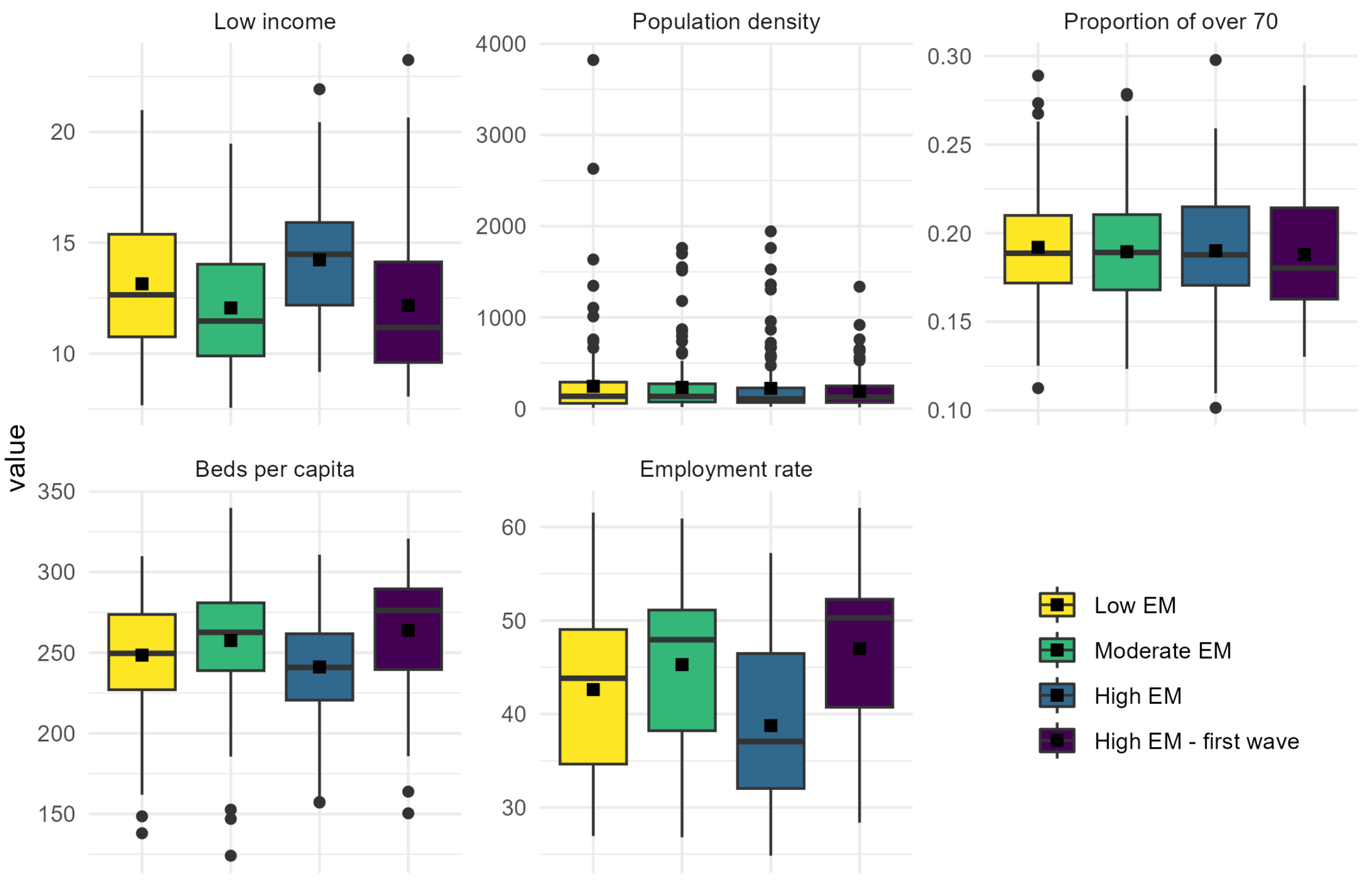
- Low-income: Frequency of residents with annual incomes between EUR 0 and 10.000. The variable was chosen to represent the poverty level of each LMA. Characterising LMAs as disadvantaged economic areas (or not disadvantaged) may enable us to understand whether a poor environment can be associated with positive EM. Source: Italian Revenue Agency, year 2019.
- Population density. Number of residents per km. The variable is widely recognised as correlated with infections. Source: ISTAT, year 2011.
- Proportion of over 70: Age is a high-risk factor at the individual level. At the macro level, it may help to understand whether an ageing population structure is also associated with positive EM. Source: ISTAT, year 2021.
- Beds per capita: The indicator includes beds for acute patients in the ordinary regime. Each value represents the number of beds per 100,000 inhabitants, including LMAs within a radius of 80 km from each site. That considers the catchment area of a large hospital hub to be wider than the LMA in which it is located. The variable is a proxy of the health system’s local preparedness for the epidemic emergency immediately before the pandemic outbreak. Rough data source: Ministry of Health, year 2019.
- Employment rate: The employment rate tentatively highlighted possible connections between positive EM and the intensity of working activity. Source: ISTAT, year 2019.
2.2. EM Estimation
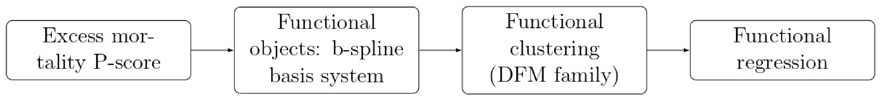
2.3. Two-Stage Statistical Analysis
2.3.1. Clustering Model
2.3.2. Functional Regression Model
3. Results
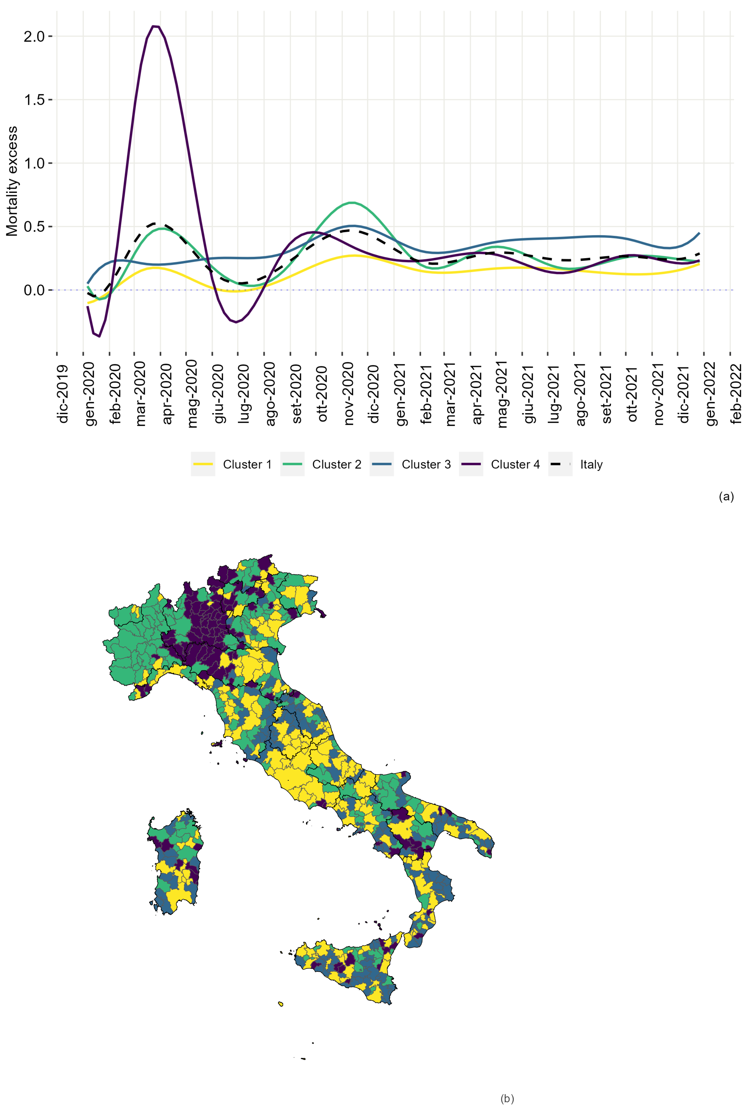
3.1. Clustering
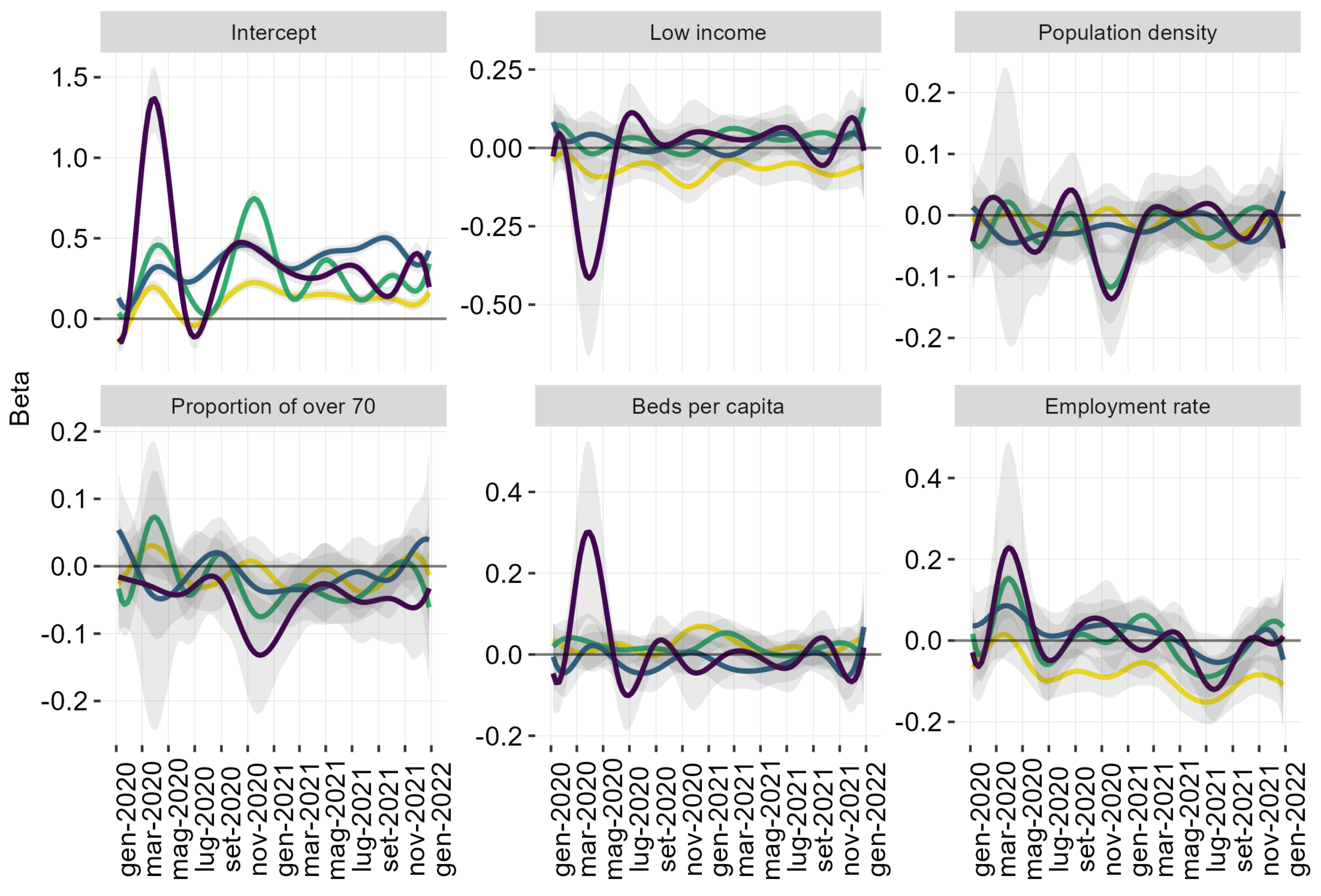
3.2. Functional Regression Models
3.2.1. Intercept
3.2.2. Low-Income
3.2.3. Population Density
3.2.4. Proportion of over 70
3.2.5. Beds Per Capita
3.2.6. Employment Rate
4. Discussion
Limitations and Future Developments
5. Conclusions
Supplementary Materials
Author Contributions
Funding
Institutional Review Board Statement
Informed Consent Statement
Data Availability Statement
Conflicts of Interest
Abbreviations
| EM | Excess Mortality |
| LMAs | Labour Market Areas |
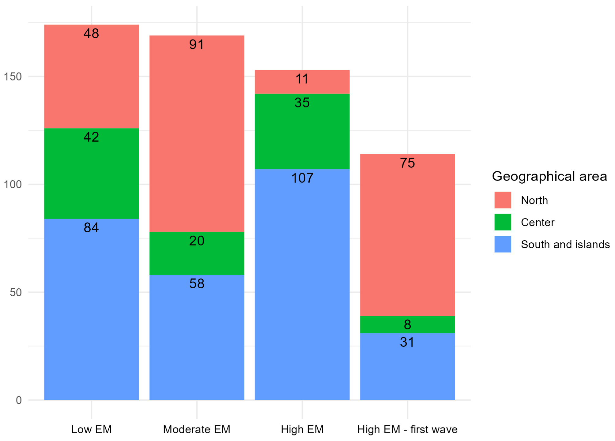
Appendix A. Clusters Description


Appendix B. Formalization of Clusters’ Models

| Cov. Matrix | Definition |
|---|---|
| not diagonal and different between clusters | |
| not diagonal and common between clusters | |
| diagonal and different between and within clusters | |
| diagonal, common within clusters and different between clusters | |
| diagonal, different within clusters and common between clusters | |
| diagonal and common between and within clusters | |
| diagonal different between clusters | |
| diagonal common between clusters |
References
- Riccardo, F.; Ajelli, M.; Andrianou, X.D.; Bella, A.; Del Manso, M.; Fabiani, M.; Bellino, S.; Boros, S.; Urdiales, A.M.; Marziano, V.; et al. Epidemiological characteristics of COVID-19 cases and estimates of the reproductive numbers 1 month into the epidemic, Italy, 28 January to 31 March 2020. Eurosurveillance 2020, 25, 2000790. [Google Scholar] [CrossRef] [PubMed]
- Dati Della Sorveglianza Integrata COVID-19 in Italia. Available online: https://www.epicentro.iss.it/coronavirus/sars-cov-2-dashboard (accessed on 1 February 2022).
- Beaney, T.; Clarke, J.M.; Jain, V.; Golestaneh, A.K.; Lyons, G.; Salman, D.; Majeed, A. Excess mortality: The gold standard in measuring the impact of COVID-19 worldwide? J. R. Soc. Med. 2020, 113, 329–334. [Google Scholar] [CrossRef] [PubMed]
- Blangiardo, M.; Cameletti, M.; Pirani, M.; Corsetti, G.; Battaglini, M.; Baio, G. Estimating weekly excess mortality at sub-national level in Italy during the COVID-19 pandemic. PLoS ONE 2020, 15, e0240286. [Google Scholar] [CrossRef]
- Maruotti, A.; Jona-Lasinio, G.; Divino, F.; Lovison, G.; Ciccozzi, M.; Farcomeni, A. Estimating COVID-19-induced excess mortality in Lombardy, Italy. Aging Clin. Exp. Res. 2022, 34, 475–479. [Google Scholar] [CrossRef] [PubMed]
- Ceccarelli, E.; Dorrucci, M.; Minelli, G.; Jona Lasinio, G.; Prati, S.; Battaglini, M.; Corsetti, G.; Bella, A.; Boros, S.; Petrone, D.; et al. Assessing COVID-19-Related Excess Mortality Using Multiple Approaches—Italy, 2020–2021. Int. J. Environ. Res. Public Health 2022, 19, 16. [Google Scholar] [CrossRef]
- Dorrucci, M.; Minelli, G.; Boros, S.; Manno, V.; Prati, S.; Battaglini, M.; Corsetti, G.; Andrianou, X.; Riccardo, F.; Fabiani, M.; et al. Excess mortality in Italy during the COVID-19 pandemic: Assessing the differences between the first and the second wave, year 2020. Front. Public Health 2021, 16, 927. [Google Scholar] [CrossRef]
- Achilleos, S.; Quattrocchi, A.; Gabel, J.; Heraclides, A.; Kolokotroni, O.; Constantinou, C.; Pagola Ugarte, M.; Nicolaou, N.; Rodriguez-Llanes, J.M.; Bennett, C.M.; et al. Excess all-cause mortality and COVID-19-related mortality: A temporal analysis in 22 countries, from January until August 2020. Int. J. Epidemiol. 2022, 51, 35–53. [Google Scholar] [CrossRef]
- Modig, K.; Ahlbom, A.; Ebeling, M. Excess mortality from COVID-19: Weekly excess death rates by age and sex for Sweden and its most affected region. Eur. J. Public Health 2021, 31, 17–22. [Google Scholar] [CrossRef]
- Vanella, P.; Basellini, U.; Lange, B. Assessing excess mortality in times of pandemics based on principal component analysis of weekly mortality data—The case of COVID-19. Genus 2021, 77, 16. [Google Scholar] [CrossRef]
- Gibertoni, D.; Adja, K.Y.C.; Golinelli, D.; Reno, C.; Regazzi, L.; Lenzi, J.; Sanmarchi, F.; Fantini, M.P. Patterns of COVID-19 related excess mortality in the municipalities of Northern Italy during the first wave of the pandemic. Health Place 2021, 67, 102508. [Google Scholar] [CrossRef]
- Stang, A.; Standl, F.; Kowall, B.; Brune, B.; Böttcher, J.; Brinkmann, M.; Dittmer, U.; Jöckel, K.H. Excess mortality due to COVID-19 in Germany. J. Infect. 2020, 81, 797–801. [Google Scholar] [CrossRef]
- Aburto, J.M.; Schöley, J.; Kashnitsky, I.; Zhang, L.; Rahal, C.; Missov, T.I.; Mills, M.C.; Dowd, J.B.; Kashyap, R. Quantifying impacts of the COVID-19 pandemic through life-expectancy losses: A population-level study of 29 countries. Int. J. Epidemiol. 2022, 51, 63–74. [Google Scholar] [CrossRef]
- Cuéllar, L.; Torres, I.; Romero-Severson, E.; Mahesh, R.; Ortega, N.; Pungitore, S.; Hengartner, N.; Ke, R. Excess deaths reveal the true spatial, temporal and demographic impact of COVID-19 on mortality in Ecuador. Int. J. Epidemiol. 2022, 51, 54–62. [Google Scholar] [CrossRef]
- European Harmonised Labour Market Areas—Methodology on Functional Geographies with Potential. Available online: https://ec.europa.eu/eurostat/web/products-statistical-working-papers/product/-/asset_publisher/DuuxBAj0uSCB/content/ks-tc-20-002?_com_liferay_asset_publisher_web_portlet_AssetPublisherPortlet_INSTANCE_DuuxBAj0uSCB_assetEntryId=10992201&_co (accessed on 15 March 2022).
- Ascani, A.; Faggian, A.; Montresor, S. The geography of COVID-19 and the structure of local economies: The case of Italy. J. Reg. Sci. 2021, 61, 407–441. [Google Scholar] [CrossRef]
- Bernstein, C.N.; Kraut, A.; Blanchard, J.F.; Rawsthorne, P.; Yu, N.; Walld, R. The relationship between inflammatory bowel disease and socioeconomic variables. Am. J. Gastroenterol. 2001, 96, 2117–2125. [Google Scholar] [CrossRef]
- Cadum, E.; Costa, G.; Biggeri, A.; Martuzzi, M. Deprivazione e mortalità: Un indice di deprivazione per l’analisi delle disuguaglianze su base geografica. Epidemiol. Prev. 1999, 23, 175–187. [Google Scholar]
- Mansfield, E.R.; Helms, B.P. Detecting multicollinearity. Am. Stat. 1982, 36, 158–160. [Google Scholar]
- Composizione dei Sistemi Locali del Lavoro. Available online: https://www.istat.it/it/archivio/252261 (accessed on 1 February 2022).
- Aron, J.; Muellbauer, J.; Giattino, C.; Ritchie, H. A pandemic primer on excess mortality statistics and their comparability across countries. World Data 2020. [Google Scholar]
- ISTAT-ISS. Settimo Rapporto. Impatto dell’Epidemia COVID-19 Sulla Mortalità Totale Della Popolazione Residente; Istituto Nazionale di Statistica: Rome, Italy, 2022.
- WHO. Global Excess Deaths Associated with COVID-19: January 2020–December 2021; WHO: Geneva, Switzerland, 2022; Volume 1.
- Bouveyron, C.; Côme, E.; Jacques, J. The discriminative functional mixture model for a comparative analysis of bike sharing systems. Ann. Appl. Stat. 2015, 9, 1726–1760. [Google Scholar] [CrossRef]
- Morris, J.S. Functional regression. Annu. Rev. Stat. Appl. 2015, 2, 321–359. [Google Scholar] [CrossRef]
- Ramsay, J.; Hooker, G.; Graves, S. Introduction to functional data analysis. In Functional Data Analysis with R and MATLAB; Springer: Berlin/Heidelberg, Germany, 2009; pp. 1–19. [Google Scholar]
- Bouveyron, C.; Brunet, C. Simultaneous model-based clustering and visualization in the Fisher discriminative subspace. Stat. Comput. 2012, 22, 301–324. [Google Scholar] [CrossRef]
- Schwarz, G. Estimating the dimension of a model. Ann. Stat. 1978, 461–464. [Google Scholar] [CrossRef]
- Goldsmith, J.; Kitago, T. Assessing systematic effects of stroke on motor control by using hierarchical function-on-scalar regression. J. R. Stat. Soc. Ser. Appl. Stat. 2016, 65, 215–236. [Google Scholar] [CrossRef] [PubMed]
- Gelfand, A.E. Gibbs sampling. J. Am. Stat. Assoc. 2000, 95, 1300–1304. [Google Scholar] [CrossRef]
- Golinelli, D.; Lenzi, J.; Adja, K.Y.C.; Reno, C.; Sanmarchi, F.; Fantini, M.P.; Gibertoni, D. Small-scale spatial analysis shows the specular distribution of excess mortality between the first and second wave of the COVID-19 pandemic in Italy. Public Health 2021, 194, 182–184. [Google Scholar] [CrossRef]
- Michelozzi, P.; de’Donato, F.; Scortichini, M.; De Sario, M.; Noccioli, F.; Rossi, P.; Davoli, M. Mortality impacts of the coronavirus disease (COVID-19) outbreak by sex and age: Rapid mortality surveillance system, Italy, 1 February to 18 April 2020. Eurosurveillance 2020, 25, 2000620. [Google Scholar] [CrossRef]
- Scortichini, M.; Schneider dos Santos, R.; De’Donato, F.; De Sario, M.; Michelozzi, P.; Davoli, M.; Masselot, P.; Sera, F.; Gasparrini, A. Excess mortality during the COVID-19 outbreak in Italy: A two-stage interrupted time-series analysis. Int. J. Epidemiol. 2020, 49, 1909–1917. [Google Scholar] [CrossRef]
- DPCM Gazzetta Ufficiale Serie Generale, n. 62 del 09 Marzo 2020. Available online: https://www.gazzettaufficiale.it/eli/gu/2020/03/09/62/sg/pdf (accessed on 12 May 2022).
- DPCM Gazzetta Ufficiale, Serie Generale n 275 of 4 November 2020, Ordinary Supplement n.41. Available online: https://www.gazzettaufficiale.it/do/gazzetta/downloadPdf?dataPubblicazioneGazzetta=20201104&numeroGazzetta=275&tipoSerie=SG&tipoSupplemento=SO&numeroSupplemento=41&progressivo=0&numPagina=315&estensione=pdf&edizione=0&home= (accessed on 1 February 2022).
- Open Data su Consegna e Somministrazione dei Vaccini Anti COVID-19 in Italia—Commissario Straordinario per l’Emergenza COVID-19. Available online: https://github.com/italia/covid19-opendata-vaccini/blob/master/dati/somministrazioni-vaccini-latest.csv (accessed on 1 June 2022).
- Sacco, C.; Mateo-Urdiales, A.; Petrone, D.; Spuri, M.; Fabiani, M.; Vescio, M.F.; Bressi, M.; Riccardo, F.; Del Manso, M.; Bella, A.; et al. Estimating averted COVID-19 cases, hospitalisations, intensive care unit admissions and deaths by COVID-19 vaccination, Italy, January–September 2021. Eurosurveillance 2021, 26, 2101001. [Google Scholar] [CrossRef]
- ISTAT-ISS. Impatto Dell’Epidemia COVID-19 Sulla Mortalità Totale della Popolazione Residente; ANNO 2020 E Gennaio-Aprile 2021; Istituto Nazionale di Statistica: Rome, Italy, 2021. [Google Scholar]
- Primi Risultati Dell’Indagine di Sieroprevalenza sul SARS-CoV-2. Available online: https://www.istat.it/it/files//2020/08/ReportPrimiRisultatiIndagineSiero.pdf (accessed on 18 January 2023).
- Biggeri, A.; Saltelli, A. The Strange Numbers of COVID-19. Argumenta 2021, 7, 97–107. [Google Scholar]
- Evoluzione dei Sistemi Territoriali. 2007. Available online: https://www.istat.it/it/files//2014/12/Evoluzione-dei-sistemi-territoriali-2007.pdf (accessed on 25 August 2022).
- Gollwitzer, A.; Martel, C.; Brady, W.J.; Pärnamets, P.; Freedman, I.G.; Knowles, E.D.; Van Bavel, J.J. Partisan differences in physical distancing are linked to health outcomes during the COVID-19 pandemic. Nat. Hum. Behav. 2020, 4, 1186–1197. [Google Scholar] [CrossRef]
- Porcher, S.; Renault, T. Social distancing beliefs and human mobility: Evidence from Twitter. PLoS ONE 2021, 16, e0246949. [Google Scholar] [CrossRef]
- Walshe, N.; Fennelly, M.; Hellebust, S.; Wenger, J.; Sodeau, J.; Prentice, M.; Grice, C.; Jordan, V.; Comerford, J.; Downey, V.; et al. Assessment of Environmental and Occupational Risk Factors for the Mitigation and Containment of a COVID-19 Outbreak in a Meat Processing Plant. Front. Public Health 2021, 27, 1544. [Google Scholar] [CrossRef]
- Gianicolo, E.A.; Russo, A.; Büchler, B.; Taylor, K.; Stang, A.; Blettner, M. Gender specific excess mortality in Italy during the COVID-19 pandemic accounting for age. Eur. J. Epidemiol. 2021, 36, 213–218. [Google Scholar] [CrossRef]


Disclaimer/Publisher’s Note: The statements, opinions and data contained in all publications are solely those of the individual author(s) and contributor(s) and not of MDPI and/or the editor(s). MDPI and/or the editor(s) disclaim responsibility for any injury to people or property resulting from any ideas, methods, instructions or products referred to in the content. |
© 2023 by the authors. Licensee MDPI, Basel, Switzerland. This article is an open access article distributed under the terms and conditions of the Creative Commons Attribution (CC BY) license (https://creativecommons.org/licenses/by/4.0/).
Share and Cite
Ceccarelli, E.; Minelli, G.; Egidi, V.; Jona Lasinio, G. Assessment of Excess Mortality in Italy in 2020–2021 as a Function of Selected Macro-Factors. Int. J. Environ. Res. Public Health 2023, 20, 2812. https://doi.org/10.3390/ijerph20042812
Ceccarelli E, Minelli G, Egidi V, Jona Lasinio G. Assessment of Excess Mortality in Italy in 2020–2021 as a Function of Selected Macro-Factors. International Journal of Environmental Research and Public Health. 2023; 20(4):2812. https://doi.org/10.3390/ijerph20042812
Chicago/Turabian StyleCeccarelli, Emiliano, Giada Minelli, Viviana Egidi, and Giovanna Jona Lasinio. 2023. "Assessment of Excess Mortality in Italy in 2020–2021 as a Function of Selected Macro-Factors" International Journal of Environmental Research and Public Health 20, no. 4: 2812. https://doi.org/10.3390/ijerph20042812
APA StyleCeccarelli, E., Minelli, G., Egidi, V., & Jona Lasinio, G. (2023). Assessment of Excess Mortality in Italy in 2020–2021 as a Function of Selected Macro-Factors. International Journal of Environmental Research and Public Health, 20(4), 2812. https://doi.org/10.3390/ijerph20042812