


Valuation of Ecosystem Services Based on EU Carbon Allowances—Optimal Recovery for a Coal Mining Area
 , , and
Abstract
1. Introduction
2. Materials and Methods
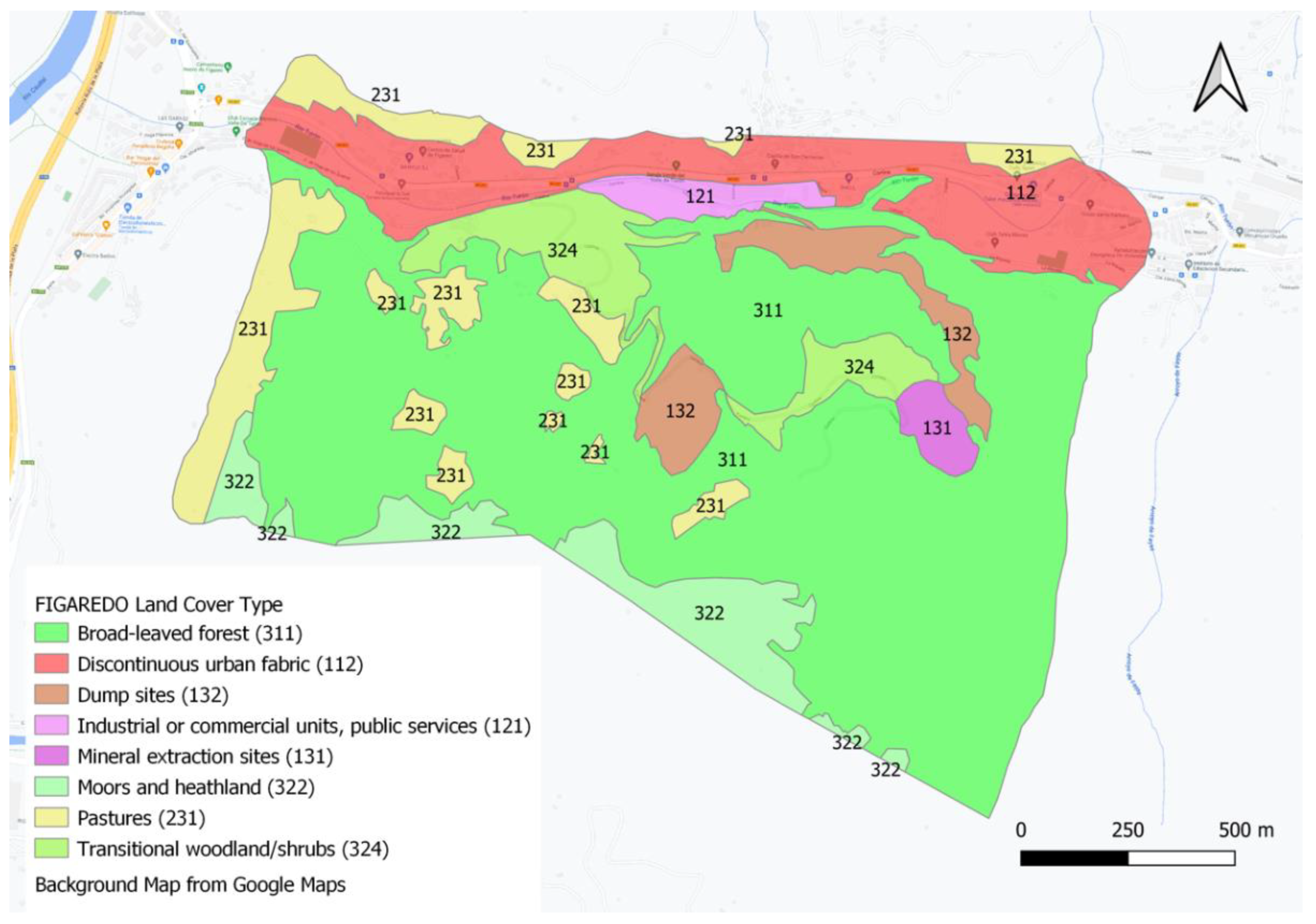
2.1. Study Area Description
2.2. Mapping of Relevant Ecosystems
2.3. Selection of Restoration Scenarios
2.4. Selection of Ecosystem Services
2.4.1. Provisioning Services: Fibre Production
2.4.2. Provisioning Services: Food Production
2.4.3. Regulating Services: Climate Regulation (Temperature)
2.4.4. Regulating Services: Climate Regulation (Humidity)
2.4.5. Regulating Services: Water Flow Regulation
2.4.6. Regulating Services: Erosion Control
2.4.7. Regulating Services: Air Purification
2.4.8. Regulating Services: Carbon Sequestration
2.4.9. Cultural Services: Qualities of Species or Ecosystems (Biodiversity)
2.5. Valuation Methodology
3. Results
3.1. Ecosystem Services Quantification
3.1.1. Provisioning Services: Fibre Production
3.1.2. Provisioning Services: Food Production
3.1.3. Regulating Services: Climate Regulation (Temperature)
3.1.4. Regulating Services: Climate Regulation (Humidity)
3.1.5. Regulating Services: Water Flow Regulation
3.1.6. Regulating Services: Erosion Control
3.1.7. Regulating Services: Air Purification
3.1.8. Regulating Services: Carbon Sequestration
3.1.9. Cultural Services: Qualities of Species or Ecosystems (Biodiversity)
3.2. Ecosystem Services Valuation
4. Discussion
5. Conclusions
Author Contributions
Funding
Institutional Review Board Statement
Informed Consent Statement
Data Availability Statement
Conflicts of Interest
References
- United Nations. Convention on Biological Diversity; United Nations: New York, NY, USA, 1992; Available online: https://www.cbd.int/doc/legal/cbd-en.pdf (accessed on 22 May 2021).
- De Groot, R.S.; Wilson, M.A.; Boumans, R.M.J. A typology for the classification, description and valuation of ecosystem functions, goods and services. Ecol. Econ. 2002, 41, 393–408. [Google Scholar] [CrossRef]
- Raudsepp-Hearne, C.; Peterson, G.D.; Bennett, E.M. Ecosystem service bundles for analysing trade-offs in diverse landscapes. Proc. Natl. Acad. Sci. USA 2010, 107, 5242–5247. [Google Scholar] [CrossRef] [PubMed]
- Baró, F.; Gómez-Baggethun, E.; Haase, D. Ecosystem service bundles along the urban-rural gradient: Insights for landscape planning and management. Ecosyst. Serv. 2017, 24, 147–159. [Google Scholar] [CrossRef]
- The Economics of Ecosystems and Biodiversity (TEEB). The Economics of Ecosystems and Biodiversity Ecological and Economic Foundations; Pushpam Kumar. Earthscan: London, UK; Washington, DC, USA, 2010; Available online: https://www.teebweb.org/wp-content/uploads/Study%20and%20Reports/Reports/Ecological%20and%20Economic%20Foundations/TEEB%20Ecological%20and%20Economic%20Foundations%20report/TEEB%20Foundations.pdf (accessed on 27 August 2022).
- Hein, L.; van Koppen, K.; de Groot, R.S.; van Ierland, E.C. Spatial Scales, Stakeholders and the Valuation of ecosystem services. Ecol. Econ. 2006, 57, 209–228. [Google Scholar] [CrossRef]
- Ahlroth, S.; Finnveden, G. Ecovalue08—A new valuation set for environmental systems analysis tools. J. Clean. Prod. 2011, 19, 1994–2003. [Google Scholar] [CrossRef]
- Gan, X.; Fernandez, I.; Guo, J.; Wilson, M.; Zhao, Y.; Zhou, B.; Wu, J. When to use what: Methods for weighting and aggregating sustainability indicators. Ecol. Indic. 2017, 81, 491–502. [Google Scholar] [CrossRef]
- Ahlroth, S.; Nilsson, M.; Finnveden, G.; Hjelm, O.; Hochschorner, E. Weighting and valuation in selected environmental systems analysis tools—Suggestions for further developments. J. Clean. Prod. 2011, 19, 145–156. [Google Scholar] [CrossRef]
- Zhao, C.; Liu, M.; Wang, K. Monetary valuation of the environmental benefits of green building: A case study of China. J. Clean. Prod. 2022, 365, 132704. [Google Scholar] [CrossRef]
- Damigos, D. An overview of environmental valuation methods for the mining industry. J. Clean. Prod. 2006, 14, 234–247. [Google Scholar] [CrossRef]
- Sijtsma, F.J.; van der Heide, C.M.; van Hinsberg, A. Beyond monetary measurement: How to evaluate projects and policies using the ecosystem services framework. Environ. Sci. Policy. 2013, 32, 14–25. [Google Scholar] [CrossRef]
- Wam, H.K.; Bunnefeld, N.; Clarke, N.; Hofstad, O. Conflicting interests of ecosystem services: Multi-criteria modelling and indirect evaluation of trade-offs between monetary and non-monetary measures. Ecosyst. Serv. 2016, 22, 280–288. [Google Scholar] [CrossRef]
- Saarikoski, H.; Mustajoki, J.; Barton, D.N.; Geneletti, D.; Langemeyer, J.; Gomez-Baggethun, E.; Marttunen, M.; Antunes, P.; Keune, H.; Santos, R. Multi-Criteria Decision Analysis and Cost-Benefit Analysis: Comparing alternative frameworks for integrated valuation of ecosystem services. Ecosyst. Serv. 2016, 22, 238–249. [Google Scholar] [CrossRef]
- Spangenberg, J.H.; Settele, J. Value pluralism and economic valuation—Defendable if well done. Ecosyst. Serv. 2016, 18, 100–109. [Google Scholar] [CrossRef]
- Bagstad, K.J.; Semmens, D.J.; Waage, S.; Winthrop, R. A comparative assessment of decision-support tools for ecosystem services quantification and valuation. Ecosyst. Serv. 2013, 5, 27–39. [Google Scholar] [CrossRef]
- Kang, N.; Hou, L.; Huang, J.; Liu, H. Ecosystem services valuation in China: A meta-analysis. Sci. Total Environ. 2022, 809, 151122. [Google Scholar] [CrossRef]
- Zhang, X.; Lu, X. Multiple criteria evaluation of ecosystem services for the Ruoergai Plateau Marshes in southwest China. Ecol. Econ. 2010, 69, 1463–1470. [Google Scholar] [CrossRef]
- Xie, G.; Zhang, C.; Zhen, L.; Zhang, L. Dynamic changes in the value of China’s ecosystem services. Ecosyst. Serv. 2017, 26, 146–154. [Google Scholar] [CrossRef]
- Larondelle, N.; Frantzeskaki, N.; Haase, D. Mapping transition potential with stakeholder- and policy-driven scenarios in Rotterdam City. Ecol. Indic. 2016, 70, 630–643. [Google Scholar] [CrossRef]
- Salo, A.A.; Hämäläinen, R.P. Preference programming through approximate ratio comparisons. Eur. J. Oper. Res. 1995, 82, 458–475. [Google Scholar] [CrossRef]
- European Union. EU Emissions Trading System Handbook; European Commission: Brussels, Belgium, 2015; Available online: https://ec.europa.eu/clima/system/files/2017-03/ets_handbook_en.pdf (accessed on 27 August 2022).
- RECOVERY Project. Recovery of Degraded and Transformed Ecosystems in Coal Mining-Affected Areas; Contract No. 847205, 2019; European Commission, Research Fund for Coal and Steel (RFCS): Brussels, Belgium, 2019; Available online: www.recoveryproject.eu (accessed on 23 September 2022).
- Haines-Young, R.; Potschin, M.B. Common International Classification of Ecosystem Services (CICES) V5.1 and Guidance on the Application of the Revised Structure; European Environment Agency: Copenhagen, Denmark, 2018; Available online: www.cices.eu (accessed on 2 September 2022).
- Larondelle, N.; Haase, D. Valuing post-mining landscapes using an ecosystem services approach—An example from Germany. Ecol. Indic. 2012, 18, 567–574. [Google Scholar] [CrossRef]
- Kain, J.H.; Larondelle, N.; Haase, D.; Kaczorowska, A. Exploring local consequences of two land-use alternatives for the supply of urban ecosystem services in Stockholm year 2050. Ecol. Indic. 2016, 70, 615–629. [Google Scholar] [CrossRef]
- URBES Project. European Urban Biodiversity and Ecosystem Services; Biodiversa Network & The Swedish Research Council Formas: Gothenburg, Sweden, 2012; Available online: https://www.biodiversa.org/121 (accessed on 28 October 2022).
- Burkhard, B.; Kroll, F.; Müller, F.; Windhorst, W. Landscapes’ capacities to provide ecosystem services—A concept for land-cover based assessments. Landsc. Online 2009, 15, 1–22. [Google Scholar] [CrossRef]
- Schwarz, N.; Bauer, A.; Haase, D. Assessing climate impacts of planning policies-An estimation for the urban region of Leipzig (Germany). Environ. Impact Assess. Rev. 2011, 31, 97–111. [Google Scholar] [CrossRef]
- Nunes, A.N.; de Almeida, A.C.; Coelho, C.O.A. Impacts of land use and cover type on runoff and soil erosion in a marginal area of Portugal. Appl. Geogr. 2011, 31, 687–699. [Google Scholar] [CrossRef]
- Jones, L.; Vieno, M.; Morton, D.; Cryle, P.; Holland, M.; Carnell, E.; Nemitz, E.; Hall, J.; Beck, R.; Reis, S.; et al. Developing Estimates for the Valuation of Air Pollution Removal in Ecosystem Accounts; Final Report for the Office of National Statistics, United Nations; Centre for Ecology and Hydrology: Wallingford, UK, 2017; Available online: https://nora.nerc.ac.uk/id/eprint/524081/7/N524081RE.pdf (accessed on 28 October 2022).
- Strohbach, M.W.; Haase, D. Above-ground carbon storage by urban trees in Leipzig, Germany: Analysis of patterns in a European city. Landsc. Urban Plan. 2012, 104, 95–104. [Google Scholar] [CrossRef]
- Haase, D.; Haase, A.; Rink, D. Conceptualising the nexus between urban shrinkage and ecosystem services. Landsc. Urban Plan. 2014, 132, 159–169. [Google Scholar] [CrossRef]
- Martin, D.M.; Mazzota, M. Non-monetary valuation using Multi-Criteria Decision Analysis: Sensitivity of additive aggregation methods to scaling and compensation assumptions. Ecosyst. Serv. 2018, 29, 13–22. [Google Scholar] [CrossRef]
- Salo, A.A.; Hämäläinen, R.P. Preference Assessment by Imprecise Ratio Statements (PAIRS). Oper. Res. 1992, 40, 1053–1061. [Google Scholar] [CrossRef]
- Hämäläinen, R.P.; Helenius, J. WIMPRE: Workbench for Interactive Preference Programming; Helsinki University of Technology: Finland, Helsinky, 1998; Available online: https://sal.aalto.fi/en/resources/downloadables/winpre (accessed on 18 December 2021).
- Tanouchi, H.; Olsson, J.; Lindström, G.; Kawamura, A.; Amaguchi, H. Improving Urban Runoff in Multi-Basin Hydrological Simulation by the HYPE Model Using EEA Urban Atlas: A Case Study in the Sege River Basin, Sweden. Hydrology 2019, 6, 28. [Google Scholar] [CrossRef]
- Cavard, X.; Macdonald, S.E.; Bergeron, Y.; Chen, H.Y.H. Importance of mixedwoods for biodiversity conservation: Evidence for understory plants, songbirds, soil fauna, and ectomycorrhizae in northern forests. Environ. Rev. 2011, 19, 142–161. [Google Scholar] [CrossRef]
- Ember Technologies, Inc. Daily EU ETS Carbon Market Price (Euros); Sandbag Climate Campaign CIC: England/Wales, UK, 2022; Available online: https://ember-climate.org/data/carbon-price-viewer (accessed on 27 September 2022).
- Harmsworth, C.; Jacoby, J. Managing Change Initiatives: Real and Simple; Trafford Publishing: Bloomington, IN, USA, 2015. [Google Scholar]
- EU Carbon Permits. Available online: https://tradingeconomics.com/commodity/carbon (accessed on 15 October 2022).


| Item | EUR/m2 | EUR/ha |
|---|---|---|
| Tree plantation (250 trees/ha) | 0.170 | 1700 |
| Clearing and cleaning/year | 0.045 | 450 |
| Slow-release fertiliser/year | 0.020 | 200 |
| Watering/year | 0.013 | 130 |
| CLC Classes | Thermal Emissivity | Evapotranspiration Potential | Runoff | |||
|---|---|---|---|---|---|---|
| Emission | Index | f | Index | % Rainfall | Index | |
| Discontinuous urban fabric (112) | 139.4 | 3.5 | 0.9 | 2.8 | 65.0 | 1.0 |
| Industry or commercial units (121) | 141.5 | 1.0 | 0.8 | 1 | 65.0 | 1.0 |
| Mineral extraction sites (131) | 137.0 | 6.4 | 1.0 | 4.6 | 12.3 | 8.3 |
| Dump sites (132) | 139.0 | 4.0 | 1.0 | 4.6 | 12.3 | 8.3 |
| Pastures (231) | 135.4 | 8.3 | 1.1 | 6.4 | 0.6 | 9.9 |
| Broad-leaved forest (311) | 134.0 | 10.0 | 1.1 | 6.4 | 0.1 | 10.0 |
| Coniferous forest (312) | 137.4 | 5.9 | 1.3 | 10 | 6.2 | 9.2 |
| Moors and heathland (322) | 137.0 | 6.4 | 1.1 | 6.4 | 12.3 | 8.3 |
| Transitional woodland/shrub (324) | 136.0 | 7.6 | 1.1 | 6.4 | 0.2 | 10.0 |
| CLC Classes | Soil Erosion | Dry Deposition of Pollutants | Above-Ground Carbon Storage | |||
|---|---|---|---|---|---|---|
| g/m2 | Index | k/year | Index | t C/ha | Index | |
| Discontinuous urban fabric (112) | 193.0 | 6.9 | 2.02 | 1.0 | 20.0 | 3.6 |
| Industry or commercial units (121) | 193.0 | 6.9 | 2.02 | 1.0 | 8.52 | 2.1 |
| Mineral extraction sites (131) | 551.3 | 1.0 | 2.02 | 1.0 | ≈0 | 1.0 |
| Dump sites (132) | 551.3 | 1.0 | 2.02 | 1.0 | ≈0 | 1.0 |
| Pastures (231) | 2.4 | 10.0 | 149.4 | 6.2 | ≈0 | 1.0 |
| Broad-leaved forest (311) | 1.4 | 10.0 | 258.9 | 10.0 | 68.31 | 10.0 |
| Coniferous forest (312) | 15.6 | 9.6 | 258.9 | 10.0 | ≈0 | 1.0 |
| Moors and heathland (322) | 29.8 | 9.1 | 120.2 | 5.1 | 4.0 | 1.5 |
| Transitional woodland/shrub (324) | 1.2 | 10.0 | 189.6 | 7.6 | 10.12 | 2.3 |
| CLC Classes | Impact | Index |
|---|---|---|
| Discontinuous urban fabric (112) | 0 | 1 |
| Industry or commercial units (121) | 0 | 1 |
| Mineral extraction sites (131) | 1 | 4 |
| Dump sites (132) | 1 | 4 |
| Pastures (231) | 2 | 7 |
| Broad-leaved forest (311) | 3 | 10 |
| Coniferous forest (312) | 2 | 7 |
| Moors and heathland (322) | 2.5 | 8.5 |
| Transitional woodland/shrub (324) | 2.5 | 8.5 |
| Ecosystem Service | Indicator | Quantification Method |
|---|---|---|
| Fibre production | Forest productivity | m3/ha/year |
| Food production | Livestock production | units/ha/year |
| Climate regulation (Temperature) | Land surface thermal emissions | Thermal emissivity |
| Climate regulation (Humidity) | Evapotranspiration | Evapotranspiration potential |
| Water flow regulation | Runoff | Runoff in % of total rainfall |
| Erosion control | Soil loss | Soil erosion in g/m2 during a monitored period |
| Air purification | Pollutant capture | Dry deposition of pollutants in t/year |
| Carbon sequestration | Carbon storage | Above-ground carbon storage in t/ha |
| Qualities of species or ecosystems (Biodiversity) | Impact of shrinkage- related cover patterns | Degree of suitability |
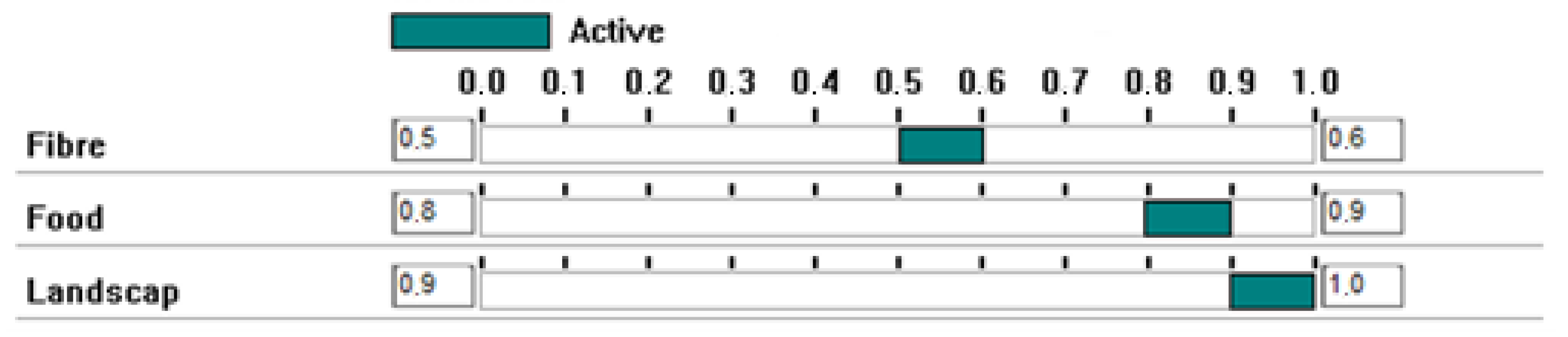
| Scenarios | Lower Bound | Mean | Upper Bound |
|---|---|---|---|
| Landscape | 0.87 | 0.93 | 0.99 |
| Fibre | 0.49 | 0.60 | 0.71 |
| Food | 0.47 | 0.57 | 0.67 |
| Attribute/Ecosystem Service | Comparative Average Weight * | Value per ha |
|---|---|---|
| Temperature | 25% | EUR 1567 |
| Waterflow | 20% | EUR 1235 |
| Erosion | 15% | EUR 940 |
| Air purification | 40% | EUR 2507 |
| Carbon sequestration | 60% | EUR 3760 |
| Humidity | 15% | EUR 940 |
| Biodiversity | 100% | EUR 6267 |
| Total | EUR 17,216 |
| Scenarios | Highest Ecosystem Service Contribution | Interval Means | Ecosystem Services Values | NPVs | Total Values |
|---|---|---|---|---|---|
| Landscape | EUR 17,216 | 0.93 | EUR 16,011 | EUR –5486 | EUR 10,525 |
| Fibre | EUR 17,216 | 0.60 | EUR 10,330 | EUR 2386 | EUR 12,716 |
| Food | EUR 17,216 | 0.57 | EUR 9813 | EUR 3323 | EUR 13,136 |
| Scenarios | Highest Ecosystem Service Contribution | Interval Means | Ecosystem Services Values | NPVs | Total Values |
|---|---|---|---|---|---|
| Landscape | EUR 47,570 | 0.93 | EUR 44,240 | EUR −5486 | EUR 38,754 |
| Fibre | EUR 47,570 | 0.60 | EUR 28,542 | EUR 2386 | EUR 30,928 |
| Food | EUR 47,570 | 0.57 | EUR 27,115 | EUR 3323 | EUR 30,438 |
Disclaimer/Publisher’s Note: The statements, opinions and data contained in all publications are solely those of the individual author(s) and contributor(s) and not of MDPI and/or the editor(s). MDPI and/or the editor(s) disclaim responsibility for any injury to people or property resulting from any ideas, methods, instructions or products referred to in the content. |
© 2022 by the authors. Licensee MDPI, Basel, Switzerland. This article is an open access article distributed under the terms and conditions of the Creative Commons Attribution (CC BY) license (https://creativecommons.org/licenses/by/4.0/).
Share and Cite
Krzemień, A.; Álvarez Fernández, J.J.; Riesgo Fernández, P.; Fidalgo Valverde, G.; Garcia-Cortes, S. Valuation of Ecosystem Services Based on EU Carbon Allowances—Optimal Recovery for a Coal Mining Area. Int. J. Environ. Res. Public Health 2023, 20, 381. https://doi.org/10.3390/ijerph20010381
Krzemień A, Álvarez Fernández JJ, Riesgo Fernández P, Fidalgo Valverde G, Garcia-Cortes S. Valuation of Ecosystem Services Based on EU Carbon Allowances—Optimal Recovery for a Coal Mining Area. International Journal of Environmental Research and Public Health. 2023; 20(1):381. https://doi.org/10.3390/ijerph20010381
Chicago/Turabian StyleKrzemień, Alicja, Juan José Álvarez Fernández, Pedro Riesgo Fernández, Gregorio Fidalgo Valverde, and Silverio Garcia-Cortes. 2023. "Valuation of Ecosystem Services Based on EU Carbon Allowances—Optimal Recovery for a Coal Mining Area" International Journal of Environmental Research and Public Health 20, no. 1: 381. https://doi.org/10.3390/ijerph20010381
APA StyleKrzemień, A., Álvarez Fernández, J. J., Riesgo Fernández, P., Fidalgo Valverde, G., & Garcia-Cortes, S. (2023). Valuation of Ecosystem Services Based on EU Carbon Allowances—Optimal Recovery for a Coal Mining Area. International Journal of Environmental Research and Public Health, 20(1), 381. https://doi.org/10.3390/ijerph20010381