
Temporal and Spatial Analysis of Alzheimer’s Disease Based on an Improved Convolutional Neural Network and a Resting-State FMRI Brain Functional Network

Abstract
1. Introduction
2. Materials and Methods
2.1. Data Selection
2.2. Image Preprocessing
2.3. Whole-Brain Functional Link Matrix FC
2.4. The Improved Method Proposed in This Paper
- (1)
- GAN based data augmentation
- (2)
- Spatial feature extraction based on CNNs
- (3)
- RNN
- (4)
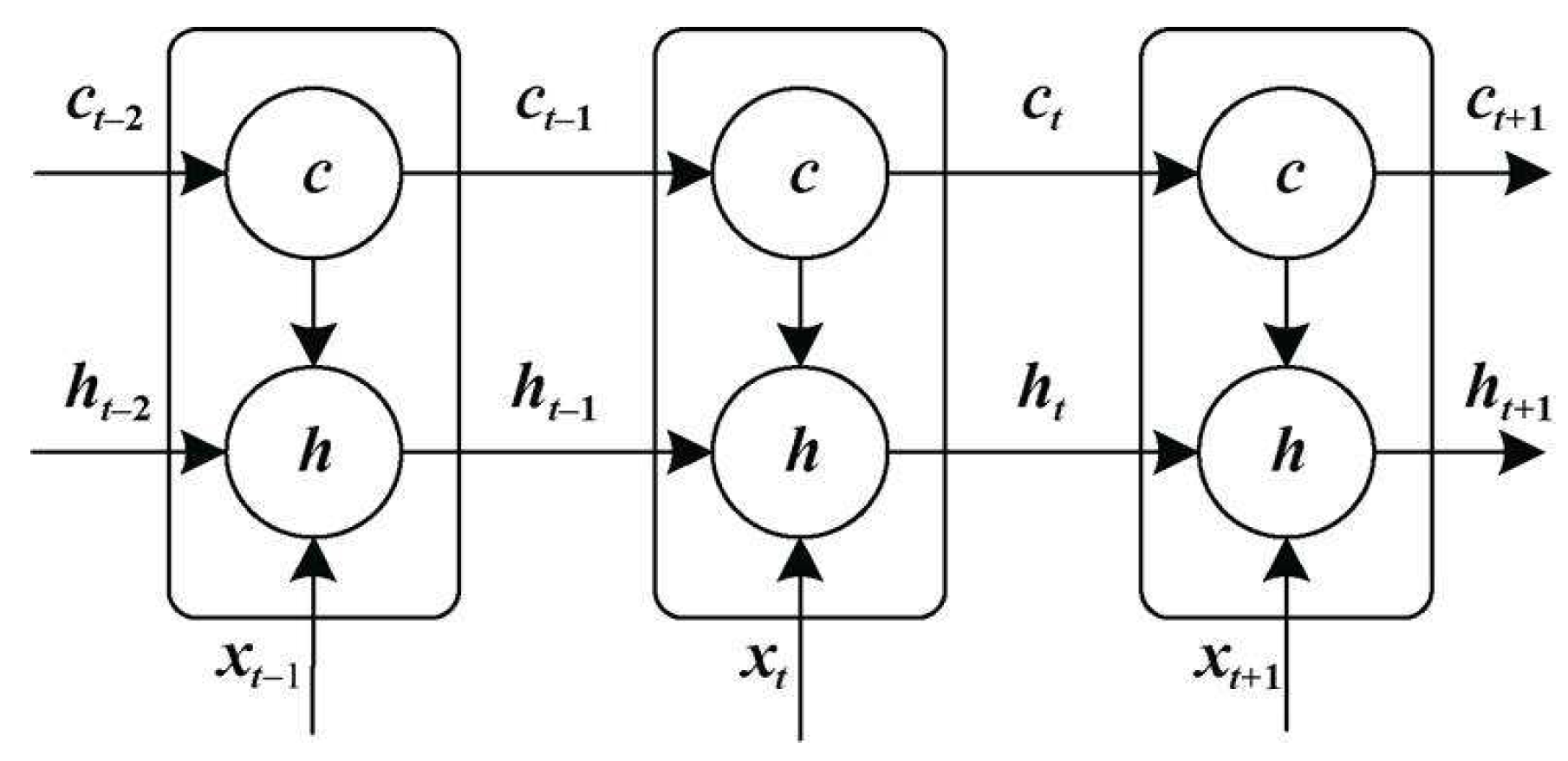
- LSTM
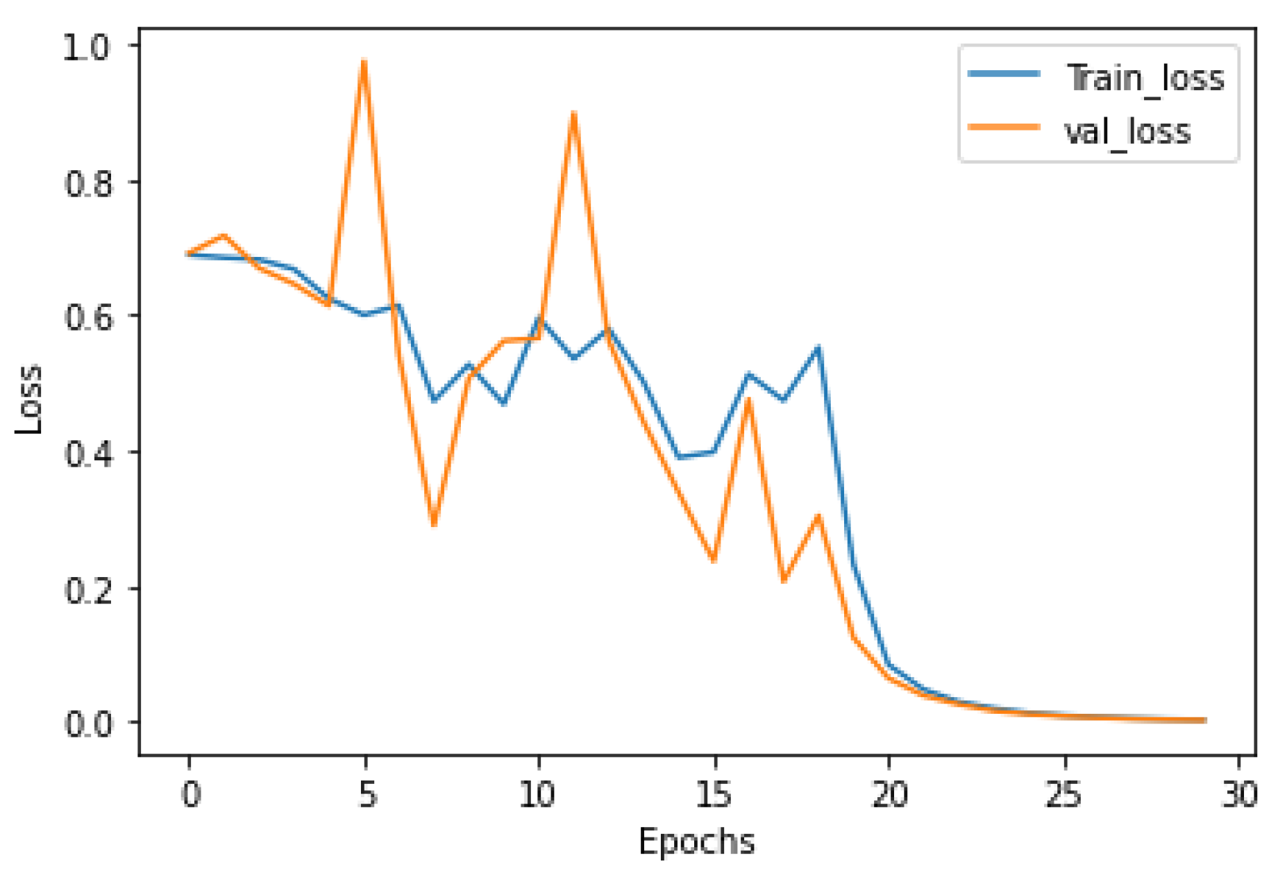
3. Experimental Result
4. Conclusions
Author Contributions
Funding
Institutional Review Board Statement
Informed Consent Statement
Data Availability Statement
Acknowledgments
Conflicts of Interest
References
- Ouyang, X.; Chen, K.; Yao, L.; Wu, X.; Zhang, J.; Li, K.; Jin, Z.; Guo, X. Independent Component Analysis-Based Identification of Covariance Patterns of Microstructural White Matter Damage in Alzheimer’s Disease. PLoS ONE 2015, 10, e0119714. [Google Scholar] [CrossRef] [PubMed]
- Anderson, N.D. State of the science on mild cognitive impairment (MCI). CNS Spectr. 2019, 24, 78–87. [Google Scholar] [CrossRef] [PubMed]
- Cheng, B.; Zhu, B.; Pu, S. Multi-auxiliary domain transfer learning for diagnosis of MCI conversion. Neurol. Sci. 2022, 43, 1721–1739. [Google Scholar] [CrossRef] [PubMed]
- Song, X.; Mao, M.; Qian, X. Auto-Metric Graph Neural Network Based on a Meta-Learning Strategy for the Diagnosis of Alzheimer’s Disease. IEEE J. Biomed. Health Inform. 2021, 25, 3141–3152. [Google Scholar] [CrossRef]
- Li, H.; Habes, M.; Wolk, D.A.; Fan, Y. Alzheimer’s Disease Neuroimaging Initiative and the Australian Imaging Biomarkers and Lifestyle Study of Aging. A deep learning model for early prediction of Alzheimer’s disease dementia based on hippocampal magnetic resonance imaging data. Alzheimer’s Dement. 2019, 15, 1059–1070. [Google Scholar] [CrossRef]
- Ibrahim, B.; Suppiah, S.; Ibrahim, N.; Mohamad, M.; Hassan, H.A.; Nasser, N.S.; Saripan, M.I. Diagnostic power of resting-state fMRI for detection of network connectivity in Alzheimer’s disease and mild cognitive impairment: A systematic review. Hum. Brain Mapp. 2021, 42, 2941–2968. [Google Scholar] [CrossRef]
- Wang, J.; Wu, X.; Li, M. Microcanonical and Canonical Ensembles for fMRI Brain Networks in Alzheimer’s Disease. Entropy 2021, 23, 216. [Google Scholar] [CrossRef]
- Luo, Y.; Sun, T.; Ma, C.; Zhang, X.; Ji, Y.; Fu, X.; Ni, H. Alterations of Brain Networks in Alzheimer’s Disease and Mild Cognitive Impairment: A Resting State fMRI Study Based on a Population-specific Brain Template. Neuroscience 2021, 452, 192–207. [Google Scholar] [CrossRef]
- Zhang, X.; Hu, B.; Ma, X.; Xu, L. Resting-State Whole-Brain Functional Connectivity Networks for MCI Classification Using L2-Regularized Logistic Regression. IEEE Trans. Nanobiosci. 2015, 14, 237–247. [Google Scholar] [CrossRef]
- Taie, S.A.; Ghonaim, W. A new model for early diagnosis of Alzheimer’s disease based on BAT-SVM classifier. Bull. Electr. Eng. Inform. 2021, 10, 759–766. [Google Scholar] [CrossRef]
- Xu, M.; Sanz, D.L.; Garces, P.; Maestu, F.; Li, Q.; Pantazis, D. A Graph Gaussian Embedding Method for Predicting Alzheimer’s Disease Progression with MEG Brain Networks. IEEE Trans. Biomed. Eng. 2021, 68, 1579–1588. [Google Scholar] [CrossRef]
- Dennis, E.L.; Thompson, P.M. Functional Brain Connectivity Using fMRI in Aging and Alzheimer’s Disease. Neuropsychol. Rev. 2014, 24, 49–62. [Google Scholar] [CrossRef] [PubMed]
- Borchert, R.; Azevedo, T.; Badhwar, A.; Bernal, J.; Betts, M.; Bruffaerts, R.; Burkhart, M.C.; Dewachter, I.; Gellersen, H.M.; Low, A.; et al. Artificial intelligence for diagnosis and prognosis in neuroimaging for dementia; a systematic review. medRxiv 2021. [Google Scholar] [CrossRef]
- Lim, Y.Y.; Kong, J.; Maruff, P.; Jaeger, J.; Huang, E.; Ratti, E. Longitudinal Cognitive Decline in Patients With Mild Cognitive Impairment or Dementia Due to Alzheimer’s Disease. J. Prev. Alzheimer’s Dis. 2022, 9, 178–183. [Google Scholar] [CrossRef] [PubMed]
- Tufail, A.B.; Ma, Y.K.; Zhang, Q.N. Binary Classification of Alzheimer’s Disease Using sMRI Imaging Modality and Deep Learning. J. Digit. Imaging 2020, 33, 1073–1090. [Google Scholar] [CrossRef]
- Lin, Y.; Huang, K.; Xu, H.; Qiao, Z.; Cai, S.; Wang, Y.; Huang, L. Predicting the progression of mild cognitive impairment to Alzheimer’s disease by longitudinal magnetic resonance imaging-based dictionary learning. Clin. Neurophysiol. 2020, 131, 2429–2439. [Google Scholar] [CrossRef]
- Wang, Z.; Xin, J.; Wang, Z.; Yao, Y.; Zhao, Y.; Qian, W. Brain Functional Network Modeling and Analysis Based on FMRI: A systematic review. Cogn. Neurodyn. 2021, 15, 389–403. [Google Scholar] [CrossRef]
- Weng, J.C.; Huang, S.Y.; Lee, M.S.; Ho, M.C. Association between functional brain alterations and neuropsychological scales in male chronic smokers using resting-state fMRI. Psychopharmacology 2021, 238, 1387–1399. [Google Scholar] [CrossRef]
- Huang, H.; Ding, Z.; Mao, D.; Yuan, J.; Zhu, F.; Chen, S.; Xu, Y.; Lou, L.; Feng, X.; Qi, L.; et al. PreSurgMapp: A MATLAB Toolbox for Presurgical Mapping of Eloquent Functional Areas Based on Task-Related and Resting-State Functional MRI. Neuroinformatics. 2016, 14, 421–438. [Google Scholar] [CrossRef]
- Zhang, L. Bayesian nonparametric models for functional magnetic resonance imaging (fMRI) data. Proc. SPIE 2015, 7963, 843–845. [Google Scholar]
- Waal, H.D.; Stam, C.; Lansbergen, M. Functional brain network organization in Alzheimer’s disease. Alzheimer’s Dement. 2013, 9, 670. [Google Scholar] [CrossRef]
- Iqbal, M.S.; Ahmad, I.; Bin, L.; Khan, S.; Rodrigues, J.J.P.C. Deep learning recognition of diseased and normal cell representation. Trans. Emerg. Telecommun. Technol. 2020, 32, e4017. [Google Scholar] [CrossRef]
- Xia, M.; Wang, J.; He, Y. BrainNet Viewer: A Network Visualization Tool for Human Brain Connectomics. PLoS ONE 2013, 8, e68910. [Google Scholar]
- Wang, J.; Wang, X.; Xia, M.; Liao, X.; Evans, A.; He, Y. GRETNA: A graph theoretical network analysis toolbox for imaging connectomics. Front. Hum. Neurosci. 2015, 9, 386. [Google Scholar]
- Schumacher, J.; Thomas, A.J.; Peraza, L.R.; Firbank, M.; O’Brien, J.T.; Taylor, J.P. Functional connectivity of the nucleus basalis of Meynert in Lewy body dementia and Alzheimer’s disease. Int. Psychogeriatr. 2021, 33, 89–94. [Google Scholar] [CrossRef]
- Iqbal, M.S.; Ahmad, I.; Khan, T.; Khan, S.; Ahmad, M.; Wang, L. Recent Advances of Deep Learning in Biology. Deep Learn. for Unmanned Systems 2021, 984, 709–732. [Google Scholar]
- Tian, H.; Deng, S.; Wang, C. A novel method for prediction of paraffin deposit in sucker rod pumping system based on CNN indicator diagram feature deep learning. J. Pet. Sci. Eng. 2021, 206, 108986. [Google Scholar] [CrossRef]
- Wang, K.; Chen, J.; Song, Z. Deep Neural Network-Embedded Stochastic Nonlinear State-Space Models and Their Applications to Process Monitoring. IEEE Trans. Neural Netw. Learn. Syst. 2021, 99, 1–13. [Google Scholar] [CrossRef]
- Won, J.; Callow, D.D.; Pena, G.S.; Jordan, L.S.; Arnold-Nedimala, N.A.; Nielson, K.A.; Smith, J.C. Hippocampal Functional Connectivity and Memory Performance After Exercise Intervention in Older Adults with Mild Cognitive Impairment. J. Alzheimer’s Dis. 2021, 82, 1015–1031. [Google Scholar] [CrossRef]
- Lyu, Q.; Xia, D.; Liu, Y.; Yang, X.; Li, R. Pyramidal convolution attention generative adversarial network with data augmentation for image denoising. Soft Comput. 2021, 25, 9273–9284. [Google Scholar] [CrossRef]
- Kattenborn, T.; Leitloff, J.; Schiefer, F.; Hinz, S. Review on Convolutional Neural Networks (CNN) in vegetation remote sensing. ISPRS 2021, 173, 24–49. [Google Scholar] [CrossRef]
- Iqbal, M.S.; Luo, B.; Mehmood, R.; Alrige, M.A.; Alharbey, R. Mitochondrial organelle movement classification (fission and fusion) via convolutional neural network approach. IEEE Access 2019, 7, 86570–86577. [Google Scholar] [CrossRef]
- Iqbal, M.S.; El-Ashram, S.; Hussain, S.; Khan, T.; Huang, S.; Mehmood, R.; Luo, B. Efficient cell classification of mitochondrial images by using deep learning. J. Opt. 2019, 48, 113–122. [Google Scholar] [CrossRef]
- Bai, Q.; Zhou, J.; He, L. PG-RNN: Using Position-gated Recurrent Neural Networks for Aspect-based Sentiment Classification. J Supercomput. 2022, 78, 4073–4094. [Google Scholar] [CrossRef]
- Rafi, S.H.; Masood, N.A.; Deeba, S.R. A Short-Term Load Forecasting Method Using Integrated CNN and LSTM Network. IEEE Access 2021, 9, 32436–32448. [Google Scholar] [CrossRef]
- Shao, X.; Kim, C.S. Multi-Step Short-Term Power Consumption Forecasting Using Multi-Channel LSTM With Time Location Considering Customer Behavior. IEEE Access 2020, 8, 125263–125273. [Google Scholar] [CrossRef]
- Livieris, I.E.; Pintelas, E.; Pintelas, P. A CNN–LSTM model for gold price time-series forecasting. Neural Comput. Appl. 2020, 32, 17351–17360. [Google Scholar] [CrossRef]
- Lei, B.; Yu, S.; Zhao, X.; Frangi, A.F.; Tan, E.-L.; ElAzab, A.; Wang, T.; Wang, S. Diagnosis of early Alzheimer’s disease based on dynamic high order networks. Brain Imaging Behav. 2021, 15, 276–287. [Google Scholar] [CrossRef]
- Cassady, K.E.; Adams, J.N.; Chen, X.; Maass, A.; Harrison, T.M.; Landau, S.; Baker, S.; Jagust, W. Alzheimer’s Pathology Is Associated with Dedifferentiation of Intrinsic Functional Memory Networks in Aging. Cereb Cortex. 2021, 31, 4781–4793. [Google Scholar] [CrossRef]
- Varone, G.; Boulila, W.; Giudice, M.L.; Benjdira, B.; Mammone, N.; Ieracitano, C.; Dashtipour, K.; Neri, S.; Gasparini, S.; Morabito, F.C.; et al. A Machine Learning Approach Involving Functional Connectivity Features to Classify Rest-EEG Psychogenic Non-Epileptic Seizures from Healthy Controls. Sensors 2021, 22, 129. [Google Scholar] [CrossRef]


| Classified | Samples | Sex (Male/Female) | Mean Age | MMSE | CDR |
|---|---|---|---|---|---|
| NC-bl | 100 | 50/50 | 70.80 | 29.56 | 0.02 |
| NC-12 m | 29.30 | 0.05 | |||
| NC-24 m | 29.62 | 0.08 | |||
| sMCI-bl | 75 | 37/38 | 72.56 | 27.56 | 0.50 |
| sMCI-12 m | 26.96 | 0.52 | |||
| sMCI-24 m | 25.55 | 0.62 | |||
| pMCI-bl | 72 | 32/40 | 75.60 | 26.52 | 0.85 |
| pMCI-12 m | 24.26 | 1.22 | |||
| pMCI-24 m | 22.98 | 2.36 | |||
| AD-bl | 65 | 30/35 | 78.20 | 23.35 | 3.26 |
| AD-12 m | 21.26 | 3.51 | |||
| AD-24 m | 18.75 | 3.95 |
| BL | Methods | Time | Accuracy (%) | Precision (%) | Recall (%) |
|---|---|---|---|---|---|
| NC VS. AD | SVM | BL | 86.1 | 83.9 | 80.0 |
| 12 m | 87.3 | 85.5 | 81.5 | ||
| 24 m | 88.5 | 84.4 | 83.1 | ||
| CNN | BL | 88.5 | 85.9 | 84.6 | |
| 12 m | 89.7 | 87.5 | 86.2 | ||
| 24 m | 91.0 | 89.1 | 87.7 | ||
| CNN + LSTM | BL | 90.3 | 88.9 | 86.2 | |
| 12 m | 91.0 | 87.9 | 89.2 | ||
| 24 m | 93.3 | 91.0 | 92.3 | ||
| sMCI VS. pMCI | SVM | BL | 68.0 | 66.7 | 69.4 |
| 12 m | 69.4 | 68.0 | 70.8 | ||
| 24 m | 70.1 | 68.4 | 72.2 | ||
| CNN | BL | 71.4 | 69.7 | 73.6 | |
| 12 m | 72.1 | 70.1 | 75.0 | ||
| 24 m | 73.5 | 71.4 | 76.4 | ||
| CNN + LSTM | BL | 74.1 | 72.4 | 76.4 | |
| 12 m | 74.8 | 72.7 | 77.8 | ||
| 24 m | 75.5 | 73.1 | 79.2 |
Publisher’s Note: MDPI stays neutral with regard to jurisdictional claims in published maps and institutional affiliations. |
© 2022 by the authors. Licensee MDPI, Basel, Switzerland. This article is an open access article distributed under the terms and conditions of the Creative Commons Attribution (CC BY) license (https://creativecommons.org/licenses/by/4.0/).
Share and Cite
Sun, H.; Wang, A.; He, S. Temporal and Spatial Analysis of Alzheimer’s Disease Based on an Improved Convolutional Neural Network and a Resting-State FMRI Brain Functional Network. Int. J. Environ. Res. Public Health 2022, 19, 4508. https://doi.org/10.3390/ijerph19084508
Sun H, Wang A, He S. Temporal and Spatial Analysis of Alzheimer’s Disease Based on an Improved Convolutional Neural Network and a Resting-State FMRI Brain Functional Network. International Journal of Environmental Research and Public Health. 2022; 19(8):4508. https://doi.org/10.3390/ijerph19084508
Chicago/Turabian StyleSun, Haijing, Anna Wang, and Shanshan He. 2022. "Temporal and Spatial Analysis of Alzheimer’s Disease Based on an Improved Convolutional Neural Network and a Resting-State FMRI Brain Functional Network" International Journal of Environmental Research and Public Health 19, no. 8: 4508. https://doi.org/10.3390/ijerph19084508
APA StyleSun, H., Wang, A., & He, S. (2022). Temporal and Spatial Analysis of Alzheimer’s Disease Based on an Improved Convolutional Neural Network and a Resting-State FMRI Brain Functional Network. International Journal of Environmental Research and Public Health, 19(8), 4508. https://doi.org/10.3390/ijerph19084508