
Assessing Trauma Center Accessibility for Healthcare Equity Using an Anti-Covering Approach


Abstract
:1. Introduction
2. Background
2.1. Inequality in Accessibility to Healthcare Services
2.2. Travel Time Distance Constraint and Commonly Covered Service Area
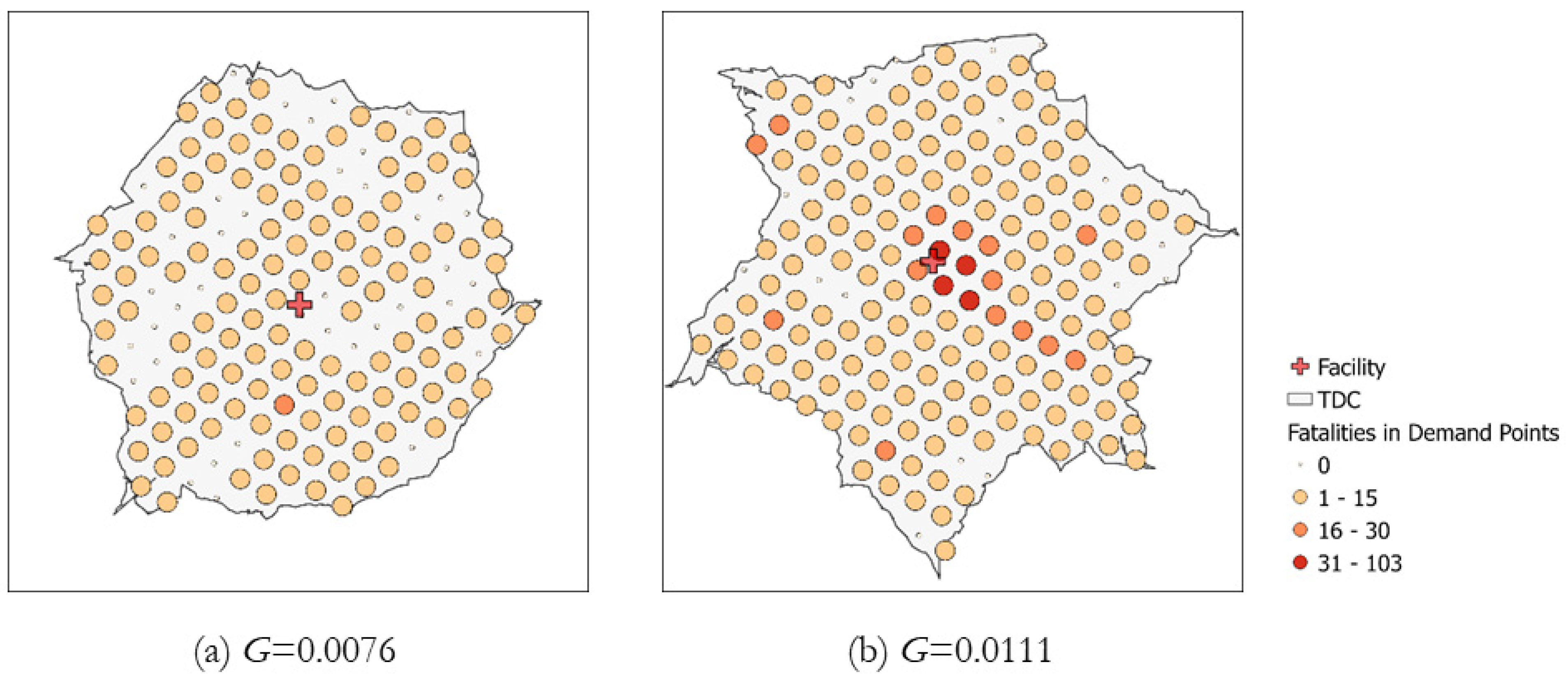
2.3. Spatially Autocorrelated Pattern of Demands
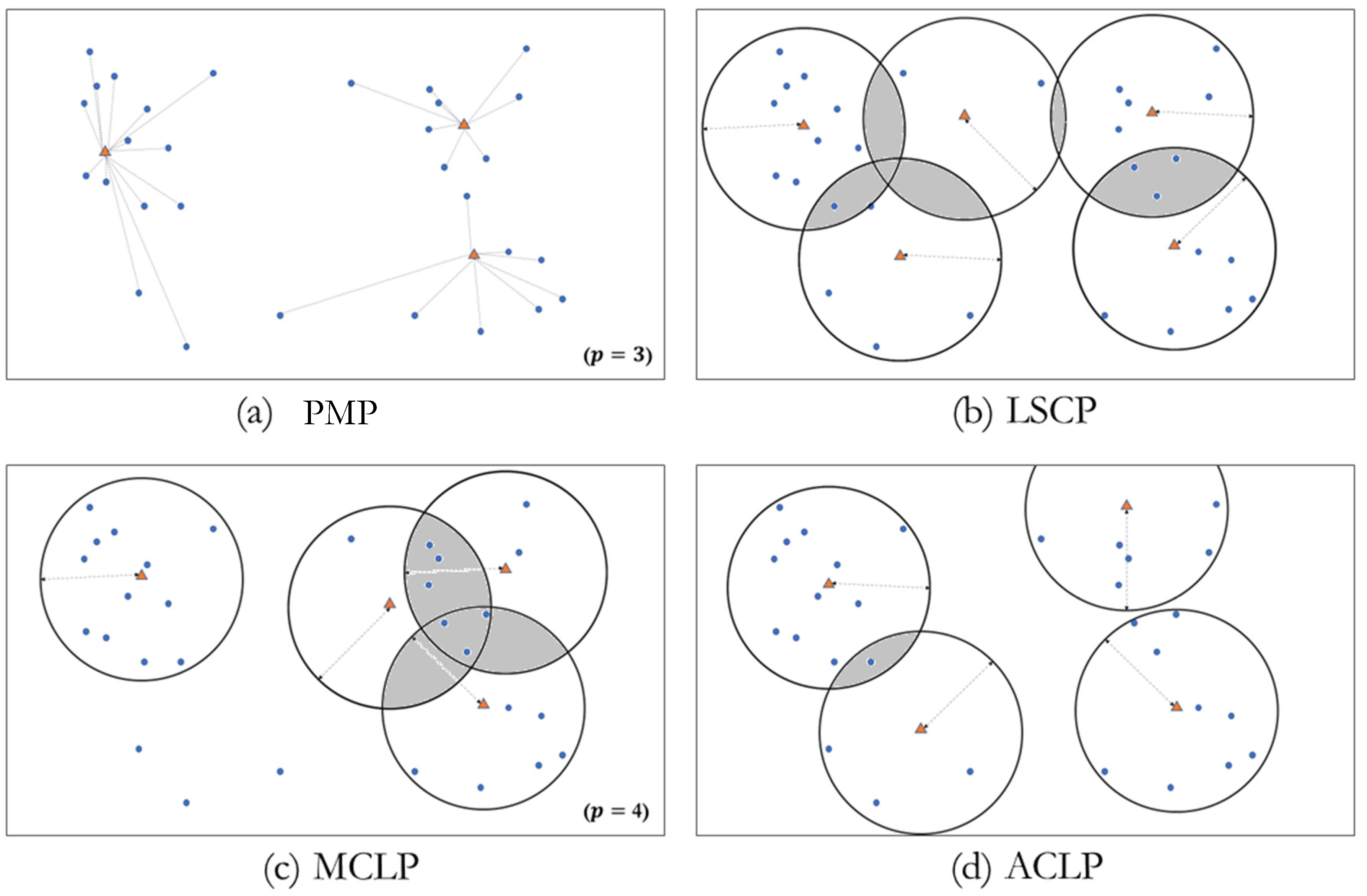
2.4. Locating Trauma Centers Using ACLP
3. Data
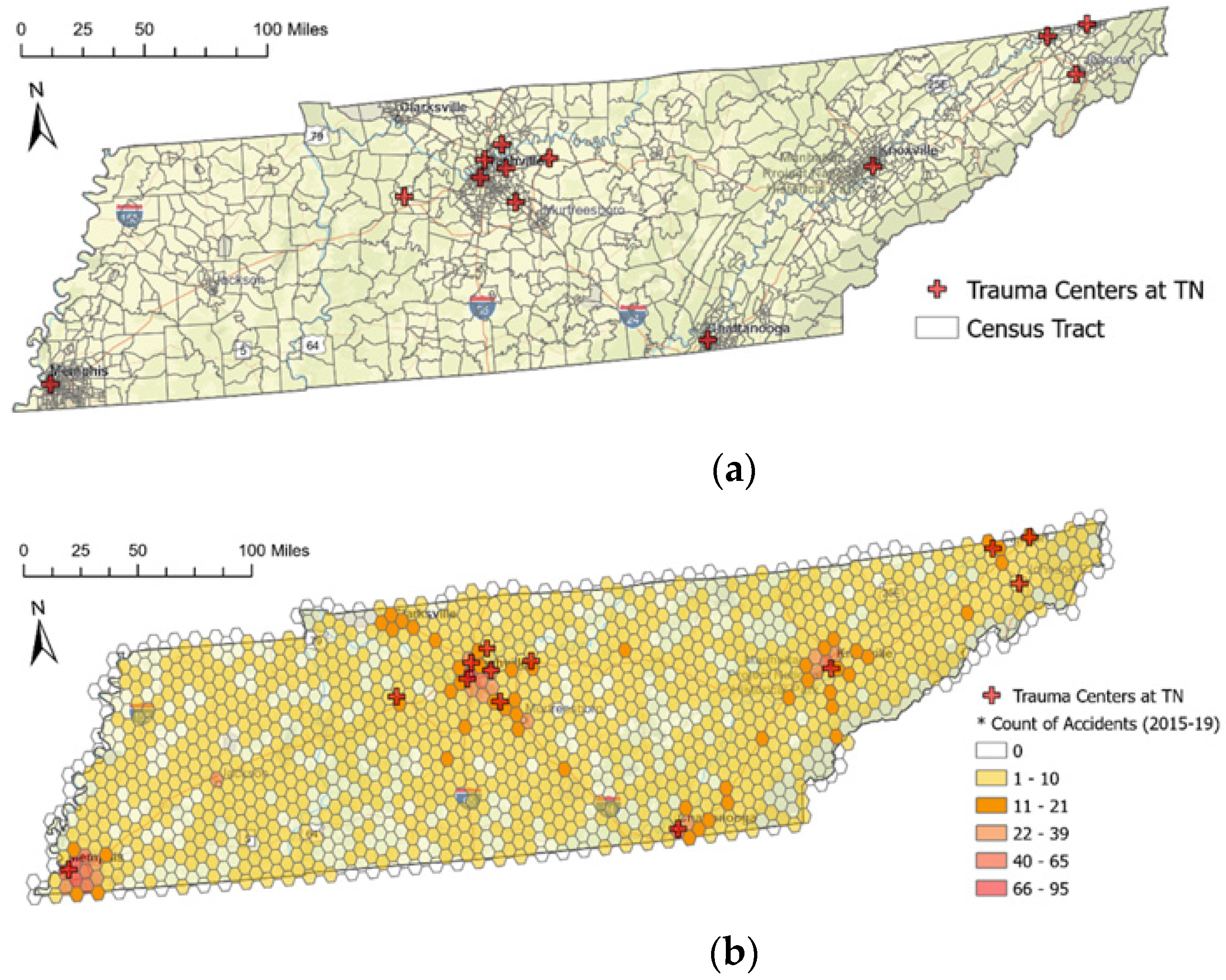
3.1. Trauma Centers and General Hospitals in Tennessee
3.2. Potential Demands
3.3. Tessellation of the Spatial Unit
3.4. Defining TDCs for Analysis
4. Methods
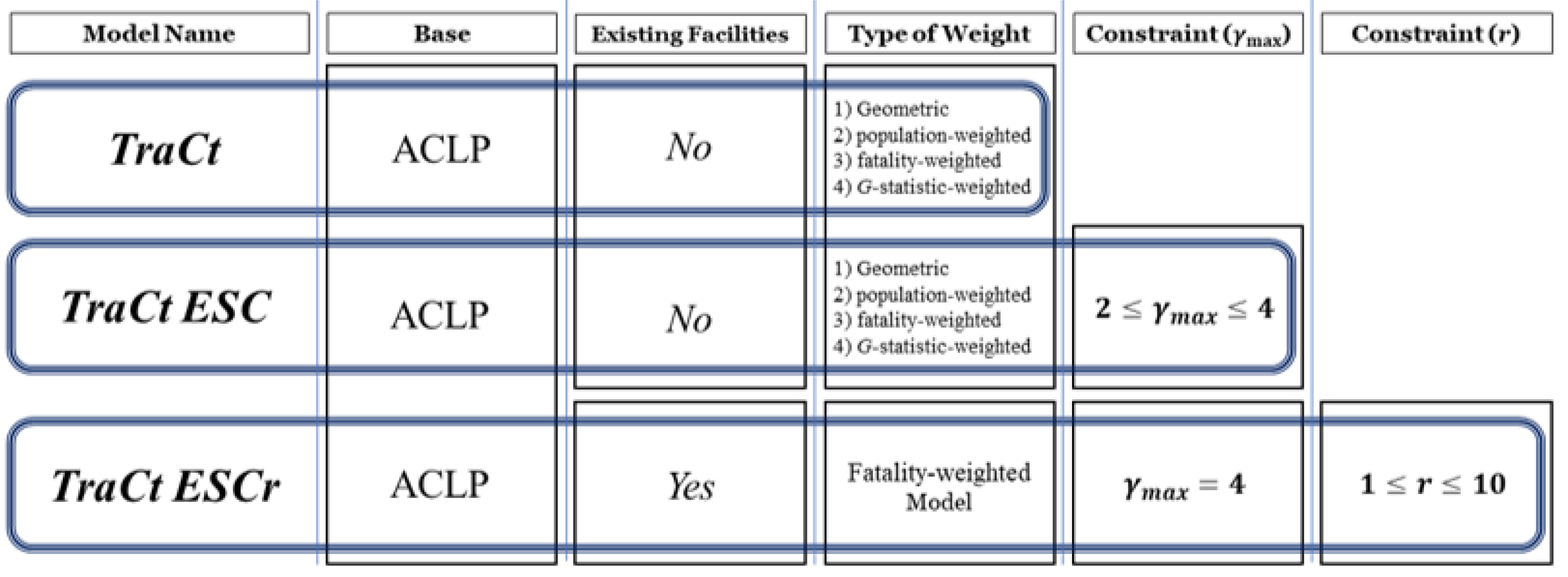
4.1. TraCt Model
4.2. TraCt-ESC Model
4.3. TraCt-ESCr Model
5. Results
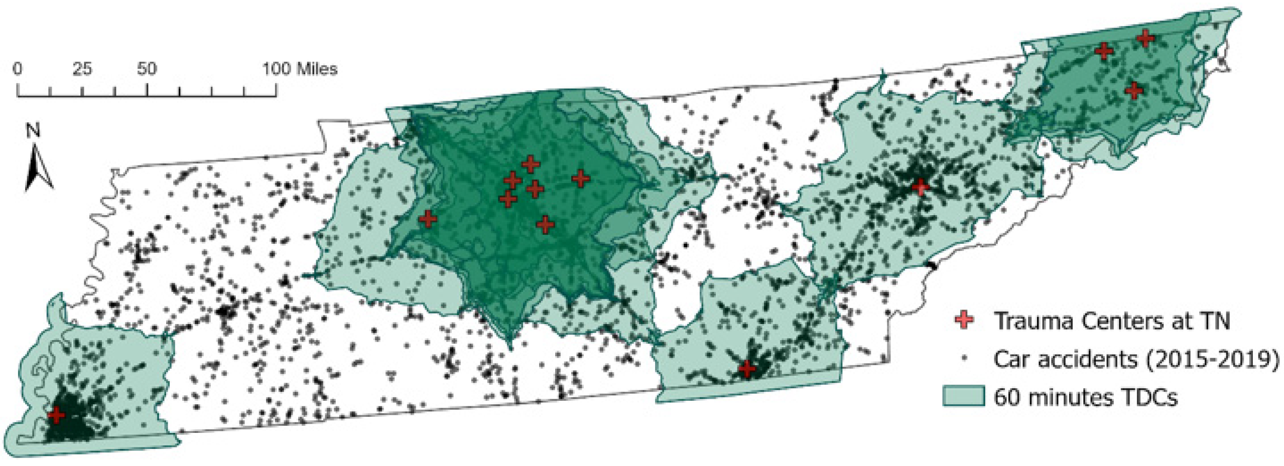
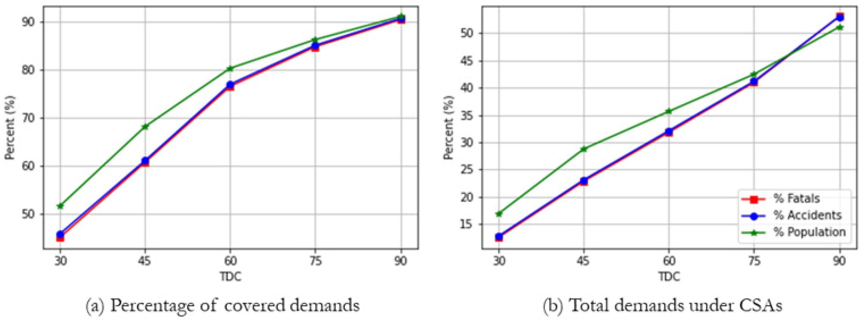
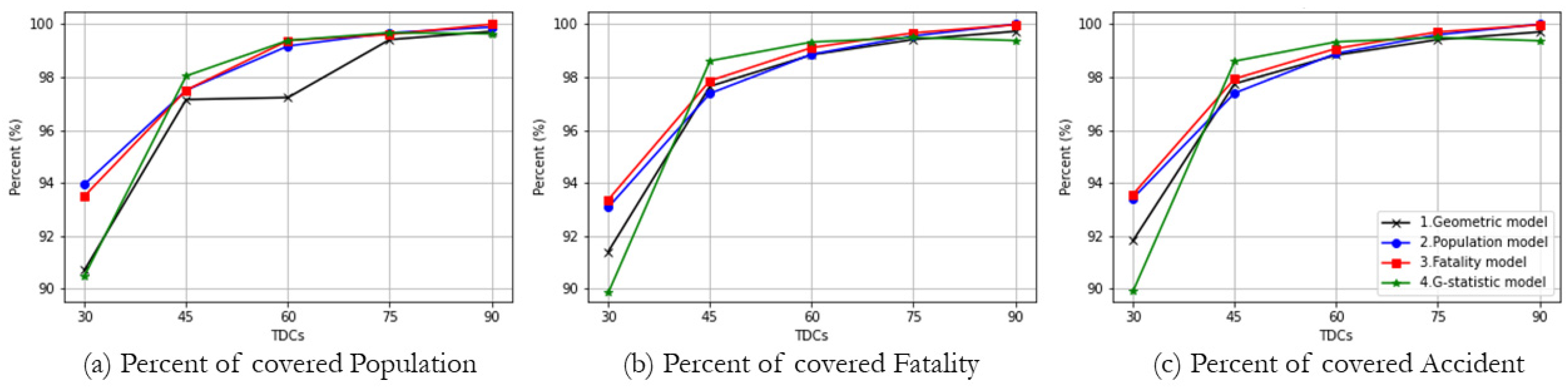
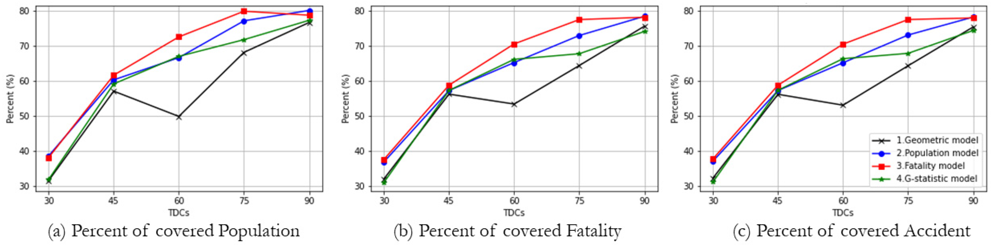
5.1. Demands Covered by Trauma Centers in Tennessee
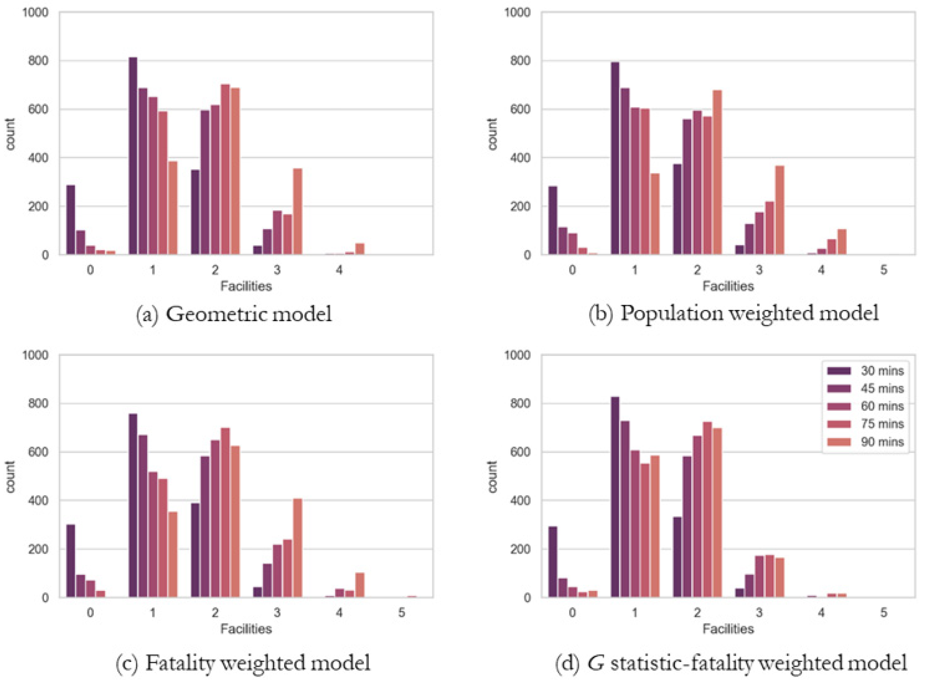
5.2. TraCt Model Solutions by Types of Weights
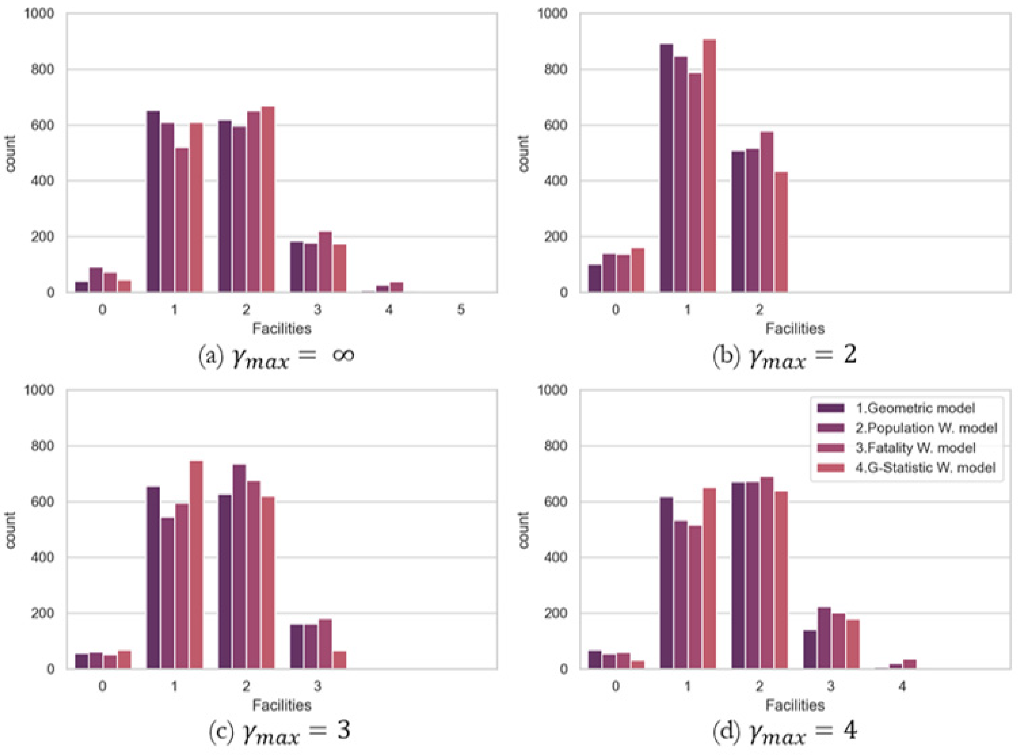
5.3. TraCt-ESC Model Solutions by Maximum Number of Accessible Facilities
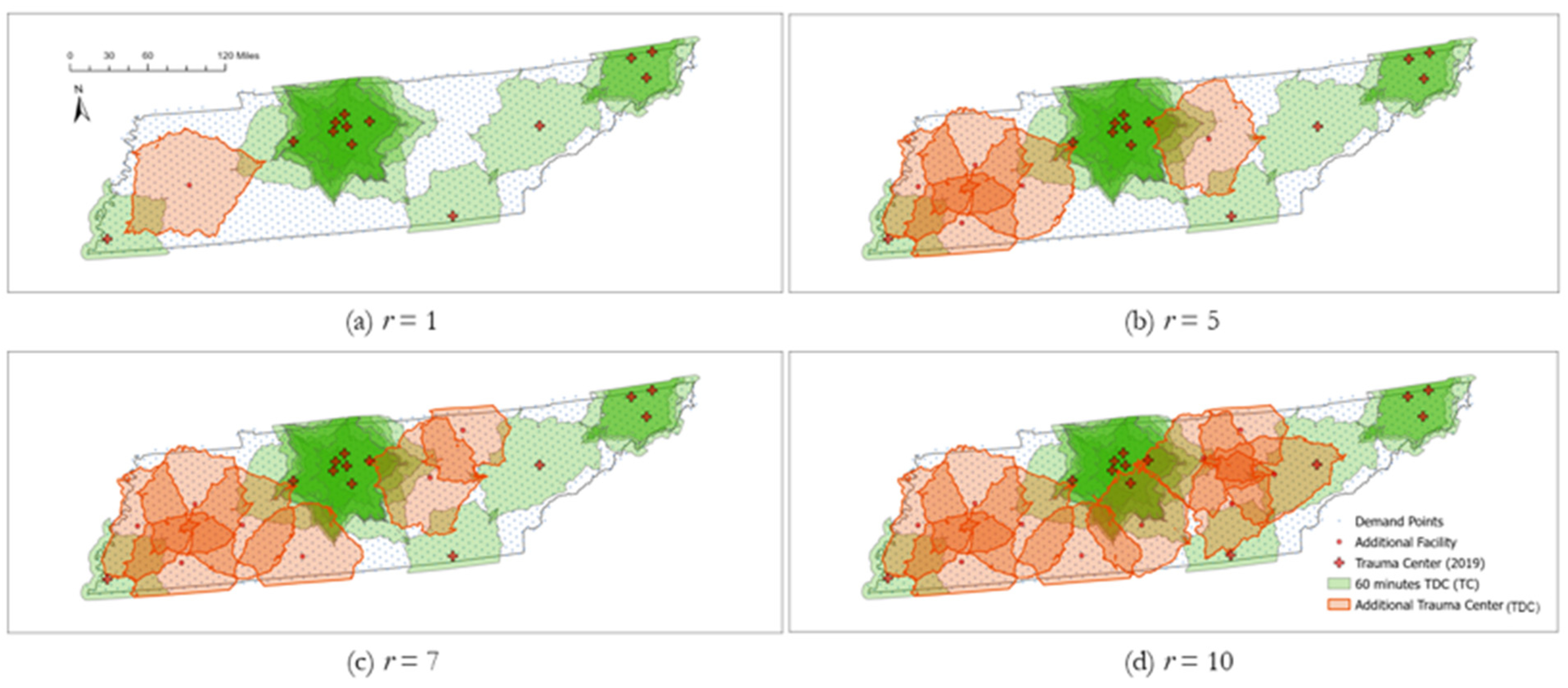
5.4. TraCt-ESCr Model Solutions by Number of Planned Facilities along with Current Trauma Centers
6. Conclusions
Author Contributions
Funding
Institutional Review Board Statement
Informed Consent Statement
Data Availability Statement
Conflicts of Interest
References
- Branas, C.C.; MacKenzie, E.J.; Williams, J.C.; Schwab, C.W.; Teter, H.M.; Flanigan, M.C.; ReVelle, C.S. Access to trauma centers in the United States. JAMA 2005, 293, 2626–2633. [Google Scholar] [CrossRef] [PubMed] [Green Version]
- Nathens, A.B.; Jurkovich, G.J.; Cummings, P.; Rivara, F.P.; Maier, R.V. The effect of organized systems of trauma care on motor vehicle crash mortality. JAMA 2000, 283, 1990–1994. [Google Scholar] [CrossRef] [PubMed] [Green Version]
- Nathens, A.B.; Jurkovich, G.J.; Rivara, F.P.; Maier, R.V. Effectiveness of state trauma systems in reducing injury-related mortality: A national evaluation. J. Trauma Acute Care Surg. 2000, 48, 25–30. [Google Scholar] [CrossRef] [PubMed]
- Thomas, S.H.; Harrison, T.H.; Buras, W.R.; Ahmed, W.; Cheema, F.; Wedel, S.K. Helicopter transport and blunt trauma mortality: A multicenter trial. J. Trauma 2002, 52, 136–145. [Google Scholar] [CrossRef] [PubMed]
- Hashmi, Z.G.; Jarman, M.P.; Uribe-Leitz, T.; Goralnick, E.; Newgard, C.D.; Salim, A.; Haider, A.H. Access delayed is access denied: Relationship between access to trauma center care and pre-hospital death. J. Am. Coll. Surg. 2019, 228, 9–20. [Google Scholar] [CrossRef] [PubMed] [Green Version]
- Hashmi, Z.G.; Haut, E.R.; Efron, D.T.; Salim, A.; Cornwell, E.E., III; Haider, A.H. A target to achieve zero preventable trauma deaths through quality improvement. JAMA Surg. 2018, 153, 686–689. [Google Scholar] [CrossRef]
- Kwon, A.M.; Garbett, N.C.; Kloecker, G.H. Pooled preventable death rates in trauma patients: Meta analysis and systematic review since 1990. Eur. J. Trauma Emerg. Surg. 2014, 40, 279–285. [Google Scholar] [CrossRef]
- Luo, W.; Yao, J.; Mitchell, R.; Zhang, X. Spatiotemporal access to emergency medical services in Wuhan, China: Accounting for scene and transport time intervals. Int. J. Health Geogr. 2020, 19, 52. [Google Scholar] [CrossRef]
- Balamurugan, A.; Delongchamp, R.; Im, L.; Bates, J.; Mehta, J.L. Neighborhood and acute myocardial infarction mortality as related to the driving time to percutaneous coronary intervention-capable hospital. J. Am. Hear. Assoc. 2016, 5, e002378. [Google Scholar] [CrossRef] [Green Version]
- Hansen, C.M.; Wissenberg, M.; Weeke, P.; Ruwald, M.H.; Lamberts, M.; Lippert, F.K.; Gislason, G.H.; Nielsen, S.L.; Køber, L.; Torp-Pedersen, C.; et al. Automated external defibrillators inaccessible to more than half of nearby cardiac arrests in public locations during evening, nighttime, and weekends. Circulation 2013, 128, 2224–2231. [Google Scholar] [CrossRef]
- O’Keeffe, C.; Nicholl, J.; Turner, J.; Goodacre, S. Role of ambulance response times in the survival of patients with out-of-hospital cardiac arrest. Emerg. Med. J. 2011, 28, 703–706. [Google Scholar] [CrossRef] [Green Version]
- Sánchez-Mangas, R.; García-Ferrrer, A.; De Juan, A.; Arroyo, A.M. The probability of death in road traffic accidents. How important is a quick medical response? Accid. Anal. Prev. 2010, 42, 1048–1056. [Google Scholar] [CrossRef] [PubMed]
- Lateef, F.; Anantharaman, V. Delays in the EMS response to and the evacuation of patients in high-rise buildings in Singapore. Prehospital Emerg. Care 2000, 4, 327–332. [Google Scholar] [CrossRef] [PubMed]
- Lerner, E.B.; Moscati, R.M. The golden hour: Scientific fact or medical “urban legend”? Acad. Emerg. Med. 2001, 8, 758–760. [Google Scholar] [CrossRef] [PubMed]
- Vanderschuren, M.; McKune, D. Emergency care facility access in rural areas within the golden hour?: Western Cape case study. Int. J. Health Geogr. 2015, 14, 5. [Google Scholar] [CrossRef] [Green Version]
- Trauma Care Annual Report 2019. Available online: https://www.tn.gov/content/dam/tn/health/healthprofboards/ems/Trauma-Care-Annual-Report-2019.pdf (accessed on 9 January 2022).
- Carr, B.G.; Bowman, A.J.; Wolff, C.S.; Mullen, M.T.; Holena, D.N.; Branas, C.C.; Wiebe, D.J. Disparities in access to trauma care in the United States: A population-based analysis. Injury 2017, 48, 332–338. [Google Scholar] [CrossRef] [Green Version]
- Daskin, M.S.; Stern, E.H. A hierarchical objective set covering model for emergency medical service vehicle deployment. Transp. Sci. 1981, 15, 137–152. [Google Scholar] [CrossRef]
- Moon, I.D.; Chaundry, S.S. An analysis of network location problems with distance constraints. Manag. Sci. 1984, 30, 290–307. [Google Scholar] [CrossRef]
- Church, R.L.; Murray, A. Chapter 5: Anti-cover. In Location Covering Models: History, Applications and Advancements; Church, R.L., Murray, A., Eds.; Springer: Cham, Switzerland, 2018; pp. 107–130. [Google Scholar]
- Caldwell, J.T.; Ford, C.L.; Wallace, S.P.; Wang, M.C.; Takahashi, L.M. Intersection of living in a rural versus urban area and race/ethnicity in explaining access to health care in the United States. Am. J. Public Health 2016, 106, 1463–1469. [Google Scholar] [CrossRef]
- Caldwell, J.T.; Ford, C.L.; Wallace, S.P.; Wang, M.C.; Takahashi, L.M. Racial and ethnic residential segregation and access to health care in rural areas. Health Place 2017, 43, 104–112. [Google Scholar] [CrossRef] [Green Version]
- Hsia, R.Y.J.; Shen, Y.C. Rising closures of hospital trauma centers disproportionately burden vulnerable populations. Health Aff. 2011, 30, 1912–1920. [Google Scholar] [CrossRef] [PubMed] [Green Version]
- Tansley, G.; Stewart, B.; Zakariah, A.; Boateng, E.; Achena, C.; Lewis, D.; Mock, C. Population-level spatial access to prehospital care by the national ambulance service in Ghana. Prehospital Emerg. Care 2016, 20, 768–775. [Google Scholar] [CrossRef] [Green Version]
- Ahmed, S.; Adams, A.M.; Islam, R.; Hasan, S.M.; Panciera, R. Impact of traffic variability on geographic accessibility to 24/7 emergency healthcare for the urban poor: A GIS study in Dhaka, Bangladesh. PLoS ONE 2019, 14, e0222488. [Google Scholar] [CrossRef] [PubMed] [Green Version]
- Janosikova, L.; Jankovic, P.; Kvet, M.; Zajacova, F. Coverage versus response time objectives in ambulance location. Int. J. Health Geogr. 2021, 20, 1–16. [Google Scholar]
- Jaklič, T.K.; Kovač, J. The impact of demographic changes on the organization of emergency medical services: The case of Slovenia. Organizacija 2015, 48, 247–258. [Google Scholar] [CrossRef] [Green Version]
- Veser, A.; Sieber, F.; Groß, S.; Prückner, S. The demographic impact on the demand for emergency medical services in the urban and rural regions of Bavaria, 2012–2032. J. Public Health 2015, 23, 181–188. [Google Scholar] [CrossRef] [Green Version]
- Aringhieri, R.; Carello, G.; Morale, D. Supporting decision making to improve the performance of an Italian Emergency Medical Service. Ann. Oper. Res. 2016, 236, 131–148. [Google Scholar] [CrossRef]
- Lowthian, J.A.; Cameron, P.A.; Stoelwinder, J.U.; Curtis, A.; Currell, A.; Cooke, M.W.; McNeil, J.J. Increasing utilisation of emergency ambulances. Aust. Health Rev. 2011, 35, 63–69. [Google Scholar] [CrossRef] [Green Version]
- Nagata, T.; Takamori, A.; Kimura, Y.; Kimura, A.; Hashizume, M.; Nakahara, S. Trauma center accessibility for road traffic injuries in Hanoi, Vietnam. J. Trauma Manag. Outcomes 2011, 5, 11. [Google Scholar] [CrossRef] [Green Version]
- Pedigo, A.S.; Odoi, A. Investigation of disparities in geographic accessibility to emergency stroke and myocardial infarction care in East Tennessee using geographic information systems and network analysis. Ann. Epidemiol. 2010, 20, 924–930. [Google Scholar] [CrossRef]
- Busingye, D.; Pedigo, A.; Odoi, A. Temporal changes in geographic disparities in access to emergency heart attack and stroke care: Are we any better today? Spat. Spatio-Temporal. Epidemiol. 2011, 2, 247–263. [Google Scholar] [CrossRef] [PubMed]
- Golden, A.P.; Odoi, A. Emergency medical services transport delays for suspected stroke and myocardial infarction patients. BMC Emerg. Med. 2015, 15, 34. [Google Scholar] [CrossRef] [PubMed] [Green Version]
- Chen, W.; Wheeler, K.K.; Huang, Y.; Lin, S.M.; Sui, D.Z.; Xiang, H. Evaluation of spatial accessibility to Ohio trauma centers using a GIS-based gravity model. J. Adv. Med. Med. Res. 2015, 10, 1–10. [Google Scholar] [CrossRef]
- Tansley, G.; Schuurman, N.; Erdogan, M.; Bowes, M.; Green, R.; Asbridge, M.; Yanchar, N. Development of a model to quantify the accessibility of a Canadian trauma system. Can. J. Emerg. Med. 2017, 19, 285–292. [Google Scholar] [CrossRef] [Green Version]
- Wei, R.; Clay Mann, N.; Dai, M.; Hsia, R.Y. Injury-based Geographic Access to Trauma Centers. Acad. Emerg. Med. 2019, 26, 192–204. [Google Scholar] [CrossRef] [Green Version]
- Toregas, C.; Swain, R.; ReVelle, C.; Bergman, L. The location of emergency service facilities. Oper. Res. 1971, 19, 1363–1373. [Google Scholar] [CrossRef]
- Caccetta, L.; Dzator, M. Heuristic methods for locating emergency facilities. Proc. Modsim. 2005, 2005, 1744–1750. [Google Scholar]
- Murray, A.T.; Grubesic, T.H. Locational planning of health care facilities. In Spatial Analysis in Health Geography; Routledge: London, UK, 2016; pp. 265–282. [Google Scholar]
- Ye, H.; Kim, H. Locating healthcare facilities using a network-based covering location problem. GeoJournal 2016, 81, 875–890. [Google Scholar] [CrossRef]
- Baxt, W.G.; Moody, P. The impact of a rotorcraft aeromedical emergency care service on trauma mortality. JAMA 1983, 249, 3047–3051. [Google Scholar] [CrossRef]
- Getis, A.; Ord, J.K. The analysis of spatial association by use of distance statistics. In Perspectives on Spatial Data Analysis; Springer: Berlin/Heidelberg, Germany, 2010; pp. 127–145. [Google Scholar]
- Church, R.; ReVelle, C. The maximal covering location problem. Pap. Reg. Sci. 1974, 32, 101–118. [Google Scholar] [CrossRef]
- Church, R.L.; Murray, A.T. Chapter 9: Coverage. In Business Site Selection, Location Analysis, and GIS; John Wiley & Sons: Hoboken, NJ, USA, 2009; pp. 209–233. [Google Scholar]
- Leknes, H.; Aartun, E.S.; Andersson, H.; Christiansen, M.; Granberg, T.A. Strategic ambulance location for heterogeneous regions. Eur. J. Oper. Res. 2017, 260, 122–133. [Google Scholar] [CrossRef] [Green Version]
- Ahmadi-Javid, A.; Seyedi, P.; Syam, S.S. A survey of healthcare facility location. Comput. Oper. Res. 2017, 79, 223–263. [Google Scholar] [CrossRef]
- Knight, V.A.; Harper, P.R.; Smith, L. Ambulance allocation for maximal survival with heterogeneous outcome measures. Omega 2012, 40, 918–926. [Google Scholar] [CrossRef]
- McLay, L.A. A maximum expected covering location model with two types of servers. IIE Tran. 2009, 41, 730–741. [Google Scholar] [CrossRef]
- Chaudhry, S.S.; McCormick, S.T.; Moon, I.D. Locating independent facilities with maximum weight: Greedy heuristics. Omega 1986, 14, 383–389. [Google Scholar] [CrossRef]
- Murray, A.T.; Church, R.L. Constructing and selecting adjacency constraints. INFOR Inf. Syst. Oper. Res. 1996, 34, 232–248. [Google Scholar] [CrossRef]
- Berman, O.; Huang, R. The minimum weighted covering location problem with distance constraints. Comput. Oper. Res. 2008, 35, 356–372. [Google Scholar] [CrossRef]
- Murray, A.T.; Church, R.L. Using proximity restrictions for locating undesirable facilities. Stud. Locat. Anal. 1999, 12, 81–99. [Google Scholar]
- Grubesic, T.H.; Murray, A.T. Sex offender residency and spatial equity. Appl. Spat. Anal. Policy 2008, 1, 175–192. [Google Scholar] [CrossRef]
- Grubesic, T.H.; Murray, A.T.; Pridemore, W.A.; Tabb, L.P.; Liu, Y.; Wei, R. Alcohol beverage control, privatization and the geographic distribution of alcohol outlets. BMC Public Health 2012, 12, 1015. [Google Scholar] [CrossRef] [Green Version]
- Murray, A.T.; Kim, H. Efficient identification of geographic restriction conditions in anti-covering location models using GIS. Lett. Spat. Resour. Sci. 2008, 1, 159. [Google Scholar] [CrossRef]
- Ruslim, N.M.; Ghani, N.A. An application of the p-median problem with uncertainty in demand in emergency medical services. In Proceedings of the 2nd IMT-GT Regional Conference on Mathematics, Statistics and Applications, Penang, Malaysia, 13–15 June 2006. [Google Scholar]
- Centers for Medicare & Medicaid Services (CMS), Data Dissemination. Available online: https://www.cms.gov/Regulations-and-Guidance/Administrative-Simplification/NationalProvIdentStand/DataDissemination (accessed on 9 January 2022).
- Census Bureau, American Community Survey (ACS). Available online: https://www.census.gov/programs-surveys/acs (accessed on 9 January 2022).
- NHTSA, Fatality Analysis Reporting System (FARS). Available online: https://www.nhtsa.gov/research-data/fatality-analysis-reporting-system-fars (accessed on 9 January 2022).
- Wei, R. Coverage location models: Alternatives, approximation, and uncertainty. Int. Reg. Sci. Rev. 2016, 39, 48–76. [Google Scholar] [CrossRef]


| TraCt Model by the Type of Weight | TDCs | ||||
|---|---|---|---|---|---|
| 30 min | 45 min | 60 min | 75 min | 90 min | |
| Geometric model | 60 | 36 | 23 | 17 | 14 |
| Population-weighted model | 60 | 35 | 21 | 16 | 14 |
| Fatality-weighted model | 60 | 36 | 22 | 17 | 14 |
| G-statistic-fatality-weighted model | 60 | 36 | 23 | 17 | 12 |
| ACLP TraCt-ESC Model (60 min TDC) | γmax | |||
|---|---|---|---|---|
| Geometric | 23 | 19 | 22 | 23 |
| Population-weighted model | 21 | 16 | 22 | 23 |
| Fatality-weighted model | 22 | 17 | 21 | 22 |
| G-statistic-fatality weighted model | 23 | 18 | 21 | 23 |
Publisher’s Note: MDPI stays neutral with regard to jurisdictional claims in published maps and institutional affiliations. |
© 2022 by the authors. Licensee MDPI, Basel, Switzerland. This article is an open access article distributed under the terms and conditions of the Creative Commons Attribution (CC BY) license (https://creativecommons.org/licenses/by/4.0/).
Share and Cite
Chea, H.; Kim, H.; Shaw, S.-L.; Chun, Y. Assessing Trauma Center Accessibility for Healthcare Equity Using an Anti-Covering Approach. Int. J. Environ. Res. Public Health 2022, 19, 1459. https://doi.org/10.3390/ijerph19031459
Chea H, Kim H, Shaw S-L, Chun Y. Assessing Trauma Center Accessibility for Healthcare Equity Using an Anti-Covering Approach. International Journal of Environmental Research and Public Health. 2022; 19(3):1459. https://doi.org/10.3390/ijerph19031459
Chicago/Turabian StyleChea, Heewon, Hyun Kim, Shih-Lung Shaw, and Yongwan Chun. 2022. "Assessing Trauma Center Accessibility for Healthcare Equity Using an Anti-Covering Approach" International Journal of Environmental Research and Public Health 19, no. 3: 1459. https://doi.org/10.3390/ijerph19031459
APA StyleChea, H., Kim, H., Shaw, S.-L., & Chun, Y. (2022). Assessing Trauma Center Accessibility for Healthcare Equity Using an Anti-Covering Approach. International Journal of Environmental Research and Public Health, 19(3), 1459. https://doi.org/10.3390/ijerph19031459