Article

Evaluation of Empirical and Machine Learning Approaches for Estimating Monthly Reference Evapotranspiration with Limited Meteorological Data in the Jialing River Basin, China

1
Chongqing Jinfo Mountain Karst Ecosystem National Observation and Research Station, School of Geographical Sciences, Southwest University, Chongqing 400715, China
2
Chongqing Engineering Research Center for Remote Sensing Big Data Application, School of Geographical Sciences, Southwest University, Chongqing 400715, China
*
Author to whom correspondence should be addressed.
Int. J. Environ. Res. Public Health 2022, 19(20), 13127; https://doi.org/10.3390/ijerph192013127
Submission received: 31 August 2022 / Revised: 29 September 2022 / Accepted: 10 October 2022 / Published: 12 October 2022
(This article belongs to the Special Issue Simulation, Prediction, and Protection of the Water Environment)

Abstract

:
The accurate estimation of reference evapotranspiration (ET0) is crucial for water resource management and crop water requirements. This study aims to develop an efficient and accurate model to estimate the monthly ET0 in the Jialing River Basin, China. For this purpose, a relevance vector machine, complex extreme learning machine (C-ELM), extremely randomized trees, and four empirical equations were developed. Monthly climatic data including mean air temperature, solar radiation, relative humidity, and wind speed from 1964 to 2014 were used as inputs for modeling. A total comparison was made between all constructed models using four statistical indicators, i.e., the coefficient of determination (R2), Nash efficiency coefficient (NSE), root mean square error (RMSE) and mean absolute error (MAE). The outcome of this study revealed that the Hargreaves equation (R2 = 0.982, NSE = 0.957, RMSE = 7.047 mm month−1, MAE = 5.946 mm month−1) had better performance than the other empirical equations. All machine learning models generally outperformed the studied empirical equations. The C-ELM model (R2 = 0.995, NSE = 0.995, RMSE = 2.517 mm month−1, MAE = 1.966 mm month−1) had the most accurate estimates among all generated models and can be recommended for monthly ET0 estimation in the Jialing River Basin, China.

1. Introduction

Reference crop evapotranspiration (ET0) is an essential element of the hydrological cycle. The accurate estimation of ET0 is critical for crop modeling, irrigation scheduling [1,2], and water resource management [3]. ET0 can be measured directly using lysimeters [4] and eddy covariance systems [5], which are expensive and time-consuming. As a more economical alternative to the direct measurement method, mathematical equations with measured meteorological parameters as inputs can be utilized to estimate ET0. The FAO-56 Penman–Monteith equation (FAO-56 PM) has been suggested by the Food and Agriculture Organization of the United Nations (FAO) as a standard model for estimating ET0 [6]. However, it is well known that using the FAO-56 PM equation requires many meteorological parameters, which limits its use in data-poor regions. In addition, the construction and maintenance of automatic meteorological stations is expensive, especially in developing countries [7]. Hence, simplified empirical equations with fewer input meteorological parameters are gaining popularity.
In recent decades, numerous researchers have developed various simplified empirical equations for estimating ET0. A detailed review of these empirical equations is beyond the scope of this study, and the several most widely used methods are pointed out as follows. The Hargreaves equation [8] was recommended as an alternative method for estimating ET0 in data-scarce regions [6]. The Hargreaves equation was also shown to be the most accurate model under warm humid and semi-arid climatic patterns [9]. The Truc equation [10] was determined to be the most appropriate model under cold humid and arid climates in Iran [11]. The Trabert [12], Romanenko [13], and Schendel [14] equations were reported to be the most promising equations for estimating ET0 under an arid climate in the Senegal River Valley [15]. The Irmak equation [16] can be successfully used to estimate ET0 in the humid climate in the Southeast United States. The Priestley–Taylor (PT) equation [17] is energy-driven and presented a good performance in estimating ET0. Numerous studies have developed these empirical equations in different climates and regions [18,19,20]. However, according to existing studies, the above-mentioned empirical methods may be limited due to the fact that the performance of empirical equations could significantly vary depending on the environment [21]. Therefore, in order to achieve reliable results, local calibration should be taken into account when applying the empirical equations above, and their modeling performance should be evaluated for obtaining the best model in the region.
ET0 is characterized by a complex nonlinear dynamic system and depends on various meteorological parameters and physical processes, so finding and establishing an accurate formula to illustrate all of those processes are challenging [22]. Fortunately, over the past few decades, machine learning (ML) algorithms as effective tools for dealing with nonlinear processes have already been successfully used in ET0 estimation. For instance, Citakoglu et al. [23] used the adaptive neuro fuzzy inference system (ANFIS), artificial neural network (ANN) models, and empirical methods including the Hargreaves and Ritchie [24] equations to estimate ET0 in Turkey. The results showed that the ANFIS model was the most reliable model. Feng et al. [25] compared an extreme learning machine (ELM), a generalized regression neural network (GRNN), and wavelet neural networks (WNNs) [26] versus empirical models (Hargreaves, Makkink [27], PT, Ritchie) in the humid area of Southwest China. The fundamental input meteorological parameter in these models was air temperature. The best results were obtained by ELM and GRNN with air temperature, sunlight duration, relative humidity, and wind speed as inputs. Fan et al. [28] studied the performance of support vector machine (SVM), ELM, random forest (RF), M5 model tree (M5Tree), extreme gradient boosting (XGBoost), and gradient boosting decision tree (GBDT) models for estimating ET0 in various climates of China. The results indicated that XGBoost and GBDT provided superior performance. Bellido-Jiménez et al. [29] evaluated multilayer perceptron (MLP), ELM, GRNN, SVM, RF, and XGBoost in southern Spain, with ELM as the most precise model. It should be noted that although the potential of the ML techniques mentioned above has been proven extensively for modeling ET0, these techniques still have various shortcomings, such as over-fitting for ANNs, and the high computational cost for SVMs. In conclusion, selecting an appropriate ML model for modeling ET0 is of essential importance.
In recent years, many attempts have been made to overcome the inherent drawbacks of traditional ML approaches in terms of their robustness, efficiency, and generalization performance. A number of new ML models have attracted attention in practical scientific issues, such as the relevance vector machine (RVM) [30], complex extreme learning machine (C-ELM) [31], and extremely randomized trees (ETRs) [32]. Deo et al. [33] compared ELMs, multivariate adaptive regression splines (MARS), and RVM to predict evaporative in Australia and concluded that the RVM model has a good ability compared to other traditional ML models. The RVM model has become an efficient tool in hydrology due to its excellent generalization properties [34]. Li et al. [31] inspected the performance of C-ELM and RBFNN in the application of channel equalization. Their study found that C-ELM had better results in the symbol error rate and learning speed. Saeed et al. [35] used SVM, RF, ANN, and ETR models to detect faults in wireless sensor networks. According to their study, the ETR model is robust against signal noise, with a strong reduction of bias and variance error. In addition, the ETR model has a shorter training time compared to other traditional ML models. To the best of our knowledge, however, the potential of these three relatively new ML methods has not been demonstrated for estimating ET0 in the humid area of Southwest China. Therefore, investigating and comparing the performance of RVM, C-ELM, and ETR approaches for ET0 modeling is a strong motivation for this study.
The present study therefore attempts to utilize three relatively new approaches and four empirical equations to estimate ET0 with limited meteorological data from 1964 to 2014 in the Jialing River Basin, China. More specifically, the aims of this study are the following: (1) to investigate the practicability and ability of RVM, C-ELM, and ETR models for estimating monthly ET0 at seven meteorological stations; (2) to test the validity of four empirical equations (Hargreaves, Schendel, Irmak, and Romanenko) for estimating monthly ET0 in the Jialing River Basin, China; (3) to evaluate the relative importance of meteorological variables for ET0 estimates by the use of various combinations and determine the best combination as input for ML models; (4) to compare the predictive ability of our developed ML models with four empirical equations using four statistical indicators.

2. Materials and Methods

2.1. Study Region and Data Collection

The Jialing River Basin (JRB) (29°17′ N–34°28′ N and 102°35′ E–109°01′ E) originates from the northern side of the Qinling Mountains and covers an area of 160,000 km2. The Jialing River has a total length of nearly 1120 km, flowing through four provinces: Shanxi, Gansu, Sichuan, and Chongqing. Figure 1 shows the geographical location of the JRB with meteorological stations. JRB has a subtropical humid monsoon climate, and the average annual rainfall is between 900 and 1200 mm [36]. The mean air temperature is around 25.5 °C during the summer months from June to August and falls to 6.5 °C during the winter months from December to February [37].
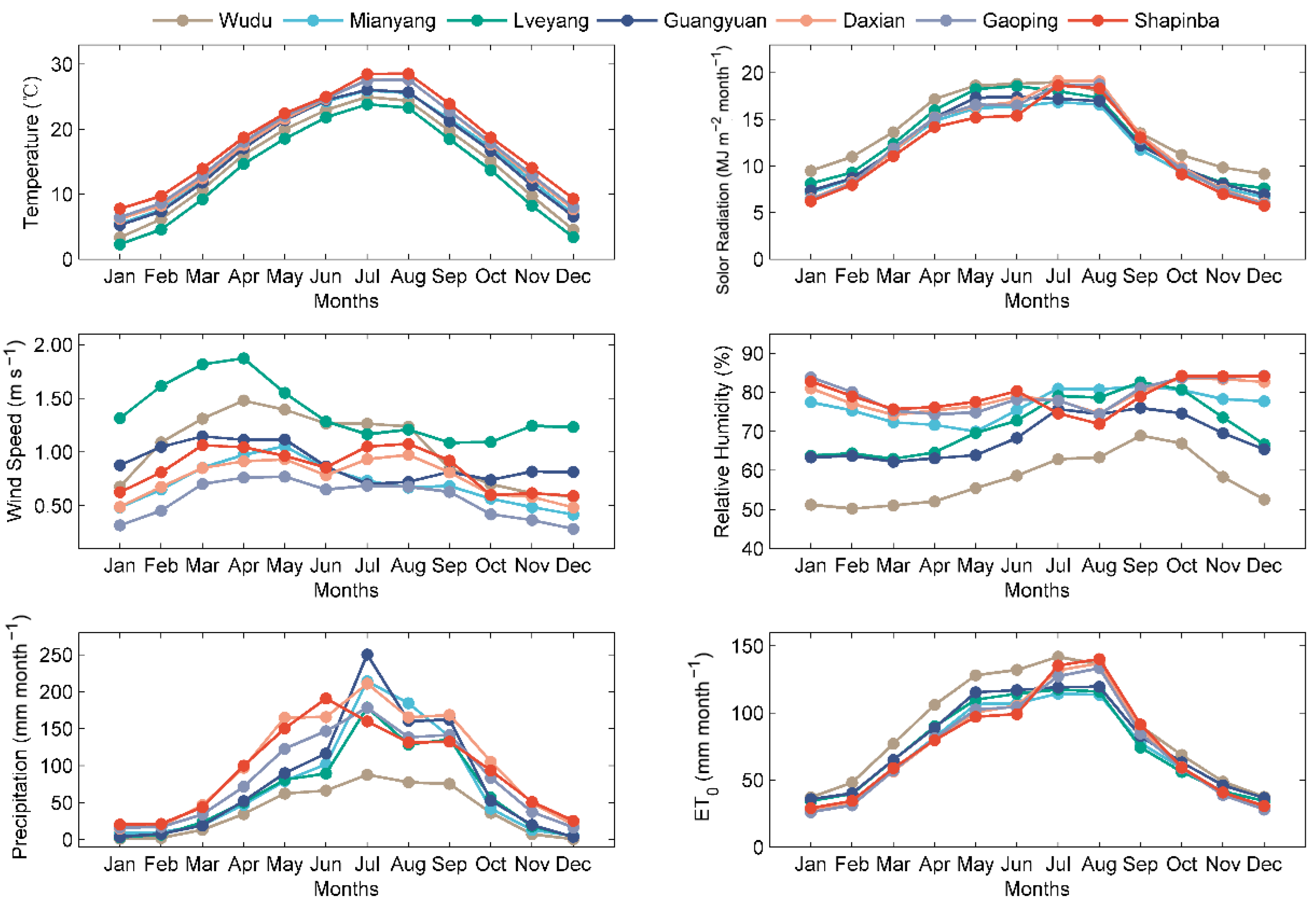
The present study was conducted using seven stations in the JRB: Wudu, Mianyang, Lveyang, Guangyuan, Daxian, Gaoping, and Shapinba. The period from 1964 to 2014 was selected due to the availability of climatic data with few gaps. Monthly climatic data were used in this investigation to estimate monthly ET0. The monthly ET0 values have obvious periodicity [38] and play an important role in planning long-term irrigation management [39]. Therefore, estimating monthly ET0 using machine learning methods is necessary and feasible. The geographical coordinates and the monthly average meteorological parameters are reported in Table 1. Figure 2 shows the monthly variation of the mean air temperature ( T m e a n ), solar radiation ( R s ), wind speed at 2 m height ( u 2 ), relative humidity ( R H ), precipitation, and standard FAO-56 PM ET0 of these meteorological stations. These meteorological datasets were provided by the China Meteorological Data Service Centre (see http://data.cma.cn/en, accessed on 14 April 2021).

2.2. Penman–Monteith Method

The FAO-recommended Penman–Monteith equation (FAO-56 PM) [6] is employed to estimate ET0 data. Given the absence of lysimeter-measured ET0 data, the FAO-56 PM equation is an accepted and widely used practice [40,41]. Thus, the FAO-56 PM equation is considered the benchmark model for the calibration and evaluation of the Hargreaves, Schendel, Irmak, Romanenko, C-ELM, RVM, and ETR models. The equation is given below [6]:
E T 0 = 0.408 Δ ( R n G ) + γ 900 T m e a n + 273 u 2 ( e s e a ) Δ + γ ( 1 + 0.34 u 2 )
where E T 0 is the standardized grass reference evapotranspiration (mm month−1), Δ is the slope of the vapor pressure curve (kPa °C−1), R n is the net radiation at the crop surface (MJ m−2 month−1), G is the soil heat flux (MJ m−2 month−1), T m e a n is the mean air temperature (°C), u 2 is the wind speed at 2 m height (m s−1), e s is the saturation vapor pressure (kPa), e a is the actual vapor pressure (kPa), γ is the air psychometric constant (kPa °C−1).

2.3. Empirical Equations

Four empirical equations were employed to estimate monthly ET0: Hargreaves, Schendel, Irmak, and Romanenko. These equations were locally calibrated using the FAO-56 PM equation to optimize their performance.
The Hargreaves equation [9] is one of the easiest and most accurate equations for estimating ET0. It is described as
E T 0 = a 1 · R s · ( T m e a n + a 2 )
where E T 0 is the reference evapotranspiration (mm month−1), a 1 and a 2 are the empirical coefficients, R s is the solar radiation (MJ m−2 month−1), T m e a n is the monthly mean air temperatures (°C).
The Schendel equation, as described by Schendel [14] is as follows:
E T 0 = a 1 · T m e a n R H
where E T 0 is the reference evapotranspiration (mm month−1), a 1 is the empirical coefficient, T m e a n is the monthly mean air temperature (°C), R H is the relative humidity (%).
Irmak equation [16] is a linear regression equation and can be expressed as
E T 0 = a 1 · R s + a 2 · T m e a n a 3
where E T 0 is the reference evapotranspiration (mm month−1), a 1 , a 2 and a 3 are the empirical coefficients, R s is the solar radiation (MJ m−2 month−1), T m e a n is the monthly mean air temperature (°C).
The Romanenko equation proposed by Romanenko [13] is used to estimate ET0 based on the mean air temperature and relative humidity. It is expressed as
E T 0 = a 1 · ( a 2 + T m e a n ) a 3 · ( a 4 R H )
where E T 0 is the reference evapotranspiration (mm month−1), a 1 , a 2 , a 3 , and a 4 are empirical coefficients, T m e a n is the monthly mean air temperature (°C), R H is the relative humidity (%).

2.4. Relevance Vector Machine

Tipping [30] proposed the relevance vector machine (RVM) as a general-purpose sparse Bayesian modeling method. The RVM model applies automatic relevance determination (ARD) to linear regression to remove parameters that contribute nothing to the construction of the model, resulting in a sparsity model. Therefore, models generated by the RVM are usually more concise than those generated by the corresponding SVM, increasing the speed of processing test data. In the RVM model, most parameters converge to zero during the iterative learning process, while non-zero parameters correspond to points referred to as relevance vectors, which reflect the most essential features of the dataset. The RVM model can utilize non-Mercer kernels and has a fast computation speed compared to the SVM model. Moreover, the RVM model has a high generalization capacity and generates probabilistic interpretation and prediction uncertainties [42]. The kernel function of the RVM model used in this study is sigmoid.

2.5. Complex Extreme Learning Machine

The Complex Extreme Learning Machine (C-ELM) is an ELM-based model developed by Li et al. [31], which has better generalization capability than ELM. The C-ELM model is simple to use and offers a faster learning rate, faster reaction time, and a low symbolic error rate (SER) [43]. When constructing a C-ELM model, the hidden layer bias and input weights (linking the input and hidden layers) are produced at random, and the final output weights (connecting the hidden and output layers) are simply determined mathematically rather than being iteratively tuned. This method eliminates the potential for human error in manually fine-tuning control parameters including starting weights, learning rates, and learning epochs. The analysis of excellent solutions using the C-ELM model can also help prevent local minima. The hyperparameter tested in this study is the hidden layers. The remaining parameters are in the default settings.

2.6. Extremely Randomized Trees

Random Forest (RF) uses a randomized with a put-back approach to obtain the training set of each decision tree, which results in duplicate samples in the training set. The RF model does not guarantee that all samples can be fully utilized, and there may be similarities among decision trees [44]. Based on the above considerations, the extreme random tree (ETR) model was developed by Geurts [32]. Every decision tree in the ETR model is trained utilizing the entire training set, guaranteeing that the training set is fully used and minimizing the final prediction bias. To ensure structural differences among decision trees, the division threshold of each feature is randomly chosen from the sub-datasets, and the feature with the best division is chosen as the satisfactory division attribute by the specified threshold. Therefore, the ETR model is trained faster than the RF. The hyperparameters tested in this study are the number of trees, the number of points for each leaf, and the number of attributes selected to perform the random splits. The rest of the parameters are in the default mode.

2.7. Model Development

In the present study, the RVM, C-ELM, and ETR models were developed and compared with four calibrated empirical equations. ET0 is only affected by climatic data including T m e a n , R s , R H , u 2 , etc. [45]. Temperature and solar radiation data have been proved to be important factors for ET0 estimation [46]. This is consistent with the background theory that temperature and solar radiation are the two main driving forces of ET0 [47]. In the development of ML models, it is desirable to determine the independence of each parameter to reduce complexity and increase efficiency [48]. Utilizing the Pearson’s correlation coefficient is one of the commonly used approaches to check the independence of hydrological parameters. This is a parametric technique, and therefore its application requires the conditions that must be respected in the data set. One of the most crucial assumptions is that the statistical distribution is normal, which is not always true in hydrological data [49]. Additionally, the presence of outlier data may have an impact on the modeling outcomes. As a result, instead of utilizing Pearson’s correlation coefficient to check the independence of the input parameters, this study estimated the accuracy of the ML models with six input combinations of parameters ( T m e a n , R s , R H , and u 2 ) based on the background theory to assess the significance of each climatic parameter and train the ML models.
Table 2 illustrates the six input combinations used in this study. The RVM3, C-ELM3, ETR3, Hargreaves, and Schendel equations have the same input combination ( T m e a n , R s ). The RVM4, C-ELM4, ETR4, Irmak, and Romanenko equations have the same input combination ( T m e a n , R H ).
The entire dataset (data during 1964–2014) was divided into three parts. The first part (data during 1964–2000) was used to train/calibrate the ML models/empirical equations; the second part (data during 2001–2007) was utilized to validate the ML models and empirical equations; the third part (data during 2008–2014) was used to test the calibrated ML models and revised empirical equations. This approach can ensure a high generalization ability and an independent test of the calibrated models [50,51]. Although it is disappointing that the dataset from 2015 to present was not used, similar studies in Iran [49,52] illustrated that 50 years of data are sufficient to meet the objectives of the study.

2.8. Performance Evaluation

This study employed four frequently used statistical metrics to compare empirical equations and ML models to the FAO-56 PM equation: correlation of determination (R2), Nash–Sutcliffe efficiency coefficient (NSE), root mean square error (RMSE), and mean absolute error (MAE). They are defined as
R 2 = ( i = 1 n ( E T 0 , P M , i E T 0 , P M , i ¯ ) ( E T 0 , e , i E T 0 , e , i ¯ ) ) 2 i = 1 n ( E T 0 , P M , i E T 0 , P M , i ¯ ) 2 i = 1 n ( E T 0 , e , i E T 0 , e , i ¯ ) 2
N S E = 1 i = 1 n ( E T 0 , P M , i E T 0 , e , i ) 2 i = 1 n ( E T 0 , P M , i E T 0 , P M , i ¯ ) 2
R M S E = 1 n i = 1 n ( E T 0 , P M , i E T 0 , e , i ) 2
M A E = 1 n i = 1 n | E T 0 , P M , i E T 0 , e , i |
where n is the sample number, E T 0 , P M , i is the standard FAO-56 PM ET0 value, E T 0 , e , i is the model estimated ET0 value, E T 0 , P M , i ¯ is the average FAO-56 PM ET0 value, and E T 0 , e , i ¯ is the average model estimated ET0 value.

3. Results and Discussion

3.1. Estimation of Empirical Models

Table 3 represents the statistical indices of the four empirical equations averaged over the seven stations. In the testing period, the Hargreaves equation is superior to other empirical equations; the R2, NSE, RMSE, and MAE values are calculated as 0.982, 0.957, 7.047 mm month−1, and 5.946 mm month−1, respectively, followed by the Irmak equation (R2 = 0.973, NSE = 0.953, RMSE = 7.588 mm month−1, MAE = 5.983 mm month−1), and the Romanenko equation in third place (R2 = 0.966, NSE = 0.916, RMSE = 9.648 mm month−1, MAE = 7.612 mm month−1). The Schendel equation has the poorest results (R2 = 0.944, NSE = 0.901, RMSE = 11.025 mm month−1, MAE = 8.900 mm month−1).
The R2, NSE, RMSE, and MAE values of the studied empirical equations at different stations are given in Figure 3. In general, the Hargreaves equation performs best at all stations, followed by the Irmak equation. The Romanenko equation is slightly better than the Schendel equation at most stations. The lowest NSE value and highest RMSE value are found at the Daxian station, which has higher precipitation (1228.38 mm) than those of other stations (most < 1000 mm). With the lowest RMSE and MAE values and the highest R2 and NSE values, Lveyang station achieves the best performance.
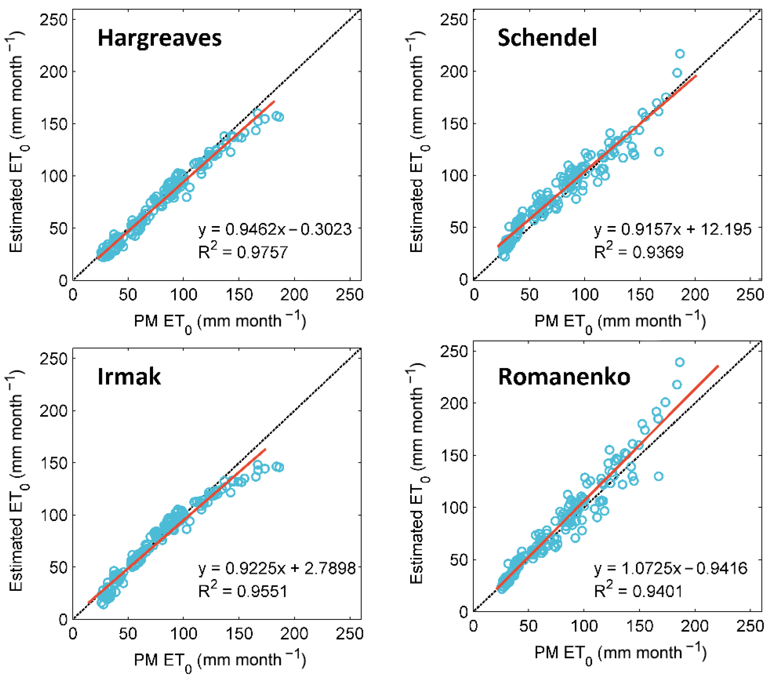
The Shapinba station is a typical station belonging not only to the Jialing River basin but also to the Three Gorges Reservoir area of the Yangtze River. Figure 4 shows the FAO-56 PM ET0 values and empirical equation-estimated ET0 values at Shapinba station during the testing period. The scatter plot of the Hargreaves equation provides accurate results between 0 and 150 mm month−1 but underestimates ET0 when values exceed 150 mm month−1. The Irmak equation performs well from 50 to 150 mm month−1 and underestimates ET0 when values are less than 50 mm month−1 and greater than 150 mm month−1. The Romanenko equation significantly overestimates ET0 and shows more scattered estimates than the others. The Schendel equation overestimates low ET0 values and underestimates high ET0 values. Therefore, the Hargreaves equation is the most accurate of the four empirical models. Our results are consistent with those of Moeletsi et al. [53] and Valipour et al. [54].

3.2. Estimation of Machine Learning Models

Table 4 is created to compare the accuracy of ET0 estimated by the RVM, C-ELM, and ETR models with six input combinations. From Table 4, it is seen that input combination 6 has superior performance to other input combinations. Considering all eighteen ML models, the best model is C-ELM6 (R2 = 0. 995, NSE = 0. 995, RMSE = 2.517 mm month−1, MAE = 1.966 mm month−1), the best model with three input parameters is C-ELM5 (R2 = 0.974, NSE = 0.943, RMSE = 8.293 mm month−1, MAE = 6.570 mm month−1), the best model with two input parameters is C-ELM3 (R2 = 0.985, NSE = 0.966, RMSE = 6.153 mm month−1, NSE = 4.988 mm month−1), and the best model with only one input parameter is RVM2 (R2 = 0.946, NSE = 0.909, RMSE = 10.626 mm month−1, MAE = 8.652 mm month−1).
Figure 5 shows the RMSE values of the RVM, C-ELM, and ETR models with six input combinations. According to Figure 5, when input parameters are combinations 1–4, the RVM, C-ELM, and ETR models present similar estimation accuracy. When input parameters are combinations 5–6, the C-ELM model gives better performance than the RVM and ETR models. Otherwise, combination 2 gives lower RMSE values than those of combination 1. The combination 3 also gives quite good results. The RMSE of combination 5 has little significant improvement compared to combination 4. The results show that R s has the greatest effect on estimating monthly ET0 in this humid study area, followed by T m e a n and R H . The minimum effective input parameter is determined as u 2 for the RVM, CELM, and ETR models.
From Table 4 and Figure 5, the C-ELM model is superior to the RVM and ETR models. Figure 6 is intended to investigate the accuracy of the C-ELM model with six input combinations. As can be seen from Figure 6, the scatter plot of C-ELM6 is less scattered. Among the models investigated, the C-ELM6 model has the best fit line and the highest R2 value (R2 = 0.9949). The C-ELM4 and C-ELM5 models invariably overestimate the ET0 values. The R2 values of the C-ELM4 and C-ELM5 are 0.9836 and 0.9842, respectively. The fitting slopes of C-ELM1, C-ELM2, and C-ELM3 are between 0.83 and 0.99, indicating those models underestimate the ET0 values. The C-ELM1 and C-ELM2 models with one input parameter are more scattered than the other models. The C-ELM3 model with two input parameters is less distributed and produces reliable results (R2 = 0.9855). Overall, C-ELM3 and C-ELM6 are recommended to estimate monthly ET0 values.

3.3. Comparison of Empirical and Machine Learning Models

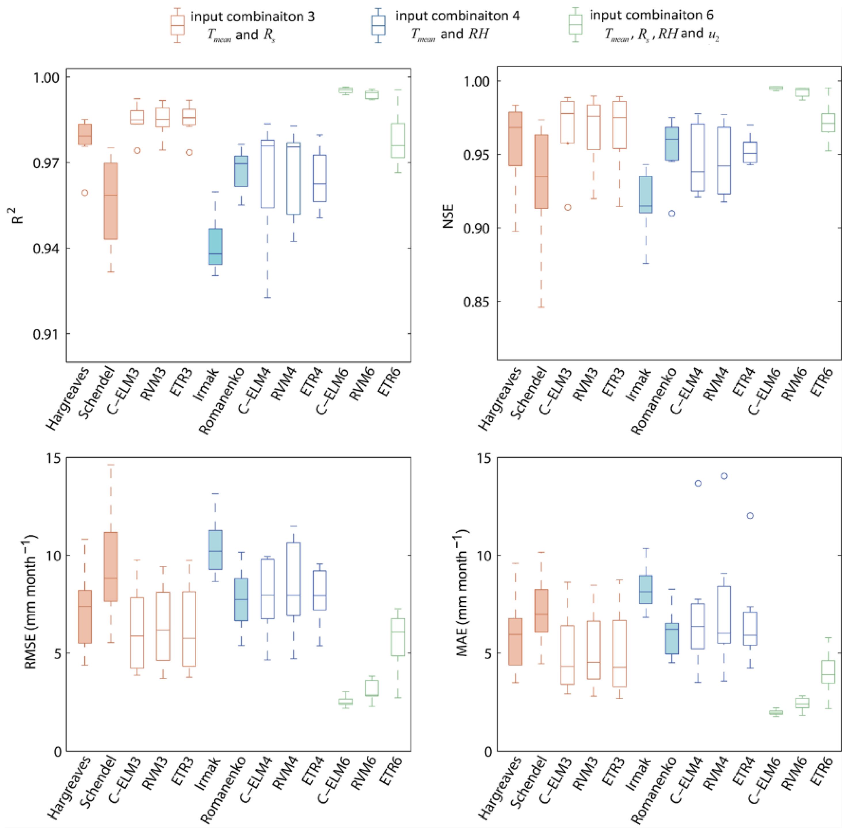
Figure 7 presents the boxplots of statistical indices for the four empirical equations and studied ML models with input combinations 3, 4, and 6. As shown in Figure 7, the C-ELM6, RVM6, and ETR6 models offer the best outcomes compared to other empirical equations and ML models. The C-ELM6 model has the highest values for R2 and NSE and the lowest values for RMSE and MAE, followed by the RVM6 model, with the ETR6 model in third place. When T m e a n and R s are the inputs, The C-ELM3, RVM3, and ETR3 models give better performance than the Hargreaves and Schendel equations. When T m e a n and R H are the inputs, the C-ELM3, RVM3, ETR3, and Romanenko equations have similar accuracy, but the Irmak equation has the worst performance. In conclusion, the ML models exhibit superior performance compared to the four empirical equations, and the C-ELM6 model is the best model.
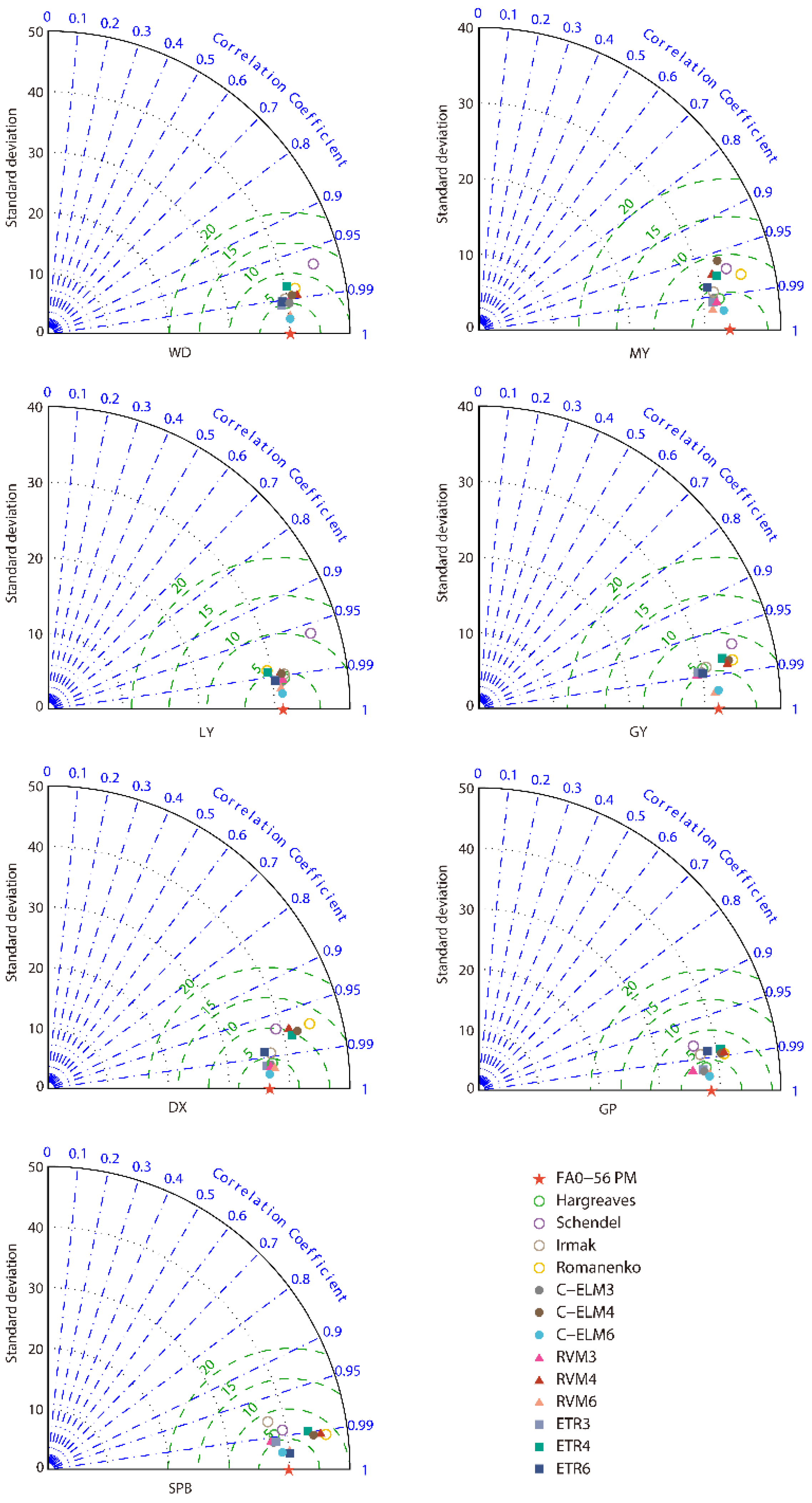
The Taylor diagram is created to study the adaptation between FAO-56 PM ET0 and estimated ET0 (Figure 8). As displayed in Figure 8, the C-ELM6, RVM6, and ETR6 models perform quite well. The most accurate model compared to FAO-56 PM ET0 for the seven stations except Shapinba is the C-ELM6 model. At the Shapinba station, the best model is the ETR6 model. Overall, the C-ELM6 model and Schendel equation yield the highest and lowest accordance, respectively, with the FAO-56 PM standard deviation line.

4. Conclusions

In this study, for the first time, four empirical equations (Hargreaves, Schendel, Irmak, and Romanenko) and three ML models (RVM, C-ELM, and ETR) were established for estimating monthly ET0 in the JRB. Monthly meteorological datasets including T m e a n , R s , R H , and u 2 from the seven meteorological stations in this Basin for 1964–2014 were used. Based on the obtained results, some conclusions can be drawn.
Firstly, R s and T m e a n were considered to have significant effects on ET0, especially under humid conditions. R H and u 2 produced less meaningful results when used separately. Nevertheless, adding R H and u 2 to R s or T m e a n improved the accuracy for estimating monthly ET0.
Secondly, four empirical equations (Hargreaves, Schendel, Irmak, and Romanenko) had acceptable estimation accuracy. The Hargreaves equation was the best empirical equation in the JRB. However, all ML models had more accurate results compared to empirical equations. Therefore, it can be confirmed that the RVM, C-ELM, and ETR models are efficient methods to get satisfactory results for estimating monthly ET0. The RVM and ETR models showed similar ability. The C-ELM performed better than the RVM and ETR models. Moreover, the C-ELM6 model, which uses T m e a n , R s , R H , and u 2 as inputs, produced the best estimates.
Finally, this study conclusively substantiated the effectiveness and generalization performance of ML techniques (RVM, C-ELM, and ETR) for modeling and forecasting ET0, which was also the first attempt to investigate the JRB with a subtropical humid monsoon climate. Nevertheless, under other climatic conditions, the applicability and validity of these advanced regression techniques remain to be investigated. More importantly, with the development of remote sensing techniques, using satellite remote sensing datasets combined with meteorological datasets needs to be studied to further improve the accuracy of ML models.

Author Contributions

X.D. and J.L. conceived the experiment and curated the data; J.L. performed the analysis and drafted the manuscript; X.D. and M.M. reviewed and edited the manuscript; X.D. and M.M. acquired funding. All authors have read and agreed to the published version of the manuscript.

Funding

This research was jointly supported by the National Natural Science Foundation of China projects (grant number: 41830648), the National Major Projects on High-Resolution Earth Observation System (No. 21-Y20B01-9001-19/22), and the Fundamental Research Funds for the Central Universities (No. SWU118062).

Institutional Review Board Statement

Not applicable.

Informed Consent Statement

Not applicable.

Data Availability Statement

All data required to evaluate the conclusions in the research are present in the paper. Additional data related to this research may be requested from the authors.

Acknowledgments

We would like to express our appreciation to the Chinese Meteorological Administration Bureau for supplying the meteorological data for this work.

Conflicts of Interest

The authors declare no conflict of interest.

References

  1. Gutierrez, S.C.; Cajachagua, H.S.; Huanca, M.S.; Rojas, J.F.; Vidal, Y.S.; Cuxart, J. Seasonal variability of daily evapotranspiration and energy fluxes in the Central Andes of Peru using eddy covariance techniques and empirical methods. Atmos. Res. 2021, 261, 105760. [Google Scholar] [CrossRef]
  2. Smith, M. The application of climatic data for planning and management of sustainable rainfed and irrigated crop production. Agric. For. Meteorol. 2000, 103, 99–108. [Google Scholar] [CrossRef]
  3. Fan, J.; Ma, X.; Wu, L.; Zhang, F.; Yu, X.; Zeng, W. Light Gradient Boosting Machine: An efficient soft computing model for estimating daily reference evapotranspiration with local and external meteorological data. Agric. Water Manag. 2019, 225, 105758. [Google Scholar] [CrossRef]
  4. Rafi, Z.; Merlin, O.; Le Dantec, V.; Khabba, S.; Mordelet, P.; Er-Raki, S.; Amazirh, A.; Olivera-Guerra, L.; Ait Hssaine, B.; Simonneaux, V.; et al. Partitioning evapotranspiration of a drip-irrigated wheat crop: Inter-comparing eddy covariance-, sap flow-, lysimeter- and FAO-based methods. Agric. For. Meteorol. 2019, 265, 310–326. [Google Scholar] [CrossRef]
  5. Anapalli, S.S.; Fisher, D.K.; Reddy, K.N.; Wagle, P.; Gowda, P.H.; Sui, R. Quantifying soybean evapotranspiration using an eddy covariance approach. Agric. Water Manag. 2018, 209, 228–239. [Google Scholar] [CrossRef]
  6. Allen, R.G.; Pereira, L.S.; Raes, D.; Smith, M. Crop evapotranspiration-Guidelines for computing crop water requirements-FAO Irrigation and drainage paper 56. Fao Rome 1998, 300, D05109. [Google Scholar]
  7. Valiantzas, J.D. Simplified forms for the standardized FAO-56 Penman–Monteith reference evapotranspiration using limited weather data. J. Hydrol. 2013, 505, 13–23. [Google Scholar] [CrossRef]
  8. Hargreaves, G.H.; Samani, Z.A. Reference crop evapotranspiration from temperature. Appl. Eng. Agric. 1985, 1, 96–99. [Google Scholar] [CrossRef]
  9. Hargreaves, G.H. Moisture Availability and Crop Production. Trans. ASAE 1975, 18, 980–0984. [Google Scholar] [CrossRef]
  10. Turc, L. Estimation of irrigation water requirements, potential evapotranspiration: A simple climatic formula evolved up to date. Ann. Agron. 1961, 12, 13–49. [Google Scholar]
  11. Tabari, H. Evaluation of Reference Crop Evapotranspiration Equations in Various Climates. Water Resour. Manag. 2010, 24, 2311–2337. [Google Scholar] [CrossRef]
  12. Trabert, W. Neue beobachtungen über verdampfungsgeschwindigkeiten. Meteorol. Z 1896, 13, 261–263. [Google Scholar]
  13. Romanenko, V. Computation of the autumn soil moisture using a universal relationship for a large area. Proc. Ukr. Hydrometeorol. Res. Ins. 1961, 3, 12–25. [Google Scholar]
  14. Schendel, U. Vegetationswasserverbrauch und-wasserbedarf. Habilit. Kiel 1967, 137, 1–11. [Google Scholar]
  15. Djaman, K.; Balde, A.B.; Sow, A.; Muller, B.; Irmak, S.; N’Diaye, M.K.; Manneh, B.; Moukoumbi, Y.D.; Futakuchi, K.; Saito, K. Evaluation of sixteen reference evapotranspiration methods under sahelian conditions in the Senegal River Valley. J. Hydrol. Reg. Stud. 2015, 3, 139–159. [Google Scholar] [CrossRef]
  16. Irmak, S.; Irmak, A.; Allen, R.; Jones, J. Solar and net radiation-based equations to estimate reference evapotranspiration in humid climates. J. Irrig. Drain. Eng. 2003, 129, 336–347. [Google Scholar] [CrossRef]
  17. Priestley, C.H.B.; Taylor, R.J. On the assessment of surface heat flux and evaporation using large-scale parameters. Mon. Weather Rev. 1972, 100, 81–92. [Google Scholar] [CrossRef]
  18. Tabari, H.; Grismer, M.E.; Trajkovic, S. Comparative analysis of 31 reference evapotranspiration methods under humid conditions. Irrig. Sci. 2013, 31, 107–117. [Google Scholar] [CrossRef]
  19. Djaman, K.; Koudahe, K.; Sall, M.; Kabenge, I.; Rudnick, D.; Irmak, S. Performance of Twelve Mass Transfer Based Reference Evapotranspiration Models under Humid Climate. J. Water Resour. Prot. 2017, 09, 1347–1363. [Google Scholar] [CrossRef] [Green Version]
  20. Gong, X.; Qiu, R.; Ge, J.; Bo, G.; Ping, Y.; Xin, Q.; Wang, S. Evapotranspiration partitioning of greenhouse grown tomato using a modified Priestley–Taylor model. Agric. Water Manag. 2021, 247, 106709. [Google Scholar] [CrossRef]
  21. Valle Júnior, L.C.G.; Ventura, T.M.; Gomes, R.S.R.; de S. Nogueira, J.; de A. Lobo, F.; Vourlitis, G.L.; Rodrigues, T.R. Comparative assessment of modelled and empirical reference evapotranspiration methods for a brazilian savanna. Agric. Water Manag. 2020, 232, 106040. [Google Scholar] [CrossRef]
  22. Wen, X.; Si, J.; He, Z.; Wu, J.; Shao, H.; Yu, H. Support-Vector-Machine-Based Models for Modeling Daily Reference Evapotranspiration With Limited Climatic Data in Extreme Arid Regions. Water Resour. Manag. 2015, 29, 3195–3209. [Google Scholar] [CrossRef]
  23. Citakoglu, H.; Cobaner, M.; Haktanir, T.; Kisi, O. Estimation of Monthly Mean Reference Evapotranspiration in Turkey. Water Resour. Manag. 2013, 28, 99–113. [Google Scholar] [CrossRef]
  24. Cobaner, M. Evapotranspiration estimation by two different neuro-fuzzy inference systems. J. Hydrol. 2011, 398, 292–302. [Google Scholar] [CrossRef]
  25. Feng, Y.; Cui, N.; Zhao, L.; Hu, X.; Gong, D. Comparison of ELM, GANN, WNN and empirical models for estimating reference evapotranspiration in humid region of Southwest China. J. Hydrol. 2016, 536, 376–383. [Google Scholar] [CrossRef]
  26. Falamarzi, Y.; Palizdan, N.; Huang, Y.F.; Lee, T.S. Corrigendum to “Estimating evapotranspiration from temperature and wind speed data using artificial and wavelet neural networks (WNNs)” [Agric. Water Manag. 140 (2014) 26–36]. Agric. Water Manag. 2016, 164, 340. [Google Scholar] [CrossRef]
  27. Xu, C.Y.; Singh, V. Evaluation and generalization of radiation-based methods for calculating evaporation. Hydrol. Process. 2000, 14, 339–349. [Google Scholar] [CrossRef]
  28. Fan, J.; Yue, W.; Wu, L.; Zhang, F.; Cai, H.; Wang, X.; Lu, X.; Xiang, Y. Evaluation of SVM, ELM and four tree-based ensemble models for predicting daily reference evapotranspiration using limited meteorological data in different climates of China. Agric. For. Meteorol. 2018, 263, 225–241. [Google Scholar] [CrossRef]
  29. Bellido-Jiménez, J.A.; Estévez, J.; García-Marín, A.P. New machine learning approaches to improve reference evapotranspiration estimates using intra-daily temperature-based variables in a semi-arid region of Spain. Agric. Water Manag. 2021, 245, 106558. [Google Scholar] [CrossRef]
  30. Tipping, M.E. Sparse Bayesian learning and the relevance vector machine. J. Mach. Learn. Res. 2001, 1, 211–244. [Google Scholar]
  31. Li, M.-B.; Huang, G.-B.; Saratchandran, P.; Sundararajan, N. Fully complex extreme learning machine. Neurocomputing 2005, 68, 306–314. [Google Scholar] [CrossRef]
  32. Geurts, P.; Ernst, D.; Wehenkel, L. Extremely randomized trees. Mach. Learn. 2006, 63, 3–42. [Google Scholar] [CrossRef] [Green Version]
  33. Deo, R.C.; Samui, P.; Kim, D. Estimation of monthly evaporative loss using relevance vector machine, extreme learning machine and multivariate adaptive regression spline models. Stoch. Environ. Res. Risk Assess. 2015, 30, 1769–1784. [Google Scholar] [CrossRef]
  34. Tripathi, S.; Govindaraju, R.S. On selection of kernel parametes in relevance vector machines for hydrologic applications. Stoch. Environ. Res. Risk Assess. 2006, 21, 747–764. [Google Scholar] [CrossRef]
  35. Saeed, U.; Jan, S.U.; Lee, Y.-D.; Koo, I. Fault diagnosis based on extremely randomized trees in wireless sensor networks. Reliab. Eng. Syst. Saf. 2021, 205, 107284. [Google Scholar] [CrossRef]
  36. Herath, I.K.; Ye, X.; Wang, J.; Bouraima, A.-K. Spatial and temporal variability of reference evapotranspiration and influenced meteorological factors in the Jialing River Basin, China. Theor. Appl. Climatol. 2017, 131, 1417–1428. [Google Scholar] [CrossRef]
  37. Zhang, J.; Zhang, M.; Song, Y.; Lai, Y. Hydrological simulation of the Jialing River Basin using the MIKE SHE model in changing climate. J. Water Clim. Chang. 2021, 12, 2495–2514. [Google Scholar] [CrossRef]
  38. Luo, Y.; Chang, X.; Peng, S.; Khan, S.; Wang, W.; Zheng, Q.; Cai, X. Short-term forecasting of daily reference evapotranspiration using the Hargreaves–Samani model and temperature forecasts. Agric. Water Manag. 2014, 136, 42–51. [Google Scholar] [CrossRef]
  39. Luo, Y.; Traore, S.; Lyu, X.; Wang, W.; Wang, Y.; Xie, Y.; Jiao, X.; Fipps, G. Medium range daily reference evapotranspiration forecasting by using ANN and public weather forecasts. Water Resour. Manag. 2015, 29, 3863–3876. [Google Scholar] [CrossRef]
  40. Zhou, Z.; Zhao, L.; Lin, A.; Qin, W.; Lu, Y.; Li, J.; Zhong, Y.; He, L. Exploring the potential of deep factorization machine and various gradient boosting models in modeling daily reference evapotranspiration in China. Arab. J. Geosci. 2021, 13, 1–20. [Google Scholar] [CrossRef]
  41. Zhang, Y.; Zhao, Z.; Zheng, J. CatBoost: A new approach for estimating daily reference crop evapotranspiration in arid and semi-arid regions of Northern China. J. Hydrol. 2020, 588, 125087. [Google Scholar] [CrossRef]
  42. Samui, P.; Dixon, B. Application of support vector machine and relevance vector machine to determine evaporative losses in reservoirs. Hydrol. Processes 2012, 26, 1361–1369. [Google Scholar] [CrossRef]
  43. Nazhad, S.H.H.; Lotfinejad, M.M.; Danesh, M.; Amin, R.U.; Shamshirband, S. A comparison of the performance of some extreme learning machine empirical models for predicting daily horizontal diffuse solar radiation in a region of southern Iran. Int. J. Remote Sens. 2017, 38, 6894–6909. [Google Scholar] [CrossRef]
  44. Breiman, L. Random forests. Mach. learn. 2001, 45, 5–32. [Google Scholar] [CrossRef] [Green Version]
  45. Adamala, S.; Raghuwanshi, N.; Mishra, A.; Singh, R. Generalized wavelet neural networks for evapotranspiration modeling in India. ISH J. Hydraul. Eng. 2019, 25, 119–131. [Google Scholar] [CrossRef]
  46. Dong, J.; Liu, X.; Huang, G.; Fan, J.; Wu, L.; Wu, J. Comparison of four bio-inspired algorithms to optimize KNEA for predicting monthly reference evapotranspiration in different climate zones of China. Comput. Electron. Agric. 2021, 186, 106211. [Google Scholar] [CrossRef]
  47. Chia, M.Y.; Huang, Y.F.; Koo, C.H.; Fung, K.F. Recent advances in evapotranspiration estimation using artificial intelligence approaches with a focus on hybridization techniques—A review. Agronomy 2020, 10, 101. [Google Scholar] [CrossRef] [Green Version]
  48. Lin, H.-M.; Chang, S.-K.; Wu, J.-H.; Juang, C.H. Neural network-based model for assessing failure potential of highway slopes in the Alishan, Taiwan Area: Pre-and post-earthquake investigation. Eng. Geol. 2009, 104, 280–289. [Google Scholar] [CrossRef]
  49. Ahmadi, F.; Mehdizadeh, S.; Mohammadi, B.; Pham, Q.B.; Doan, T.N.C.; Vo, N.D. Application of an artificial intelligence technique enhanced with intelligent water drops for monthly reference evapotranspiration estimation. Agric. Water Manag. 2021, 244, 106622. [Google Scholar] [CrossRef]
  50. Dou, X.; Yang, Y. Estimating forest carbon fluxes using four different data-driven techniques based on long-term eddy covariance measurements: Model comparison and evaluation. Sci Total Environ. 2018, 627, 78–94. [Google Scholar] [CrossRef] [PubMed]
  51. Karimi, S.; Shiri, J.; Marti, P. Supplanting missing climatic inputs in classical and random forest models for estimating reference evapotranspiration in humid coastal areas of Iran. Comput. Electron. Agric. 2020, 176, 105633. [Google Scholar] [CrossRef]
  52. Gavili, S.; Sanikhani, H.; Kisi, O.; Mahmoudi, M.H. Evaluation of several soft computing methods in monthly evapotranspiration modelling. Meteorol. Appl. 2018, 25, 128–138. [Google Scholar] [CrossRef] [Green Version]
  53. Moeletsi, M.E.; Walker, S.; Hamandawana, H. Comparison of the Hargreaves and Samani equation and the Thornthwaite equation for estimating dekadal evapotranspiration in the Free State Province, South Africa. Phys. Chem. Earth 2013, 66, 4–15. [Google Scholar] [CrossRef]
  54. Valipour, M.; Sefidkouhi, M.A.G.; Raeini-Sarjaz, M. Spatiotemporal Analysis of Reference Evapotranspiration in Arid, Semiarid, Mediterranean and Very Humid Climates Considering Developed Models and Lysimeter Measurements. Water Conserv. Sci. Eng. 2020, 5, 81–96. [Google Scholar] [CrossRef]
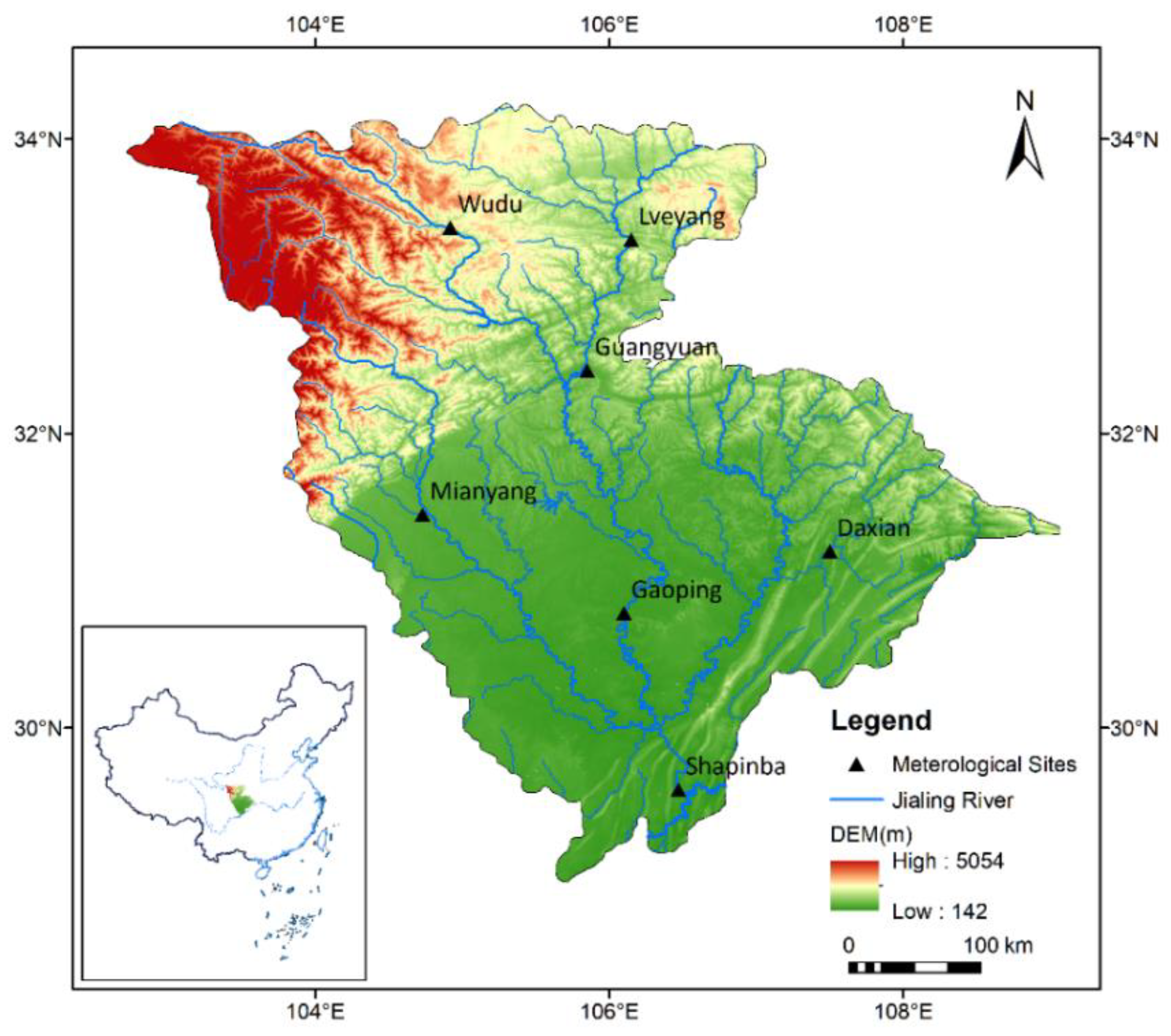
Figure 1. The geographical location of the study area.
Ijerph 19 13127 g001
Figure 2. Monthly variations of meteorological parameters and ET0 for seven studied meteorological stations during 1964–2014.
Ijerph 19 13127 g002
Figure 3. Statistical indices of the four calibrated empirical equations at the seven stations for modeling ET0 during the testing period (2008–2014). WD-Wudu, MY-Mianyang, LY-Lveyang, GY-Guangyuan, DX-Daxian, GP-Gaoping, SPB-Shapinba.
Ijerph 19 13127 g003
Figure 4. Scatter plots of ET0 values estimated by the four empirical models against FAO-56 PM ET0 values at Shapinba station during the testing period.
Ijerph 19 13127 g004
Figure 5. RMSE values of the RVM, C-ELM, and ETR models with six input combinations at the seven stations for modeling ET0 during the testing period (2008–2014). WD-Wudu, MY-Mianyang, LY-Lveyang, GY-Guangyuan, DX-Daxian, GP-Gaoping, SPB-Shapinba.
Ijerph 19 13127 g005
Figure 6. Scatter plots of ET0 values estimated by the C-ELM model against FAO-56 PM ET0 values at Shapinba station during the testing period.
Ijerph 19 13127 g006
Figure 7. Boxplot of statistical indices for the four empirical equations and ML models for predicting ET0 with input combinations 3, 4, and 6. Solid boxes are empirical equations, and blank boxes are ML models.
Ijerph 19 13127 g007
Figure 8. Taylor diagrams for the four empirical equations and RVM, C-ELM, and ETR models for predicting ET0 at the seven stations.
Ijerph 19 13127 g008
Table 1. Meteorological stations with monthly average climatic conditions (from 1964 to 2014). T m e a n is the monthly mean air temperature (°C), R s is the monthly solar radiation (MJ m−2 month-1), u 2 is the monthly wind speed at 2 m height (m s−1), R H is the monthly relative humidity (%), ET0 is the monthly standard FAO-56 PM ET0 values (mm month-1), and precipitation is the average annual rainfall (mm).
SitesLatitude
(° N)
Longitude
(° E)
Altitude
(m)
T m e a n
R s
u 2
R H
ET0Precipitation
Wudu33.40104.921079.114.8214.121.5457.6587.66466.29
Mianyang31.45104.73522.716.4511.961.2076.8770.95865.49
Lveyang33.32106.15794.213.5012.991.8771.6474.42776.57
Guangyuan32.43105.85513.816.2612.401.4068.3877.47939.32
Daxian31.20107.50344.317.2412.471.2578.8073.991228.38
Gaoping30.78106.10309.717.4812.321.0679.3472.791005.38
Shapinba29.58106.47259.118.4011.831.3579.1674.711121.27
Table 2. Summary of the six input combinations of the meteorological parameters used in the RVM, C-ELM, and ETR models.
CombinationRVMC-ELMETRInput Combination
1RVM1C-ELM1ETR1 T m e a n
2RVM2C-ELM2ETR2 R s
3RVM3C-ELM3ETR3 T m e a n ,   R s
4RVM4C-ELM4ETR4 T m e a n ,   R H
5RVM5C-ELM5ETR5 T m e a n ,   R H ,   u 2
6RVM6C-ELM6ETR6 T m e a n ,   R s ,   R H ,   u 2
Table 3. Statistical indices of the studied empirical equations for modeling ET0 at the seven stations.
Model HargreavesSchendelIrmakRomanenko
CalibrationR20.980.9420.9730.964
NSE0.9790.9290.9730.964
RMSE5.2019.6896.0276.959
MAE3.9837.7664.5815.381
ValidationR20.9760.9460.9650.956
NSE0.9580.9320.9540.941
RMSE7.0799.6217.778.751
MAE5.7637.6796.0126.587
TestingR20.9820.9440.9730.966
NSE0.9570.9010.9530.916
RMSE7.04711.0257.5889.648
MAE5.9468.95.9837.612
Table 4. Statistical indices for the RVM, C-ELM, and ETR models with six input combinations for modeling ET0 during the training, validation, and testing periods.
ModelRVM1RVM2RVM3RVM4RVM5RVM6C-ELM1C-ELM2C-ELM3C-ELM4C-ELM5C-ELM6ETR1ETR2ETR3ETR4ETR5ETR6
TrainingR20.912 0.943 0.986 0.972 0.976 0.993 0.9130.9440.986 0.9720.9780.9940.922 0.948 0.988 0.976 0.981 0.993
NSE0.912 0.943 0.985 0.972 0.948 0.993 0.9130.9440.986 0.9720.9780.994 0.922 0.948 0.988 0.976 0.981 0.993
RMSE10.7408.748 4.313 6.153 7.409 2.977 10.682 8.6934.195 6.0995.3622.70910.1138.423 3.948 5.661 5.063 2.955
MAE8.460 6.927 3.190 4.550 5.797 2.120 8.418 6.8693.076 4.4993.8671.9087.941 6.662 2.834 4.244 3.736 2.063
ValidationR20.890 0.935 0.979 0.957 0.952 0.992 0.886 0.9350.981 0.9590.968 0.9940.883 0.934 0.981 0.957 0.950 0.972
NSE0.886 0.908 0.967 0.950 0.908 0.991 0.882 0.9060.969 0.9490.9510.9930.879 0.907 0.968 0.953 0.941 0.967
RMSE12.41411.0206.318 8.100 9.956 3.406 12.665 11.081 5.975 8.1777.9062.97812.82611.0956.189 7.935 8.610 5.996
MAE9.890 8.845 4.912 6.066 7.819 2.571 10.032 8.8934.719 6.0826.026 2.26810.0738.830 4.838 6.012 6.520 4.314
TestingR20.890 0.946 0.985 0.967 0.969 0.994 0.8900.9450.9850.9650.974 0.9950.890 0.944 0.985 0.965 0.962 0.978
NSE0.866 0.909 0.965 0.926 0.881 0.992 0.8650.9070.9660.9270.943 0.9950.866 0.907 0.965 0.937 0.944 0.972
RMSE12.81510.6266.287 9.148 11.0163.069 12.860 10.720 6.153 9.0348.293 2.51712.80010.7736.246 8.688 8.446 5.716
MAE10.0018.652 5.106 7.208 9.077 2.396 10.049 8.7424.9886.9936.5701.9669.966 8.715 5.040 6.668 6.465 4.000
Publisher’s Note: MDPI stays neutral with regard to jurisdictional claims in published maps and institutional affiliations.