Article

State Trends of Cannabis Liberalization as a Causal Driver of Increasing Testicular Cancer Rates across the USA

by
Albert Stuart Reece
1,2,* and
Gary Kenneth Hulse
1,2
1
Division of Psychiatry, University of Western Australia, Crawley, WA 6009, Australia
2
School of Medical and Health Sciences, Edith Cowan University, Joondalup, WA 6027, Australia
*
Author to whom correspondence should be addressed.
Int. J. Environ. Res. Public Health 2022, 19(19), 12759; https://doi.org/10.3390/ijerph191912759
Submission received: 3 August 2022 / Revised: 18 September 2022 / Accepted: 30 September 2022 / Published: 5 October 2022

Abstract

:
Background. The cause of the worldwide doubling-tripling of testicular cancer rates (TCRs) in recent decades is unknown. Previous cohort studies associated cannabis use with TCR including dose–response relationships but the contribution of cannabis to TCRs at the population level is unknown. This relationship was tested by analyzing annual trends across US states and formally assessed causality. Four US datasets were linked at state level: age-adjusted TCRs from Centers for Disease Control Surveillance Epidemiology and End Results database; drug use data from annual National Survey of Drug Use and Health including 74.1% response rate; ethnicity and median household income data from the US Census Bureau; and cannabinoid concentration data from Drug Enforcement Agency reports. Data was processed in R in spatiotemporal and causal inference protocols. Results. Cannabis-use quintile scatterplot-time and boxplots closely paralleled those for TCRs. The highest cannabis-use quintile had a higher TCR than others (3.44 ± 0.05 vs. 2.91 ± 0.2, mean ± S.E.M., t = 10.68, p = 1.29 × 10⁻²²). A dose–response relationship was seen between TCR and Δ9-tetrahydrocannabinol (THC), cannabinol, cannabigerol, and cannabichromene (6.75 × 10⁻⁹ < p < 1.83 × 10−142). In a multivariate inverse probability-weighted interactive regression including race and ethnic cannabis exposure (ECE), ECE was significantly related to TCR (β-estimate = 0.89 (95%C.I. 0.36, 2.67), p < 2.2 × 10⁻¹⁶). In an additive geospatiotemporal model controlling for other drugs, cannabis alone was significant (β-estimate = 0.19 (0.10, 0.28), p = 3.4 × 10⁻⁵). In a full geospatial model including drugs, income and ethnicity cannabinoid exposure was significant (cannabigerol: β-estimate = 1.39 (0.024, 2.53), p = 0.0017); a pattern repeated at two spatial and two temporal lags (cannabigerol: β-estimate = 0.71 (0.05, 1.37), p = 0.0.0350; THC: β-estimate = 23.60 (11.92, 35.29), p = 7.5 × 10⁻⁵). 40/41 e-Values > 1.25 ranged up to 1.4 × 1063 and 10 > 1000 fitting causal relationship criteria. Cannabis liberalization was associated with higher TCRs (ChiSqu. = 312.2, p = 2.64 × 10⁻¹¹). Rates of TC in cannabis-legal states were elevated (3.36 ± 0.09 vs. 3.01 ± 0.03, t = 4.69, p = 4.86 × 10⁻⁵). Conclusions. Cannabis use is closely and causally associated with TCRs across both time and space and higher in States with liberal cannabis legislation. Strong dose–response effects were demonstrated for THC, cannabigerol, cannabinol, cannabichromene and cannabidiol. Cannabinoid genotoxicity replicates all major steps to testicular carcinogenesis including whole-genome doubling, chromosomal arm excision, generalized DNA demethylation and chromosomal translocations thereby accelerating the pathway to testicular carcinogenesis by several decades.

1. Background

1.1. Incidence

Testicular cancer (TC) is the most common cancer in males aged 15–44 years, and responsible for more years of life lost than any other adult cancer [1]. In recent decades, testicular cancer rates (TCRs) have unexplainably risen two- to three- fold in many nations [2,3,4].
Testicular germ cell tumours (TGCT) comes in many variants. In males aged 15–44 years it is usually of either of the seminoma (50%) or non-seminoma (40%) variety, with 10% being of mixed subtype [1,4,5,6,7]. Non-seminoma germ cell tumours (NSGCT) can be of either the embryonal or teratoma or yolk sac or choriocarcinoma varieties depending on whether embryonal tissues or extraembryonal tissues are developed [8]. Germ cell neoplasia in situ (GCNIS) is believed to be the tissue of origin of seminoma; GCNIS or seminoma is believed to be the tissue of origin of embryonal carcinoma which is believed to be the source of extraembryonic (yolk sac or choriocarcinoma) and somatic (teratoma) lineages [8].
Twenty-fold variation in TCR have been documented around the world [1,2,3,4,8] with two-fold variations across the same continent [3], and even within the same country as geographic clusters [9].
SEER*Explorer is an online data portal maintained by the Centers for Disease Control and the National Cancer Institute. It allows online checking of many features of cancer epidemiology such as short and long term trends, age-, sex- and ethnic- specific rates in both tabular and graphical formats. Data from SEER*Explorer reveals that the age-adjusted rate of testicular cancer in US males for all ages and all stages rose 83.45% from 3.4415 to 6.3136/100,000 1976–2017 [10]. When considering the change in the peak age incidence of males 15–39 years the rate rose 92.14% from 6.2922 to 12.091/100,000 1975 to 2017 which represented an annual percent change of 3.31% 1975–1986 and 0.7424 1987–2017. The cause of these concerning rises in TCR is unknown.

1.2. Risk Factors

Many risk factors have been described for TGCT including cryptorchidism, testicular dysgenesis syndrome including congenital urogenital anomalies including hypospadias, infertility, inguinal hernia repair, having a previous TGCT, having a close family relative with TGCT (eight to ten-fold for a brother and four to six- fold for a father), exposure to three organochlorines (dichlorodiphenyldichloroethylene, cis-nonachlor and trans-nonachlor) and certain occupational groups such as firemen and aircraft workers [1,4,6]. Endocrine disruption such as maternal bleeding, low birthweight, twinship, short gestation, tall stature, first position in the sibship and small sibship, Downs syndrome and Klinefelters syndrome are also implicated [4,5], as is the use of cannabis both through gestational exposure and adult use [4,11].
All four studies to have examined the association between TC and cannabis use have found a positive relationship [12,13,14,15]. Dose response relationships have been demonstrated for frequency of use [13,15], for long term use [15], for total dose exposure (more than 50 times) [12] and the age of first onset (less than or older than eighteen years of age) [13]. Where the relationship to different tumour histiotypes was examined the risk was confined to non-seminomatous germ cell tumours and was not seen for seminoma. In meta-analysis cannabis use was shown to provide an elevation of risk for non-seminoma of 2.59 (95%C.I. 1.60–4.19) [2]. These findings suggest that cannabis exposure through personal use likely increases incidence of non-seminomatous germ cell tumours but not seminoma: notwithstanding, in utero exposure may remain a risk factor for both.
A significant number of women are using cannabis whilst pregnant across the USA and this number is rising [16,17,18]. Nationwide 161,000 American women were estimated to have used cannabis whilst pregnant in 2017 [19]. A 2018 study found that 24% of Californian pregnant teenagers smoked cannabis whilst pregnant [20], while 69% of Colorado cannabis dispensaries recommended cannabis to pregnant clients, sometimes for symptoms associated with pregnancy [21]. Such data may be relevant to what is generally believed to be the origins of TGCT during antenatal development [1,3,5,6,7]. This increased use is likely driven both by liberal legislation which allows access to cannabis both for personal and/or medical use and the widespread popular misperception of cannabis benignity and “soft drug” status.
The testis (and ovary) are unique amongst body tissues since the gonads are believed to be the only site of long lived pluripotential germ cells [4]. Since their relatively unmethylated epigenomic state make them particularly susceptible to genotoxic and epigenotoxic insults [4,22] they may represent a site of unique vulnerability to the effects of environmental intoxicants and mutagens, which may explain the relative susceptibility to testicular carcinogenesis as opposed to carcinogenic effects in other tissues. TGCT’s are known to be highly heritable [23]. One moderate penetrance allele at checkpoint kinase 2 (CHEK2) and 78 low penetrance alleles together confer 44% of the familiar risk [23]. Three somatic mutations implicated in TGCT include KIT, NRAS and KRAS. TP53 mutations confer platinum resistance [23].

1.3. Hypotheses

For several reasons therefore it becomes reasonable to examine in some detail the epidemiological associations of cannabis use and TCRs using as an experimental environment the variance across time and space between the various US states. This approach has several advantages including the ready and public availability of required data including testicular cancer rates, cannabinoid and other substance exposure and ethnographic and income data, and that the use of cannabis across many US States has changed rapidly in recent years. The main questions addressed in this epidemiological study are: (1) “Does the previously described relationship between cannabis and TC survive multivariable adjustment?”; (2) “Is this effect strong enough to drive the remarkable rise in TCR?”; (3) “What are the effects of cannabis legalization on the TCR?”; and (4) “Does the cannabis-TC relationship satisfy the quantitative criteria of causal inference? [24,25]”.
Whilst the qualitative criteria of causal inference are well known and were eloquently stated in 1965 by A.B. Hill [26] more recent studies have defined important quantitative criteria which also apply to potentially causal relationships and relate to both known and unknown confounding covariates. Measured covariates are optimally controlled by inverse probability weighting of multivariable models. The maximal effect of unmeasured (also called “uncontrolled’) confounders can be quantified by the use of E-values which effectively sets limits on what the collective contribution of confounders not considered by the study analysis can be. These important technical refinements are described further below.

2. Methods

2.1. Data sources and Record Linkage Procedure

Data linkage occurred at the state level for all datasets. USA state-based data on age-adjusted TCRs for patients aged 15 to 60 years was taken from the Centres for Disease Control (CDC) National Program of Cancer Registries (NPCR) and Surveillance Epidemiology and End Results (SEER) Incidence File from the US Cancer Statistics Public Use Database Submission 2001–2017 downloaded via the SEERStat software [27]. National rates including ethnic and age categorized data were taken from the SEER*Explorer website [10]. Drug use data for the period 2003–2017 was obtained from the Restricted Use Data Analysis System (RDAS) of the Substance Abuse and Mental Health Data Archive (SAMHDA) of the National Survey of Drug Use and Health (NSDUH) from the Substance Abuse and Mental Health Services Administration (SAMHSA) [28]. The drugs of interest were last month cigarette use (Cigarettes), last year Alcohol Use Disorder (AUD), last month cannabis use (Cannabis), last year analgesic misuse (Analgesics) and last year cocaine use (Cocaine). Drug use rates were for both sexes combined. The combined sex exposure rate was the mean of the (male + female) rates. In all cases the use rate amongst males was higher than the use rate amongst females. Median household income and ethnicity data was downloaded from the US Census bureau via the tidycensus package in R [29]. The ethnicities of interest were Caucasian-Americans, African Americans, Hispanic-Americans, American Indians/Alaskan Native (AIAN) -Americans and Native Hawaiians/Pacific Islander (NHPI) -Americans. The concentration of cannabinoids was taken from publications of the Drug Enforcement Agency [30,31,32]. Data relating to the legal status of cannabis was derived from an internet search [33]. Missing data were filled by temporal kriging (temporal mean substitution). Data from the four datasets was combined by state and by year.

2.2. Derived Data

A variable called “mrjmdays” on the SAMHDA RDAS data file lists the number of days of cannabis used last month as a categorical variable with categories at 0, 1–2, 3–5, 6–19 and 20–30 days last month use. It can be cross-tabulated by ethnicity at the national level to derive an ethnic score for intensity of cannabis use for each year of the NSDUH survey. This can then be multiplied by the state rate of last month cannabis use to derive a state-based cannabis use index for that ethnicity. This score was then multiplied by the tetrahydrocannabinol (THC) concentration in that year to derive an index of ethnic THC exposure by state. The intensity of cannabinoid exposure is clearly of great relevance to considerations of genotoxicity as not only the fraction of the population with any exposure, but the depth of the exposure of that population is likely to be highly pertinent to the degree of genotoxic outcomes which may be expected to occur (see also the Discussion section). The state-based exposure to cannabinoids was derived by multiplying the last month cannabis use for that state by the cannabinoid concentration in federal seizures. Cannabis use quintiles were calculated by dividing the states into equal quintiles of cannabis use for each year of the NSDUH and then combining these annual quintiles across years.

2.3. Statistics

Data was processed using R version 4.0.2 and R-Studio 1.3.1093 in October 2020. Data were manipulated using dplyr from the tidyverse suite of packages [34]. Graphs were drawn in ggplot2 [35] and lattice [36] and maps were drawn in ggplot2 and sf [37] using RColorBrewer [38]. Point data are listed as mean ± standard error of the mean. Data were log transformed guided by the Shapiro–Wilks test. Initial regression models were reduced by manual serial deletion of the least significant term according to the classical method of model reduction. Linear regression was performed in R-Base. Inverse probability weights were derived for cannabis exposure as a function of all other substance use [39]. Mixed effects regression was performed with the package nlme [40] with State as a random effect. Robust regression was performed with the survey package again using state as the identifying variable [41]. Mixed effects and robust regression models were performed with inverse probability weights in all cases.

2.3.1. Spatial Regression

Spatiotemporal regression was performed in R-package splm [24,42] using using geographic (State) weights lists compiled in spdep [25] and edited as shown. The spatial dependencies were determined by the edge and corner spatial relationships in so-called “queen relationships” by analogy with the moves of the Chess piece of the same name. “spdep” (Spatial Dependencies) is a specialized R-package dedicated to the formulation and computation of spatial relationships between regions. The centroids of each region is taken by default from the larges polygon for each region. Links represent geospatial relationships rather than any other metric.
Spatial regression was performed using the spreml (spatial panel random effects maximum likelihood) function in splm [43] initially with the full error structure (sem2srre) of spatial errors according to Kelejian, Kapoor and Prucha (KKP) [44], serial autocorrelation in the error structure with random effects and spatial lagging. KKP errors are appropriate where reasons exist for considering that both the exposures and the outcomes are likely to be spatially autocorrelated. Given the spatially and temporally orchestrated nature of the US cannabis legalization campaign and existence of cannabis as an established risk factor for testicular cancer it seemed highly likely that not only the exposure but also the outcome was likely to be spatially autocorrelated. Final model specification was chosen from the significant parameters from the full model as suggested by the package authors [45].

2.3.2. Multiple Regression Techniques

A variety of regression types were used for the following reasons. Straightforward linear regression was used for overall analysis where a straightforward overall effect was of interest. Mixed effects models include both fixed and random effects and take account of the state-by-state repeated measures autocorrelative structure in the data and account for recurrent taking of samples from the same spatial units. Robust regression techniques allow for the use of robustified regression applications to the data structure. Geospatial analysis allows for the consideration of the data in their native real-world spatiotemporal situation which in this context is highly relevant as the liberalization of cannabis legalization is known to have occurred in a systematic fashion from the west coast eastwards and is thus intrinsically spatially autocorrelated. Spatiotemporal analysis formally accounts for such spatial and temporal autocorrelative structures. Both mixed effects and robust regression can be inverse probability weighted which allows their results to be considered in a formal causal framework. Both mixed effects and spatial models include model standard deviations in their final model structures which allows the calculation of E-values from these model types. Hence, the use of more sophisticated forms of regression techniques integrates the present regression analyses with the major techniques of causal inference and cross-validates the major results between the various regression platforms.

2.4. E-Values

e-Values were calculated from package EValue [46]. The E-Value (or Expected Value) quantifies the degree of association required of some unmeasured hypothetical confounding variable with both the exposure of concern and the outcome of interest to explain away an apparently causal effect. It is computed on the relative risk scale. It thus sets quantitative limits on the strength of association required of unmeasured extraneous variables external to the measured covariates included in the study and thereby places strong parametric limits on the plausibility of extraneous unmeasured covariates as explanations for the observed effects. The value of 1.25 is typically taken as the minimum level for a putatively causal relationship [47].
All t-tests were two tailed. p < 0.05 was considered significant.

2.5. Data Availability Statement

All data including software code has been made freely available on the Mendeley data repository and may be found at this URL http://doi.org/10.17632/ttzb9xvb4v.1 (accessed on 18 October 2020).

2.6. Ethics

This study has received ethical approval from the University of Western Australia Human Research Ethics Committee and was accepted on 7 January 2020 RA/4/20/4724.

3. Results

3.1. Data

Data from the SEER*Explorer website indicates that 80.09% of TC cases occur in the age range 15–60 years. This is also the age range for which ethnicity data is most complete. For these reasons the age range 15–60 years formed the study group of interest. As also shown on the SEER*Explorer website the age peak for testicular cancer is 30–34 years of age.
State age-adjusted TCRs were downloaded from the SEER databases as indicated via the SEERStat software. In the period 2001–2017 there were 850 potential data points for the fifty states which were filled by 837 TCR’s. 13 missing values from a vector of 850 datapoints equates to a rate of 1.53% missing data. Missing data were filled by temporal kriging. Data are shown in Supplementary Table S1 with kriged data highlighted.
Figure 1 graphically maps the log (TC) rates for USA States across years. Figure 2 shows a comparable map-graph of the log of last month cannabis use over time across almost the same period, 2003–2017. Since this is the period for which all the drug use data was available this became the period of analysis.

3.2. Bivariate Analysis

The TCR was charted against substance exposure as shown in Figure 3. Substance exposure is illustrated as a fraction of the population reporting the exposure. Median household income is shown as median annual salary in US dollars. Strong positive upward trends are shown with AUD, cannabis and cocaine exposure and with median income.
When the USA TCR was charted against exposure to various national trends in cannabinoids THC, cannabinol, cannabigerol, cannabichromene and cannabidiol as shown in Figure 4 positive associations were shown.
Important to the consideration at hand is the time trend of drug exposure. As shown in Figure 5 the rate of analgesic abuse, AUD, cigarette use and cocaine use fell across this period; only the use of cannabis rose across this period.

3.3. Effect of Cannabis Legal Status on Drug Use

The time dependent trajectory of drug use by cannabis legal status is shown in Figure 6. Significant trends are shown for states with legal cannabis particularly in relation to increases in cocaine and initial elevations and subsequent reductions in analgesics and cannabis.
Figure 7 shows this data as boxplots aggregated across years and States. Where the notches of the boxes do not overlap this indicates statistically significant differences. Legalization is associated with significantly higher cannabis, cocaine and analgesic use and lower cigarette use.
Supplementary Table S2 shows the State cannabis use rates which were divided into quintiles in each year.

3.4. Cannabis Use Quintiles

Figure 8 graphs the cannabis use (A,C) and TCR’s (B,D) as boxplots (A,B) and scatterplots (C,D). Categorization of cannabis use by quintiles neatly stratifies cannabis use both as scatterplots and boxplots (panels A,C). Importantly the highest quintile of cannabis use is also the highest quintile of TCR (panel D). The fifth cannabis use quintile line is clearly elevated in TCR relative to the lower quintiles across all years (panel D). Considering the boxplot shown in panel B one notes that the notches of the lower four quintiles are all overlapping so they are not significantly different. However, the notch of the fifth quintile is very much higher than any of the others. This clearly indicates an abrupt step effect from the fourth to the fifth quintile.

3.5. Dichotomized Quintile Data

Figure 9 shows this data dichotomized between the highest quintile and the four lower quintiles. One readily observes that the highest quintile is higher than the others across the time course for both cannabis use and TCR. The lack of overlap with the notches on the boxplots on the two lower panels demonstrates the highest quintile had significantly higher aggregated cannabis use and TCRs.
The mean TCR in the lower quintiles is 2.915 ± 0.024/100,000 and that in the higher quintiles is 3.442 ± 0.046/100,000 (mean ± S.E.M., t = 10.679, df = 260.22, p = 1.29 × 10⁻²²).
Figure 10 shows heatmap of the age adjusted log (TCR’s) by state. The very hot spot in Hawaii for all years stands out prominently.

3.6. Multiple Regression

3.6.1. Linear Regression

Table 1 shows linear regression results for the TCR against time, cannabis use, the time: cannabis use interaction, and additive model with other drugs and by quintiles. One notes that cannabis use is highly significantly related across the whole population to the TCR both when regressed alone (β-estimate = 0.47 (95%C.I. 0.34, 0.59), p = 7.50 × 10⁻¹³) and when considered along with time (β-estimate = 0.47 (0.34, 0.59), p = 7.50 × 10⁻¹³). Importantly in an additive model with the other four drugs cannabis use is highly significant (β-estimate = 0.45 (0.32, 0.57), p = 7.24 × 10⁻¹²).
Table 1 also gives the slopes of the regression lines shown in Figure 3 and Figure 4. High p-values are noted especially for THC, cannabigerol, cannabichromene and cannabinol.
One notes here that the time: highest quintile interaction is highly significant for the dichotomized quintile analysis (β-estimate = 0.17 (0.14, 0.21), p = 7.24 × 10⁻²¹).

3.6.2. Mixed Effects Regression

The results of inverse probability weighted mixed effects regression appear in Table 2. Here, cannabis alone is highly significantly related to TCR (β-estimate = 0.16 (0.15, 0.18), p = 1.70 × 10−75) and in an additive model with other drugs cannabis is also highly positively related (β-estimate = 0.15 (0.14, 0.17), p = 1.14 × 10−68). In the final 4-Way interactive model with income cannabis appears in six terms and is strongly and independently significant (β-estimate = 4.25 (2.95, 5.54), p = 1.70 × 10⁻¹⁰).

3.6.3. Robust Regression

Final regression models from inverse probability weighted robust regression are presented in Table 3. Cannabis and ethnic cannabis exposure are again noted to be highly statistically significant. Ethnic effects are also noted to be significant. Further detailed dissection of ethnic effects by robust regression is left to a subsequent manuscript.
Supplementary Figure S1 presents the 50 states for which TCR data is available. Panel A presents the 2017 cannabis use data and panel B illustrates the 2017 TCR data.

3.6.4. Geospatial Regression

Figure 11 shows (A) the edited and (B) the final geospatial links which were derived from the software. Details relating to the manner in which these spatial links were calculated are provided in the Methods section.
These spatial weights were used in geospatiotemporal regression models. The results of increasingly complex final spatial models are presented in Table 4. Terms including cannabis, cannabigerol, THC and ethnic THC exposure continue to be highly significant as indicated. One notes that in an additive model cannabis exposure alone was highly and independently significant and was the sole remaining term after model reduction (β-estimate = 0.19 (0.10, 0.28), p = 3.42 × 10⁻⁵).

3.7. E-Values

These various data are associated with e-Values some of which are presented in Table 5. Table 6 lists E-Value estimates and minimal e-Values in descending order. Note that in order to place both lists in consecutive descending order it has been necessary to break the connection between the e-Value pairs. e-Value estimates range from 1.60 to 8.61 × 1081 (median 3.68, IQR 2.48, 1.28 × 10⁵) and all exceed 1.25 which has been proposed in the literature as the cut-off level indicating likely causality [47]. 40/41 minimum e-Values are noted to be higher than 1.25 and range up to 1.40 × 1063 and include 26 greater than 2.0 and 10 greater than 1000. The median minimum e-Value is 2.76 (IQR 1.88, 2790).

3.8. Legalization

3.8.1. Cannabis Legal Status

Finally, it remained to consider the impact of cannabis legalization on the TCR. As shown in Figure 12A there are elevations in cannabis use in association with the relaxation of cannabis laws. Figure 12C shows elevations from the start of legal cannabis and increases across years with decriminalization. Cannabis use rates in Figure 12A,C appear to be reflected in TCR’s in panels Figure 12B,D.
TCR’s under the illegal, decriminalized, medical and legal paradigms were 2.956 ± 0.029, 3.064 ± 0.053, 3.096 ± 0.047 and 3.361 ± 0.086 (mean ± S.E.M./100,000) respectively. A significant trend was found (Chi Squ. = 312.2, df = 164, p = 2.63 × 10⁻¹¹).

3.8.2. Dichotomized Cannabis Legal Status

Data may be dichotomized by contrasting illegal states with more liberal ones as shown in Figure 13. Higher cannabis use rates in panels A, C seem to be reflected in higher TCR’s in panels B, D. The notches pertaining to TCR in Figure 13D do not overlap. The TCR in illegal states was 2.957 ± 0.029 whereas that in liberal states was 3.104 ± 0.033 (t = 3.3566, df = 696.82, p = 8.32 × 10⁻⁴).
States with legal cannabis had a higher TCR than others (3.3607 ± 0.0861 vs. 3.0073 ± 0.0229, t = 4.6865, df = 32.218, p = 4.86 × 10⁻⁵).
Table 7 lists the applicable p-values at linear regression and finds many highly significant values all in the expected direction. The relevant e-Values pertaining to these data are shown in the lower portion of Table 5 where all minimum e-Values are noted to be above the critical threshold value of 1.25 [47].

4. Discussion

4.1. Main Results

Analysis of study data using a variety of different techniques indicate that cannabis use is closely associated with TCR across both years and States with this association satisfying the quantitative criteria of causal inference. This relationship is strengthened by consideration of ethnic THC exposure, and by consideration of cannabinoid exposure from agents such as THC and cannabigerol. US State TCRs were related to cannabis legal status, with TCRs higher in States with liberal cannabis legislation and lower in those with legal restrictions to use.

4.2. Biological and Mechanistic Considerations: Cannabis and TC

A brief review of the mechanistic basis of cannabinoid related testicular carcinogenic pathways is relevant to this epidemiological discussion to aid general understanding and appreciation of the effect and to directly address the ‘biological plausibility’ clause of the Hill criteria which is one of the qualitative means of establishing causal relationships [26]. This section will consider the known pathobiology of testicular oncogenesis, the known genotoxic pathophysiology of cannabinoids and demonstrate the manner in which these two sets of cancerogenic processes closely coincide.
The biology of non-seminomatous germ cell tumour (NSGCT) is being described in considerable detail which is leading to important treatment developments [1,4,8]. This is of great significance not only in delineating more effective treatment but also because it enable the identification of mechanistic pathways by which environmental intoxicants such as cannabis can act as an antecedents for TC.

4.3. TGCT Pathobiology

It has been shown that TC generally develops from antenatal genomic perturbations to GCNIS which undergo transformation after the hormonal surge of adolescence [1,4,8].
TGCT are characterized mainly by copy number variants (CNV’s) and chromosomal aberrations. Single nucleotide variants (SNV’s) are quite rare and average only 0.5/MB [4,8]. The pathogenic pathway to TGCT development is known to begin with one or two whole genome doubling events so that the normal karyotype of 2 N rises to 4 N and sometimes 8 N. This is thought to occur through dysfunction of the mitosis/meiosis switch [4]. Spermatocytes normally have haploid ploidy at 1 N. From 4 N malignant cells whole chromosomes and whole arms of chromosomes are progressively lost due to the genomic instability of polyploidy and genomewide demethylation. Seminomas have 30–50 lost chromosomal arms and NSGCT have 50–70 lost chromosomal arms [8]. Seminomas have a median of 3.1 N and NSGCT have a median of 2.8 N [8].
TGCT’s invariably have gains of the short arm of chromosome 12 [4,5,8,48,49]. In 87% of cases this is as an isochromosome and in other cases it is as a gene amplification event. This is important to tumour biology as the short arm of chromosome 12 is a stem cell locus [5]. Isochromosome 12 p ((i)12 p) arises from an aberrant centromeric anaphase division in a tetraploid (reduplicated) genome [4]. Tumours have been described harbouring four chromosome 12′s and an isochromosome 12 p [4]. (i)12 p typically carries pluripotential genes including Nanog, Stellar, Oct4, Growth Differentiation Factor 3 (GDF3), and Polyhomeotic Homolog 1 (PHC1, Edr1) [4] and kit-ligand, KRAS proto-oncogene, GTPase (KRAS), cyclin-D, sprouty 4 (SPRY4), double sex and mab-3-related transcription factor 1 (DMRT1) and activating transcription factor 7—interacting protein (ATF-71P) which interacts with TERT expression (Tert is the catalytic component of telomerase and is upregulated in normal testis and many cancers), Bcl2-antagonist/killer 1 (BAK1) [5]; genes operating in the cell cycle including KRAS and Cyclin D2 which provide a proliferative advantage; metabolic genes driving glucose metabolism in a low oxygen environment such as Solute Carrier Family Member 3 (SLC2A3, Glut3), Glutaraldehyde-3-Phosphate Dehydrogenase (Gapdh) and Protein Tyrosine Phosphatase Non-Receptor Type 11 (PTPN11, Tp11); and genes which suppress apoptosis such as EPH Receptor A7 (EPHA7, Ek11), SRY-Box Transcription Factor 5 (Sox5) and Defender Against Cell Death 1 Pseudogene 1 (DAD1P1, Dad-R) [4]. Together these genes confer survival advantages and self-renewal, independence from supporting cell signals and apoptosis resistance and allow tumour cells to proliferate in an appropriate niche [4].
TGCT’s have usually lost parts of the Y-chromosome and chromosomes 1 p, 11, 13 and 18 and gained X, 7, 8, 12 and 21 chromosomes [4,5]. Classical oncogenes Wnt and Myc are also amplified in NSGCT [8]. There is also increasing recent concern on the role which micro-RNA’s such as the lin-28 family play in testicular oncogenesis [50]. Proprotein convertases are also implicated [51].

4.4. Epigenomics

Epigenomically the DNA of seminomas is completely unmethylated [4,8]. From seminomas there is a DNA methylation gradient through NSGCT. DNA methylation is low for embryonal tumours, and higher for yolk sac and teratoma tumours [8]. NSGCT are reprogrammed back to embryonal stem cells including by demethylation [4]. Embryonal stem cells express Oct4, Sox2, Nanog and Lin 28 [4]. Moreover, the genome and epigenome of embryonic stem cells is very open and very hypomethylated making it particularly vulnerable to insults of this type [4,22]. The zygote undergoes rapid DNA demethylation shortly after fertilization and most DNA methylation derived from each parent is removed. The chromatin of gonocytes, primordial germ cells and spermatogonia also has a more open configuration so it is not protected by dense heterochromatin regions with accompanying silencing polycomb protein complexes and heterochromatin as occurs later in life.
Mutations in genes controlling microtubules are also described [1].

4.5. Pathophysiology of Cannabinoids

Cannabis and cannabinoids are known to impact most of the above-described pathways. Cannabis is well described as inducing hypomethylation of human and rat sperm to a large degree [52,53]. In rats this effect occurs after just 12 days exposure. Moreover, this genotoxic activity including single- and double- stranded DNA breaks, micronucleus development, oxidation of all DNA nucleotides nuclear blebbing and nuclear chromosomal bridging has been described with low dose micromolar exposure to cannabidiol and its propyl analogue cannabidivarin, so that more than just the psychoactive tetrahydrocannabinol (THC) are implicated [54]. The effect of cannabis to disrupt chromosomal separation at anaphase has long been demonstrated in both lymphocytes and oocytes and dramatic photomicrographs have been published of chromosomal bridges and nuclear blebs [55], as have photomicrographs of cannabis-induced ring and chain chromosomes and micronucleus formation in sperm [56].
Moreover, in the USA, prenatal cannabis exposure has been associated across both space and time with early termination of pregnancy for anomaly (ETOPFA)- corrected rates of major chromosomal disruptions including the trisomies 21, (Downs syndrome), trisomy 18, trisomy 13, Deletion 22q11.2 and Turners syndrome [57]. Similarly Downs syndrome has been reported to have increased in relation to increased cannabis use in Canada, Colorado, Hawaii and Australia [58,59,60,61]. Prenatal cannabis use has also been linked with acute lymphoid leukaemia (ALL) development in exposed offspring (unpublished data) which is essentially a disease characterized by a variety of chromosomal translocations. In fact, if one reviews this list one finds that a variety of chromosomal derangements are noted including:
  • Trisomies (21, 18 and 13);
  • Monosomy (Turners syndrome);
  • Deletions (Deletion 22q11.2 and testicular cancer);
  • Whole genome duplications (testicular cancer);
  • Translocations (ALL and testicular cancer).
It therefore appears that there is an impressive array of evidence linking cannabinoid exposure to major chromosomal disruptions and rearrangements in humans.

4.6. Mitochondrial Bioenergetics

Moreover, cannabinoids are known to disrupt mitochondrial metabolism via several pathways [62,63,64,65,66,67,68] and hence necessarily disrupt both the epigenomic machinery and reactions involving DNA most of which are energy dependent.
From the above comments it is clear that cannabinoids induce severe morphological and functional toxicity on multiple aspects of sperm physiology and spermatogenesis especially at higher doses in the micromolar range. It is equally clear that cells exposed to cannabinoids experience genomic stress from many sources. The fact that they survive to produce pathologies, such as major congenital defects and tumourigensis, implies that cells harbouring such major genomic pathology necessarily have defective quality control mechanisms—or at least that the quality control mechanisms operating in cannabinoid-exposed cells proceed under different rules to cells which are not so exposed.

4.7. Endocrine Disruption

Cannabis has long been known to be an endocrine disruptor [69,70,71,72] and to be linked with both impaired testosterone production in high dose and high frequency users and impaired fertility [73,74,75,76]. There is increasing recent concern on the activity of endocrine disruption and cancer of the male germ cell line [77].
Review of this list indicates that cannabinoids are linked with:
  • Epigenomic DNA hypomethylation;
  • Chromosomal mis-segregation;
Other Chromosomal rearrangements including deletions, truncations, trisomies, monosomies, and ring and chain chromosome formation:
  • Micronucleus formation;
  • Endocrine disruption;
  • Microtubular damage and tubulin inhibition [62,78];
  • Mitochondrial inhibition.
From this brief pathophysiological overview it becomes clear that in fact all of the major steps to testicular carcinogenesis are known to be replicated in the genomic, epigenomic and mitochondriopathic toxicopathology of cannabinoids which well explains the epidemiological association of cannabis use and increased TCR demonstrated by the current epidemiological analysis and prior reports [12,13,14,15]. It is important to note therefore that where TGCT develops as a result of post-natal exposure to organochlorines or cannabinoids the usual protracted time span of tumour development from foetal life to adulthood is greatly accelerated [4]. These novel mechanistic insights also explain the strong positive effects shown in Figure 4 and may inform a consideration of such dramatic standout hotspot effects such as that shown for Hawaii in the heatmap plot of Figure 10.
Even assuming cessation of cannabis use upon identification of conception, exposure to mechanisms associated with healthy germ cell development has already likely occurred. This and exposure through other factors such as passive smoking or unintentional ingestion make it difficult for a persons involved in a cannabis use environment to know if their pregnancy was cannabis exposed. Further, given the considerable time interval between germ cell damage and TC diagnosis, cannabis exposure, which may have occurred during gestation or after is difficult to establish. Accordingly it is important to develop an objective biomarker of cannabinoid exposure such as could be derived from epigenomic or glycomic data with high sensitivity and specificity as has previously been indicated [79].

4.8. Generalizability

Study data is widely generalizable for several reasons. First, the study uses a large registry captured cancer databases (NPCR/SEER) from a populous nation with national and individual state data. Secondly, the NSDUH/SAMHDA database on drug/cannabis use has a good response rate. Thirdly, results are consistent across cannabinoids, confirmed using a number of different regression model systems, and consistent with all four studies to have examined the association between TCRs and Cannabis. Importantly, using inverse probability weighting and with high e-Values results fulfil the quantitative criteria of a causal relationships implying that they are robust to time and situation. Furthermore, our data fulfil all of the nine qualitative and quantitative Hill criteria of causality including strength of association, consistency amongst studies, specificity, temporality, coherence with the known data, biological plausibility, dose–response curve, analogy with similar situations elsewhere and experimental confirmation [26].

4.9. Strengths and Limitations

The study has a number of strengths and limitations. Strengths include the use of a large population dataset and registry controlled data and a variety of advanced statistical methods including inverse probability weighting, E-Values and geospatial regression. Not only are study findings consistent with all four studies to have examined the association but also consistent with a number of mechanistic pathways linking these epidemiological findings to well described biologically plausible modes of cannabinoid action. Our cautious view on abstinence from cannabinoids in women of reproductive age and/or wishing to conceive is shared by the American College of Obstetrics and Gynaecology and the American Academy of Pediatrics [80,81,82,83]. Study limitations relate to unavailability of individual level substance exposure data, a limitation which is common to many large epidemiological studies. The present work also does not consider cannabis migration where people with adverse childhood experiences which itself predisposes to cancer development [84] use more cannabis and so move to areas where cannabis is legal, as such information was not available to the present investigators. Two of the key methods used in the present study are inverse probability weighting and E-values. It should be appreciated that both techniques have various limitations and assumptions associated with them. IPW models are subject to potential model mis-specification or imbalanced weights [85]. These issues were addressed in this report by the straight forward specification of models. E-values are not a complete substitute for a robust sensitivity or bias analysis [86]. In the present work this was addressed by the use of several different regression techniques.

4.10. Conclusions

Data show that cannabis exposure has a strong dose–response relationship with TCRs and that this relationship consistent with a potential causal relationship, but do not prove causality. Data also show a strong and deleterious effect of cannabis-liberal legislative paradigms. Several cannabinoids are linked with NSGCT including THC and cannabigerol in multivariable models, and cannabinol, cannabinol, cannabichromene and cannabidiol which display bivariate dose–response relationships. The inclusion of cannabidiol on this list is of particular concern given its widely touted image as being non-psychoactive and—mistakenly—“therefore safe”. It is concerning that these findings imply an impressive acceleration of the pathobiology of TC by cannabinoids by about 20 years from the usual progression from in utero life and acceleration by the hormonal surge of adolescence, to adult/teenage toxicant exposure and peak incidence in the fourth decade of life. Moreover, the major genotoxic events leading to TC including one or more whole genome doubling events, the loss of 30–70 chromosomal arms, chromosomal translocations and genome-wide DNA demethylation, are all phenocopied precisely by many cannabinoids strengthening at once both the causal nature of the relationship and the public health importance of these findings and thereby adding considerably to the list of cannabis-induced chromosomal disorders beyond those which have been described elsewhere and broadening the pathophysiological spectrum and depth of previously described chromosomal megabase-scale genotoxicity [57].

Supplementary Materials

The following supporting information can be downloaded at: https://www.mdpi.com/article/10.3390/ijerph191912759/s1, Table S1: Testicular Cancer Rates USA by State and Year 2001–2017; Table S2: States in Each Cannabis Use Quintile; Figure S1: Map of states with available data. (A) Last month cannabis use and (B) testicular cancer incidence rates across USA by state for 2017.

Author Contributions

A.S.R. assembled the data: designed and conducted the analyses, and wrote the first manuscript draft. G.K.H. provided technical and logistic support, co-wrote the paper, assisted with gaining ethical approval, provided advice on manuscript preparation and general guidance to study conduct. A.S.R. had the idea for the article, performed the literature search, wrote the first draft and is the guarantor for the article. All authors have read and agreed to the published version of the manuscript.

Funding

This research received no external funding.

Institutional Review Board Statement

The Human Research Ethics Committee of the University of Western Australia provided ethical approval for the study to be undertaken 24 September 2021 (No. RA/4/20/4724).

Informed Consent Statement

Not applicable.

Data Availability Statement

All data generated or analysed during this study are included in this published article and its Supplementary Materials files. Data along with the relevant R code has been made publicly available on the Mendeley Database Repository and can be accessed from these URL’s: http://doi.org/10.17632/ttzb9xvb4v.1 (accessed on 18 October 2020). All authors had full access to all the data in the study and take responsibility for the integrity of the data and the accuracy of the data analysis.

Conflicts of Interest

The authors declare no conflict of interest.

References

  1. Cheng, L.; Albers, P.; Berney, D.M.; Feldman, D.R.; Daugaard, G.; Gilligan, T.; Looijenga, L.H.J. Testicular cancer. Nat. Rev. Dis. Primers 2018, 4, 29. [Google Scholar] [CrossRef] [PubMed]
  2. Gurney, J.; Shaw, C.; Stanley, J.; Signal, V.; Sarfati, D. Cannabis exposure and risk of testicular cancer: A systematic review and meta-analysis. BMC Cancer 2015, 15, 897. [Google Scholar] [CrossRef] [PubMed] [Green Version]
  3. Huyghe, E.; Matsuda, T.; Thonneau, P. Increasing incidence of testicular cancer worldwide: A review. J. Urol. 2003, 170, 5–11. [Google Scholar] [CrossRef]
  4. Oosterhuis, J.W.; Looijenga, L.H.J. Germ Cell Tumors from a Developmental Perspective: Cells of Origin, Pathogenesis, and Molecular Biology (Emerging Patterns). In Pathology and Biology of Human Germ Cell Tumors; Nogales, F.F., Jimenez, R.E., Eds.; Springer: Berlin/Heidelberg, Germany, 2017; pp. 23–129. [Google Scholar] [CrossRef]
  5. Gilbert, D.; Rapley, E.; Shipley, J. Testicular germ cell tumours: Predisposition genes and the male germ cell niche. Nat. Rev. Cancer 2011, 11, 278–288. [Google Scholar] [CrossRef]
  6. Hanna, N.H.; Einhorn, L.H. Testicular cancer--discoveries and updates. N. Engl. J. Med. 2014, 371, 2005–2016. [Google Scholar] [CrossRef] [PubMed] [Green Version]
  7. Rajpert-De Meyts, E.; McGlynn, K.A.; Okamoto, K.; Jewett, M.A.; Bokemeyer, C. Testicular germ cell tumours. Lancet 2016, 387, 1762–1774. [Google Scholar] [CrossRef]
  8. Shen, H.; Shih, J.; Hollern, D.P.; Wang, L.; Bowlby, R.; Tickoo, S.K.; Thorsson, V.; Mungall, A.J.; Newton, Y.; Hegde, A.M.; et al. Integrated Molecular Characterization of Testicular Germ Cell Tumors. Cell Rep. 2018, 23, 3392–3406. [Google Scholar] [CrossRef]
  9. Sonneveld, D.J.; Schaapveld, M.; Sleijfer, D.T.; Meerman, G.J.; van der Graaf, W.T.; Sijmons, R.H.; Koops, H.S.; Hoekstra, H.J. Geographic clustering of testicular cancer incidence in the northern part of The Netherlands. Br. J. Cancer 1999, 81, 1262–1267. [Google Scholar] [CrossRef] [Green Version]
  10. SEER Explorer. Available online: https://seer.cancer.gov/explorer/application.html (accessed on 18 October 2020).
  11. McGlynn, K.A.; Trabert, B. Adolescent and adult risk factors for testicular cancer. Nat. Rev. Urol. 2012, 9, 339–349. [Google Scholar] [CrossRef] [Green Version]
  12. Callaghan, R.C.; Allebeck, P.; Akre, O.; McGlynn, K.A.; Sidorchuk, A. Cannabis Use and Incidence of Testicular Cancer: A 42-Year Follow-up of Swedish Men between 1970 and 2011. Cancer Epidemiol. Biomark. Prev. 2017, 26, 1644–1652. [Google Scholar] [CrossRef] [Green Version]
  13. Daling, J.R.; Doody, D.R.; Sun, X.; Trabert, B.L.; Weiss, N.S.; Chen, C.; Biggs, M.L.; Starr, J.R.; Dey, S.K.; Schwartz, S.M. Association of marijuana use and the incidence of testicular germ cell tumors. Cancer 2009, 115, 1215–1223. [Google Scholar] [CrossRef] [PubMed] [Green Version]
  14. Lacson, J.C.; Carroll, J.D.; Tuazon, E.; Castelao, E.J.; Bernstein, L.; Cortessis, V.K. Population-based case-control study of recreational drug use and testis cancer risk confirms an association between marijuana use and nonseminoma risk. Cancer 2012, 118, 5374–5383. [Google Scholar] [CrossRef] [PubMed] [Green Version]
  15. Trabert, B.; Sigurdson, A.J.; Sweeney, A.M.; Strom, S.S.; McGlynn, K.A. Marijuana use and testicular germ cell tumors. Cancer 2011, 117, 848–853. [Google Scholar] [CrossRef] [PubMed]
  16. Volkow, N.D.; Han, B.; Compton, W.M.; McCance-Katz, E.F. Self-reported Medical and Nonmedical Cannabis Use Among Pregnant Women in the United States. JAMA 2019, 322, 167–169. [Google Scholar] [CrossRef] [PubMed] [Green Version]
  17. Volkow, N.D.; Han, B.; Compton, W.M.; Blanco, C. Marijuana Use During Stages of Pregnancy in the United States. Ann. Intern. Med. 2017, 166, 763–764. [Google Scholar] [CrossRef]
  18. Volkow, N.D.; Compton, W.M.; Wargo, E.M. The Risks of Marijuana Use During Pregnancy. JAMA 2017, 317, 129–130. [Google Scholar] [CrossRef]
  19. McCantz-Katz, E. The National Survey of Drug Use and Health: 2019; Substance Abuse and Mental Health Services Administration, US Department of Health and Human Services, Ed.; SAMHSA, US DHHS: Silver Springs, MD, USA, 2020; Volume 1, pp. 1–63. [Google Scholar]
  20. Young-Wolff, K.C.; Tucker, L.; Alexeeff, S.; Armstrong, M.A.; Conway, A.; Weisner, C.; Goler, N. Trends in self-reported and biochemically tested marijuana use among pregnant females in california from 2009–2016. JAMA 2017, 318, 2490–2491. [Google Scholar] [CrossRef]
  21. Dickson, B.; Mansfield, C.; Guiahi, M.; Allshouse, A.A.; Borgelt, L.M.; Sheeder, J.; Silver, R.M.; Metz, T.D. Recommendations From Cannabis Dispensaries About First-Trimester Cannabis Use. Obs. Gynecol 2018, 131, 1031–1038. [Google Scholar] [CrossRef]
  22. Bröske, A.M.; Vockentanz, L.; Kharazi, S.; Huska, M.R.; Mancini, E.; Scheller, M.; Kuhl, C.; Enns, A.; Prinz, M.; Jaenisch, R.; et al. DNA methylation protects hematopoietic stem cell multipotency from myeloerythroid restriction. Nat. Genet. 2009, 41, 1207–1215. [Google Scholar] [CrossRef]
  23. Martin, F.C.; Conduit, C.; Loveland, K.L.; Thomas, B.; Lewin, J.; Tran, B. Genetics of testicular cancer: A review. Curr. Opin. Urol. 2022, 32, 481–487. [Google Scholar] [CrossRef]
  24. Millo, G.; Piras, G. Package ‘splm’; CRAN (Central R-Archive Network): Trieste, Italy, 2018; pp. 1–27. Available online: https://cran.r-project.org/web/packages/splm/splm.pdf (accessed on 18 October 2020).
  25. Bivand, R.; Anselin, L.; Berke, O.; Bernat, A.; Carvalho, M.; Chun, Y.; Dormann, C.; Dray, S.; Halbersma, R.; Lewis-Koh, N.; et al. The Spdep Package. CRAN: Vienna, Austria, 2007; pp. 1–143. [Google Scholar]
  26. Hill, A.B. The Environment and Disease: Association or Causation? Proc. R. Soc. Med. 1965, 58, 295–300. [Google Scholar] [CrossRef] [PubMed] [Green Version]
  27. All Cancer Sites Combined, Ages <20 Years, Long Term Trends in SEER Incidence Rates 1975–2015, SEER Explorer. Available online: https://seer.cancer.gov/explorer/application.php?site=1&data_type=1&graph_type=1&compareBy=race&chk_sex_1=1&chk_sex_3=3&chk_sex_2=2&chk_race_1=1&chk_age_range_15=15&chk_data_type_1=1&advopt_precision=1&advopt_display=1&showDataFor=sex_1_and_age_range_15_and_data_type_1 (accessed on 18 October 2020).
  28. National Survey of Drug Use and Health (NSDUH 2018). Available online: https://www.datafiles.samhsa.gov/study/national-survey-drug-use-and-health-nsduh-2018-nid18757# (accessed on 18 October 2020).
  29. Tidycensus: Load US Census Boundary and Attribute Data as ‘tidyverse’ and ‘sf’-Ready Data Frames. Available online: https://cran.rstudio.com/web/packages/tidycensus/tidycensus.pdf (accessed on 18 October 2020).
  30. Chandra, S.; Radwan, M.M.; Majumdar, C.G.; Church, J.C.; Freeman, T.P.; ElSohly, M.A. New trends in cannabis potency in USA and Europe during the last decade (2008–2017). Eur. Arch. Psychiatry Clin. Neurosci. 2019, 269, 5–15. [Google Scholar] [CrossRef] [PubMed]
  31. ElSohly, M.A.; Mehmedic, Z.; Foster, S.; Gon, C.; Chandra, S.; Church, J.C. Changes in Cannabis Potency Over the Last 2 Decades (1995–2014): Analysis of Current Data in the United States. Biol. Psychiatry 2016, 79, 613–619. [Google Scholar] [CrossRef] [PubMed] [Green Version]
  32. ElSohly, M.A.; Ross, S.A.; Mehmedic, Z.; Arafat, R.; Yi, B.; Banahan, B.F., 3rd. Potency trends of delta9-THC and other cannabinoids in confiscated marijuana from 1980–1997. J. Forensic Sci. 2000, 45, 24–30. [Google Scholar] [CrossRef] [Green Version]
  33. Legality of Cannabis by, U.S. Jurisdiction. Available online: https://en.wikipedia.org/wiki/Legality_of_cannabis_by_U.S._jurisdiction (accessed on 18 October 2020).
  34. Wickham, H.; Averick, M.; Bryan, J.; Chang, W.; McGowan, L.D.; Francios, R.; Groelmund, G.; Hayes, A.; Henry, L.; Hester, J.; et al. Welcome to the Tidyverse. J. Open Source Softw. 2019, 4, 1686–1691. [Google Scholar] [CrossRef] [Green Version]
  35. Wickham, H. ggplot2: Elegant Graphics for Data Analysis; Springer: New York, NY, USA, 2016; Volume 1. [Google Scholar]
  36. Sarkar, D. Lattice: Multivariate Data Visualization with R; Springer: Berlin/Heidelberg, Germany, 2008; Volume 1, p. 268. [Google Scholar]
  37. Pebesma, E. Simple Features for R: Standardized Support for Spatial Vector Data. R J. 2018, 10, 439–446. [Google Scholar] [CrossRef] [Green Version]
  38. RColorBrewer: ColorBrewer Palettes. Available online: https://CRAN.R-project.org/package=RColorBrewer (accessed on 18 October 2020).
  39. Wal, W.; Geskus, R. ipw: An R Package for Inverse Probability Weighting. J. Stat. Softw. 2011, 43, 1–23. [Google Scholar] [CrossRef] [Green Version]
  40. Pinheiro, J.; Bates, D.; DebRoy, S.; Sarkar, D.; Team, R.C. nlme: Linear and Nonlinear Mixed Effects Models; R: Comprehensive R Archive Network; The R Project for Statistical Computing: Vienna, Austria, 2020; Volume 1. [Google Scholar]
  41. Lumley, T. Complex Surveys: A Guide to Analysis Using R; Wiley: Hoboken, NJ, USA, 2010; Volume 1. [Google Scholar]
  42. Millo, G.; Piras, G. splm: Spatial Panel Data Models in R. J. Stat. Softw. 2012, 47, 1–38. [Google Scholar] [CrossRef] [Green Version]
  43. Millo, G. Maximum likelihood estimation of spatially and serially correlated panels with random effects. Comput. Stat. Data Anal. 2014, 71, 914–933. [Google Scholar] [CrossRef]
  44. Kapoor, M.; Kelejian, H.H.; Prucha, I.R. Panel Data Models with Spatially Correlated Error Components. J. Econom. 2007, 140, 97–130. [Google Scholar] [CrossRef] [Green Version]
  45. Croissant, Y.; Millo, G. Panel Data Econometrics with R; John Wiley and Sons: Oxford, UK, 2019; Volume 1, p. 301. [Google Scholar]
  46. Package ‘Evalue’. Available online: https://cran.r-project.org/web/packages/EValue/index.html (accessed on 18 October 2020).
  47. VanderWeele, T.J.; Ding, P.; Mathur, M. Technical Considerations in the Use of the E-Value. J. Causal Inference 2019, 7, 1–11. [Google Scholar] [CrossRef] [Green Version]
  48. Atkin, N.B.; Baker, M.C. Specific chromosome change, i(12p), in testicular tumours? Lancet 1982, 2, 1349. [Google Scholar] [CrossRef]
  49. Cheng, L.; Lyu, B.; Roth, L.M. Perspectives on testicular germ cell neoplasms. Hum. Pathol. 2017, 59, 10–25. [Google Scholar] [CrossRef] [PubMed]
  50. Krsnik, D.; Marić, T.; Bulić-Jakuš, F.; Sinčić, N.; Bojanac, A.K. LIN28 Family in Testis: Control of Cell Renewal, Maturation, Fertility and Aging. Int. J. Mol. Sci. 2022, 23, 7245. [Google Scholar] [CrossRef] [PubMed]
  51. Velado-Eguskiza, A.; Gomez-Santos, L.; Badiola, I.; Sáez, F.J.; Alonso, E. Testicular Germ Cell Tumours and Proprotein Convertases. Cancers 2022, 14, 1633. [Google Scholar] [CrossRef]
  52. Murphy, S.K.; Itchon-Ramos, N.; Visco, Z.; Huang, Z.; Grenier, C.; Schrott, R.; Acharya, K.; Boudreau, M.H.; Price, T.M.; Raburn, D.J.; et al. Cannabinoid exposure and altered DNA methylation in rat and human sperm. Epigenetics 2018, 13, 1208–1221. [Google Scholar] [CrossRef] [Green Version]
  53. Reece, A.S.; Hulse, G.K. Impacts of Cannabinoid Epigenetics on Human Development: Reflections on Murphy et. Al. ‘Cannabinoid Exposure and Altered DNA Methylation in Rat and Human Sperm’ Epigenetics 2018; 13: 1208–1221. Epigenetics 2019, 14, 1041–1056. [Google Scholar] [CrossRef] [Green Version]
  54. Russo, C.; Ferk, F.; Misik, M.; Ropek, N.; Nersesyan, A.; Mejri, D.; Holzmann, K.; Lavorgna, M.; Isidori, M.; Knasmuller, S. Low doses of widely consumed cannabinoids (cannabidiol and cannabidivarin) cause DNA damage and chromosomal aberrations in human-derived cells. Arch. Toxicol. 2019, 93, 179–188. [Google Scholar] [CrossRef] [Green Version]
  55. Hembree, W.C., III; Nahas, G.G.; Zeidenberg, P.; Huang, H.F.S. Changes in Human Spermatozoa Associated with High Dose Marijuana Smoking; Nahas, G.G., Sutin, K.M., Harvey, D.J., Agurell, S., Eds.; Humana Press Totowa: New York, NY, USA, 1999; Volume 1, pp. 367–378. [Google Scholar]
  56. Zimmerman, A.M.; Zimmerman, S.; Raj, A.Y. Effects of Cannabinoids on Spermatogensis in Mice. In Marijuana and Medicine, 1st ed.; Nahas, G.G., Sutin, K.M., Harvey, D.J., Agurell, S., Eds.; Humana Press: Totowa, NY, USA, 1999; Volume 1, pp. 347–358. [Google Scholar]
  57. Reece, A.S.; Hulse, G.K. Cannabis in Pregnancy—Rejoinder, Exposition and Cautionary Tales. Psychiatric Times, 9 October 2020; Volume 37. Available online: https://www.psychiatrictimes.com/view/cannabis-pregnancy-rejoinder-exposition-cautionary-tales(accessed on 18 October 2020).
  58. Reece, A.S.; Hulse, G.K. Canadian Cannabis Consumption and Patterns of Congenital Anomalies: An Ecological Geospatial Analysis. J. Addict. Med. 2020, 14, e195–e210. [Google Scholar] [CrossRef]
  59. Reece, A.S.; Hulse, G.K. Cannabis Teratology Explains Current Patterns of Coloradan Congenital Defects: The Contribution of Increased Cannabinoid Exposure to Rising Teratological Trends. Clin. Pediatrics 2019, 58, 1085–1123. [Google Scholar] [CrossRef]
  60. Reece, A.S.; Hulse, G.K. Broad Spectrum Epidemiological Contribution of Cannabis and Other Substances to the Teratological Profile of Northern New South Wales: Geospatial and Causal Inference Analysis. BMC Pharmacol. Toxicol. 2020, 21, 75. [Google Scholar] [CrossRef] [PubMed]
  61. Forrester, M.B.; Merz, R.D. Risk of selected birth defects with prenatal illicit drug use, Hawaii, 1986–2002. J. Toxicol. Environ. Health 2007, 70, 7–18. [Google Scholar] [CrossRef]
  62. Wang, J.; Yuan, W.; Li, M.D. Genes and pathways co-associated with the exposure to multiple drugs of abuse, including alcohol, amphetamine/methamphetamine, cocaine, marijuana, morphine, and/or nicotine: A review of proteomics analyses. Mol. Neurobiol. 2011, 44, 269–286. [Google Scholar] [CrossRef] [PubMed]
  63. Chiu, P.; Karler, R.; Craven, C.; Olsen, D.M.; Turkanis, S.A. The influence of delta9-tetrahydrocannabinol, cannabinol and cannabidiol on tissue oxygen consumption. Res. Commun. Chem. Pathol. Pharmacol. 1975, 12, 267–286. [Google Scholar] [PubMed]
  64. Harkany, T.; Horvath, T.L. (S)Pot on Mitochondria: Cannabinoids Disrupt Cellular Respiration to Limit Neuronal Activity. Cell Metab. 2017, 25, 8–10. [Google Scholar] [CrossRef] [Green Version]
  65. Hebert-Chatelain, E.; Desprez, T.; Serrat, R.; Bellocchio, L.; Soria-Gomez, E.; Busquets-Garcia, A.; Pagano Zottola, A.C.; Delamarre, A.; Cannich, A.; Vincent, P.; et al. A cannabinoid link between mitochondria and memory. Nature 2016, 539, 555–559. [Google Scholar] [CrossRef]
  66. Koch, M.; Varela, L.; Kim, J.G.; Kim, J.D.; Hernandez-Nuno, F.; Simonds, S.E.; Castorena, C.M.; Vianna, C.R.; Elmquist, J.K.; Morozov, Y.M.; et al. Hypothalamic POMC neurons promote cannabinoid-induced feeding. Nature 2015, 519, 45–50. [Google Scholar] [CrossRef] [Green Version]
  67. Sarafian, T.A.; Kouyoumjian, S.; Khoshaghideh, F.; Tashkin, D.P.; Roth, M.D. Delta 9-tetrahydrocannabinol disrupts mitochondrial function and cell energetics. Am. J. Physiol. 2003, 284, L298–L306. [Google Scholar] [CrossRef] [Green Version]
  68. Sarafian, T.A.; Habib, N.; Oldham, M.; Seeram, N.; Lee, R.P.; Lin, L.; Tashkin, D.P.; Roth, M.D. Inhaled marijuana smoke disrupts mitochondrial energetics in pulmonary epithelial cells in vivo. Am. J. Physiol. 2006, 290, L1202–L1209. [Google Scholar] [CrossRef]
  69. Farokhnia, M.; McDiarmid, G.R.; Newmeyer, M.N.; Munjal, V.; Abulseoud, O.A.; Huestis, M.A.; Leggio, L. Effects of oral, smoked, and vaporized cannabis on endocrine pathways related to appetite and metabolism: A randomized, double-blind, placebo-controlled, human laboratory study. Transl. Psychiatry 2020, 10, 71. [Google Scholar] [CrossRef] [Green Version]
  70. Gillies, R.; Lee, K.; Vanin, S.; Laviolette, S.R.; Holloway, A.C.; Arany, E.; Hardy, D.B. Maternal exposure to Δ9-tetrahydrocannabinol impairs female offspring glucose homeostasis and endocrine pancreatic development in the rat. Reprod. Toxicol. 2020, 94, 84–91. [Google Scholar] [CrossRef] [PubMed]
  71. Leisegang, K.; Dutta, S. Do lifestyle practices impede male fertility? Andrologia 2020, 53, e13595. [Google Scholar] [CrossRef] [PubMed]
  72. Maia, J.; Almada, M.; Midão, L.; Fonseca, B.M.; Braga, J.; Gonçalves, D.; Teixeira, N.; Correia-da-Silva, G. The Cannabinoid Delta-9-tetrahydrocannabinol Disrupts Estrogen Signaling in Human Placenta. Toxicol. Sci. 2020, 177, 420–430. [Google Scholar] [CrossRef] [PubMed]
  73. Borowska, M.; Czarnywojtek, A.; Sawicka-Gutaj, N.; Woliński, K.; Płazińska, M.T.; Mikołajczak, P.; Ruchała, M. The effects of cannabinoids on the endocrine system. Endokrynol. Pol. 2018, 69, 705–719. [Google Scholar] [CrossRef] [PubMed] [Green Version]
  74. Sims, E.D.; Anvari, S.; Lee, Y.; Samaan, Z.; Banfield, L.; Thabane, L.; Samaan, M.C. The effect of cannabis exposure on pubertal outcomes: A systematic review. Adolesc. Health Med. 2018, 9, 137–147. [Google Scholar] [CrossRef] [Green Version]
  75. Payne, K.S.; Mazur, D.J.; Hotaling, J.M.; Pastuszak, A.W. Cannabis and Male Fertility: A Systematic Review. J. Urol. 2019, 202, 674–681. [Google Scholar] [CrossRef] [Green Version]
  76. de Nie, I.; Meißner, A.; Kostelijk, E.H.; Soufan, A.T.; Voorn-de Warem, I.A.C.; den Heijer, M.; Huirne, J.; van Mello, N.M. Impaired semen quality in trans women: Prevalence and determinants. Hum. Reprod. 2020, 35, 1529–1536. [Google Scholar] [CrossRef]
  77. Faja, F.; Esteves, S.; Pallotti, F.; Cicolani, G.; Di Chiano, S.; Delli Paoli, E.; Lenzi, A.; Lombardo, F.; Paoli, D. Environmental disruptors and testicular cancer. Endocrine 2022. [Google Scholar] [CrossRef]
  78. Reece, A.S.; Hulse, G.K. Chromothripsis and epigenomics complete causality criteria for cannabis- and addiction-connected carcinogenicity, congenital toxicity and heritable genotoxicity. Mutat. Res. 2016, 789, 15–25. [Google Scholar] [CrossRef]
  79. Reece, A.S.; Wang, W.; Hulse, G.K. Pathways from epigenomics and glycobiology towards novel biomarkers of addiction and its radical cure. Med. Hypotheses 2018, 116, 10–21. [Google Scholar] [CrossRef]
  80. Ammerman, S.; Ryan, S.; Adelman, W.P.; The Committee on Substance Abuse, The Committee on Adolescence; Levy, S.; Ammerman, S.D.; Gonzalez, P.K.; Ryan, S.A.; Siqueira, L.M.; Smith, V.C.; et al. The impact of marijuana policies on youth: Clinical, research, and legal update. Pediatrics 2015, 135, 584–587. [Google Scholar] [CrossRef] [PubMed] [Green Version]
  81. Dharmapuri, S.; Miller, K.; Klein, J.D. Marijuana and the Pediatric Population. Pediatrics 2020, 146, e20192629. [Google Scholar] [CrossRef] [PubMed]
  82. ACOG Committee Opinion: Marijuana Use During Pregnancy and Lactation. Available online: https://www.acog.org/en/Clinical/Clinical%20Guidance/Committee%20Opinion/Articles/2017/10/Marijuana%20Use%20During%20Pregnancy%20and%20Lactation (accessed on 18 October 2020).
  83. Wong, S.S.; Wilens, T.E. Medical Cannabinoids in Children and Adolescents: A Systematic Review. Pediatrics 2017, 140, e20171818. [Google Scholar] [CrossRef] [Green Version]
  84. Ports, K.A.; Holman, D.M.; Guinn, A.S.; Pampati, S.; Dyer, K.E.; Merrick, M.T.; Lunsford, N.B.; Metzler, M. Adverse Childhood Experiences and the Presence of Cancer Risk Factors in Adulthood: A Scoping Review of the Literature from 2005 to 2015. J. Pediatr. Nurs. 2019, 44, 81–96. [Google Scholar] [CrossRef]
  85. Funk, M.J.; Westreich, D.; Wiesen, C.; Stürmer, T.; Brookhart, M.A.; Davidian, M. Doubly robust estimation of causal effects. Am. J. Epidemiol. 2011, 173, 761–767. [Google Scholar] [CrossRef]
  86. VanderWeele, T.J.; Martin, J.N.; Mathur, M.B. E-values and incidence density sampling. Epidemiology 2020, 31, e51–e52. [Google Scholar] [CrossRef]
Figure 1. Map-graph of log(testicular cancer incidence rates) across USA by state and year.
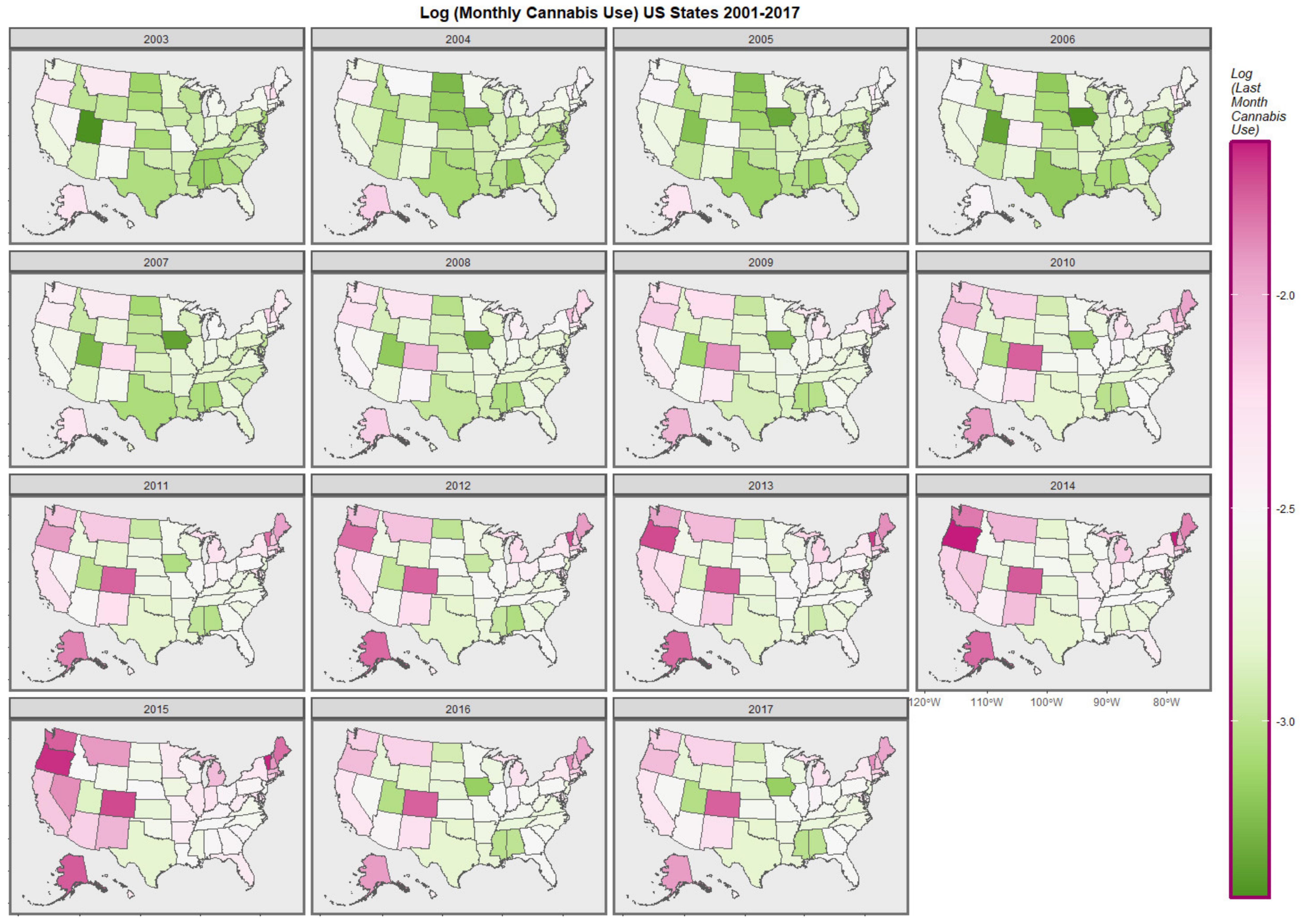
Ijerph 19 12759 g001
Figure 2. Map-graph of log(last month cannabis use rates) across USA by state and year.
Ijerph 19 12759 g002
Figure 3. Testicular cancer incidence rates by substance exposure. Substance exposure is listed as the fraction of the population reporting the applicable exposures. Median household income is reported as annual income in US dollars.
Ijerph 19 12759 g003
Figure 4. Testicular cancer incidence rates by cannabinoid exposure.
Ijerph 19 12759 g004
Figure 5. Time course of drug use across USA.
Ijerph 19 12759 g005
Figure 6. Time course of drug use across USA by cannabis legal status—scatterplots.
Ijerph 19 12759 g006
Figure 7. Substance use across USA by cannabis legal status—boxplots with aggregated time. Note that where the notches on the boxplots do not overlap this signifies a statistically significant difference.
Ijerph 19 12759 g007
Figure 8. Cannabis use and testicular cancer incidence rates by quintiles of cannabis use. (A,C) cannabis use. (B,D) testicular cancer rates. (A,B) boxplots. (C,D) scatterplots with regression lines. Note that where the notches on the boxplots do not overlap this signifies a statistically significant difference.
Ijerph 19 12759 g008
Figure 9. Cannabis use and testicular cancer incidence rates by dichotomized quintiles of cannabis use. Dichotomy contrasts highest cannabis use quintile with the lower four quintiles. (A,C) cannabis use. (B,D) testicular cancer rates. (A,B) scatterplots with regression lines. (C,D) boxplots.
Ijerph 19 12759 g009
Figure 10. Heatmap of testicular cancer rates by state. Note Hawaii near the top which is an obvious standout hotspot.
Ijerph 19 12759 g010
Figure 11. Map of geospatial neighbour links use din spatial regressions (A) edited and (B) final.
Ijerph 19 12759 g011
Figure 12. Cannabis use and testicular cancer incidence rates by cannabis legal status. (A,C) cannabis use. (B,D) testicular cancer rates. (A,B) boxplots. (C,D) scatterplots with regression lines.
Ijerph 19 12759 g012
Figure 13. Cannabis use and testicular cancer incidence rates by dichotomized cannabis legal status. Dichotomy contrasts states where cannabis is illegal vs. others. (A,C) cannabis use. (B,D) testicular cancer rates. (A,B) scatterplots with regression lines. (C,D) boxplots with notches.
Ijerph 19 12759 g013
Table 1. Introductory Linear Regressions.
Parameter EstimatesModel Parameters
Term and ModelEstimate (C.I.)p-ValueS.D.R-SquaredFdFp
lm(Rate~Time)
Year—Caucasian-Americans0.08 (0.07, 0.09)7.80 × 10−230.34520.89883741.413.20 × 10−22
Year—African Americans0.011 (−0.001, 0.024)0.09450.21840.08203.0541.220.0945
lm(Rate~mrjmon)
Cannabis0.47 (0.34, 0.59)7.50 × 10−130.59290.065253.251.7487.49 × 10−13
lm(Rate~Time * mrjmon)
Cannabis0.47 (0.34, 0.59)7.50 × 10−130.59280.065253.251.7487.50 × 10−13
Additive model
lm(Rate~Cigarettes + AUD + Cannabis + Analgesics + Cocaine)
AUD14.82 (12.14, 17.51)6.46 × 10−440.53360.242849.045.7446.46 × 10−44
Cannabis0.45 (0.32, 0.57)7.24 × 10⁻¹²
Cocaine−14.05 (−20.36, −7.74)1.45 × 10⁻⁵
Analgesics−10.22 (−14.69, −5.76)8.43 × 10⁻⁶
Cigarettes−3.19 (−4.21, −2.17)1.64 × 10⁻⁹
Quintiles
lm(Rate~Quintile)
Quintile 50.17 (0.13, 0.21)5.2 × 10−140.19270.114525.224.7451.29 × 10−19
lm(Rate~Year * Quintile)
Year0.0038 (0.0007, 0.007)0.01840.19220.119921.425.7444.66 × 10−20
Year: Quintile 50.17 (0.13, 0.21)4.21 × 10⁻¹⁴
lm(Rate~Year * Quintiles_Dichotomized)
Year0.0038 (0.0006, 0.007)0.02020.19250.116550.42.7472.94 × 10−21
Upper Quintiles0.17 (0.14, 0.21)1.37 × 10⁻²¹
Substances
lm(Rate~Substances)
Cigarettes−3.56 (−4.57, −2.55)1.04 × 10−110.59490.058747.741.7481.04 × 10−11
AUD10.61 (7.88, 13.34)8.51 × 10−140.59110.070657.851.7488.51 × 10−14
Cannabis0.47 (0.34, 0.59)7.50 × 10−130.59280.065253.251.7487.49 × 10−13
Analgesics−0.62 (−0.83, −0.41)5.42 × 10−90.59980.043234.841.7485.43 × 10−9
Cocaine−0.46 (−6.82, 5.9)8.87 × 10−10.6136−0.00130.02021.7488.87 × 10−1
Cannabinoids
lm(Rate~Cannabinoids)
THC0.25 (0.17, 0.34)6.75 × 10−90.59990.042734.391.7486.75 × 10−9
Cannabigerol0.37 (0.26, 0.48)3.55 × 10−110.59580.055745.191.7483.55 × 10−11
Cannabichromene0.45 (0.32, 0.57)1.83 × 10−120.59350.063051.381.7481.83 × 10−142
Cannabinol0.24 (0.16, 0.32)1.91 × 10−90.59890.045836.971.7481.91 × 10−9
Cannabidiol0.16 (0.06, 0.25)2.25 × 10−30.60980.01119.3971.7482.30 × 10−3
Cannabis x THC Potency0.25 (0.17, 0.34)6.75 × 10−90.60980.042734.391.7486.75 × 10−9
Legend: lm—linear modelling; Left Hand Side—Dependent Variable; Right Hand side—List of independent covariates; ~—Separator between left and right hand sides of a model formula; +—Additive relationship between covariates; *—Interactive relationship between covariates—includes additive relationships; AUD-Alcohol Use Disorder.
Table 2. Mixed Effects Regressions.
Parameter EstimatesModel Parameters
ParameterEstimate (C.I.)p-ValueS.D.AICBICLoglik
Cannabis Alone—Race as Random Effects
lme(Testicular_Cancer_Rate~Cannabis)
Cannabis0.16 (0.15, 0.18)1.70 × 10−750.1972−1816.237−1790.591912.1183
Additive Model
lme(Testicular_Cancer_Rate~Cigarettes + AUD + Cannabis + Analgesics + Cocaine)
AUD4.96 (4.59, 5.32)3.01 × 10−1460.1764−2802.042−2750.7581409.021
Cannabis0.15 (0.14, 0.17)1.14 × 10−68
Cocaine−4.23 (−5.09, −3.38)3.72 × 10⁻²²
Analgesics−0.16 (−0.19, −0.13)9.53 × 10⁻³¹
Cigarettes−1.07 (−1.21, −0.93)2.96 × 10−50
3-Way Interactive Model
lme(Testicular_Cancer_Rate~Cigarettes * AUD * Cannabis + Analgesics + Cocaine)
Cigarettes: Cannabis11.07 (9.32, 12.82)1.03 × 10−340.1695−3172.38−3095.4651598.19
Cigarettes27.64 (22.84, 32.44)3.84 × 10⁻²⁹
AUD64.33 (48.44, 80.22)2.64 × 10⁻¹⁵
Cannabis: AUD23.66 (17.76, 29.55)4.40 × 10⁻¹⁵
Cocaine−2.75 (−3.6, −1.89)3.43 × 10⁻¹⁰
Cigarettes: AUD−293.19 (−361.6, −224.77)5.95 × 10⁻¹⁷
Cigarettes: Cannabis: AUD−115.24 (−140.38, −90.09)3.82 × 10⁻¹⁹
Cannabis−2.14 (−2.54, −1.74)1.57 × 10⁻²⁵
Analgesics−0.15 (−0.18, −0.12)3.76 × 10⁻²⁹
4-Way Interactive Model
lme(Testicular_Cancer_Rate~Cigarettes * AUD * Cannabis * Analgesics + Cocaine)
Cannabis: Analgesics2.08 (1.64, 2.51)9.32 × 10−210.1684−3212.364−3116.231621.182
Analgesics5.44 (4.3, 6.58)1.12 × 10⁻²⁰
Cigarettes: Cannabis: AUD: Analgesics33.83 (25.81, 41.85)1.78 × 10⁻¹⁶
Cigarettes: AUD: Analgesics85.86 (63.96, 107.76)1.87 × 10⁻¹⁴
Cannabis4.4 (3.09, 5.71)4.51 × 10⁻¹¹
Cocaine−1.94 (−2.8, −1.07)1.15 × 10−05
Cigarettes: Cannabis−20.18 (−26.02, −14.34)1.41 × 10⁻¹¹
Cannabis: AUD: Analgesics−6.68 (−8.56, −4.79)4.30 × 10⁻¹²
Cigarettes−55.44 (−71.02, −39.86)3.54 × 10⁻¹²
AUD: Analgesics−18.32 (−23.42, −13.22)2.14 × 10⁻¹²
Cigarettes: Analgesics−26.55 (−31.79, −21.31)4.98 × 10⁻²³
Cigarettes: Cannabis: Analgesics−9.99 (−11.95, −8.02)3.75 × 10⁻²³
4-Way Interactive Model with Income
lme(Testicular_Cancer_Rate~Cigarettes * AUD * Cannabis * Analgesics + Cocaine + Income)
Analgesics5.46 (4.33, 6.59)5.04 × 10−210.1674−3258.286−3155.7471645.143
Cannabis: Analgesics2.04 (1.61, 2.47)3.17 × 10⁻²⁰
Cigarettes: Cannabis: AUD: Analgesics34.58 (26.61, 42.56)2.57 × 10⁻¹⁷
Cigarettes: AUD: Analgesics87.71 (65.94, 109.49)3.63 × 10⁻¹⁵
log(MHY)0.16 (0.12, 0.21)2.38 × 10⁻¹³
Cannabis4.25 (2.95, 5.54)1.70 × 10⁻¹⁰
Cocaine−2.15 (−3.01, −1.29)1.08 × 10⁻⁶
Cigarettes: Cannabis−20.22 (−26.03, −14.42)9.74 × 10⁻¹²
Cigarettes−56.6 (−72.1, −41.11)9.34 × 10⁻¹³
Cannabis: AUD: Analgesics−6.91 (−8.78, −5.04)5.83 × 10⁻¹³
AUD: Analgesics−18.86 (−23.93, −13.79)3.56 × 10⁻¹³
Cigarettes: Cannabis: Analgesics−10 (−11.95, −8.04)1.96 × 10⁻²³
Cigarettes: Analgesics−27.04 (−32.25, −21.83)4.60 × 10⁻²⁴
Legend: See Table 1. lme—Mixed effects regressions; A.I.C.—Akaike Information Criterion; B.I.C.—Bayesian Information Criterion; logLik—Log of the Maximum Likelihood Ratio at model optimization; *—interaction term between covariates.
Table 3. Robust Inverse Probability Weighted Regressions.
ParameterEstimate (C.I.)p-Value
Additive Model with State Cannabis
svyglm(TestCaRt~Cigarettes + Cannabis + Race + AUD + Analgesics + Cocaine)
AUD64.55 (56.89, 72.22)<2.2 × 10⁻¹⁶
Analgesics11.01 (6.24, 15.77)5.7 × 10⁻⁵
NHWhite5.44 (2.36, 8.53)0.0013
Hispanic4.63 (1.54, 7.71)0.0055
Cannabis−9.38 (−12.76, −5.99)3.4 × 10⁻⁶
Cocaine−131.14 (−138.96, −123.33)<2.2 × 10⁻¹⁶
Additive Model with Ethnic THC Exposure
svyglm(TestCaRt~Cigarettes * EthnicTHCExposure * Race + AUD + Analgesics + Cocaine)
Cigarettes28.96 (27.87, 30.05)<2 × 10⁻¹⁶
Hispanic2.55 (2.05, 3.04)1.8 × 10⁻¹²
Asian4.89 (1.08, 8.69)0.0160
EthnicTHCExposure2.9 (0.41, 5.38)0.0281
Cocaine−56.03 (−110.14, −1.93)0.0492
Interactive Model with Ethnic_THC_Exposure
svyglm(TestCaRt~Cigarettes * EthnicTHCExposure * Race + AUD + Analgesics + Cocaine + Income)
EthnicTHCExposure4.72 (2.04, 7.41)0.0018
Asian3.93 (1.64, 6.22)0.0022
Cigarettes11.09 (3.77, 18.42)0.0060
Cigarettes: NHWhite109.87 (24.24, 195.5)0.0177
Cigarettes: EthnicTHCExposure: Asian17.32 (1.64, 33.01)0.0388
NHWhite−19.53 (−39.11, 0.05)0.0603
EthnicTHCExposure: Asian−4.45 (−8.41, −0.5)0.0352
Cocaine−88.11 (−161.51, −14.7)0.0257
Cigarettes: EthnicTHCExposure−20.11 (−32.44, −7.78)0.0034
Cigarettes: Asian−16.35 (−26.11, −6.6)0.0027
Interactive Model with State Cannabis
svyglm(TestCaRt~Cigarettes * Cannabis * Race + AUD + Analgesics + Cocaine + Income)
AUD13.58 (7.69, 19.47)0.0001
Cigarettes: Cannabis: NHWhite398.68 (214.58, 582.79)0.0002
Cigarettes: NHWhite933.24 (493.05, 1373.44)0.0003
Cigarettes: Hispanic1372.45 (672.78, 2072.11)0.0007
Cigarettes: Cannabis: Hispanic635.8 (305.36, 966.24)0.0008
Analgesics19.88 (9.19, 30.57)0.0011
Cannabis42.63 (18.65, 66.61)0.0017
Cigarettes: Cannabis−199.68 (−315.91, −83.44)0.0023
Cigarettes−578.67 (−907.11, −250.23)0.0018
Cocaine−75.51 (−117.23, −33.78)0.0015
Cannabis: Hispanic−144.06 (−218.53, −69.59)0.0008
Hispanic−308.36 (−466.63, −150.09)0.0007
NHWhite−214 (−315.14, −112.87)0.0003
Cannabis: NHWhite−93.06 (−135.37, −50.75)0.0002
Interactive Model with State Cannabinoids
svyglm(TestCaRt~Cigarettes * THC * Cannabigerol * Race + AUD + Analgesics + Cocaine + Income)
Cigarettes: NHWhite127.24 (92.37, 162.1)4.7 × 10⁻⁷
Cigarettes: THC: Cannabigerol: NHBlack13.87 (6.33, 21.41)0.0017
Cigarettes: NHBlack53.77 (18.14, 89.41)0.0075
Cigarettes: THC: NHBlack49.95 (14.93, 84.96)0.0108
Cigarettes: Cannabigerol: NHBlack14.62 (3.67, 25.57)0.0161
Cigarettes: THC: Cannabigerol: NHWhite35.97 (7.97, 63.97)0.0200
Cigarettes: THC: Hispanic214.68 (31.83, 397.53)0.0317
Cigarettes: Hispanic−310.38 (−540.45, −80.31)0.0152
Cigarettes: Cannabigerol: Hispanic−89.37 (−155.46, −23.28)0.0150
AUD−43.07 (−68.76, −17.38)0.0035
THC: Cannabigerol: NHWhite−8.18 (−11.39, −4.96)6.2 × 10⁻⁵
NHWhite−16.98 (−23.16, −10.81)2.4 × 10⁻⁵
Legend: See Table 1. Svyglm—Robust generalized linear regression; TestCaRt—Testicular Cancer Rate; *—interaction term between covariates.
Table 4. Geospatiotemporal Regressions.
Lagged VariablesParameterModel
ParameterEstimate (C.I.)p-ValueLogLikS.D.Model ParameterEstimatep-Value
spreml(Rate~Cannabis) phi1.29101.4 × 10−5
Cannabis0.19 (0.1, 0.28)3.4 × 10⁻⁵−390.89630.3939psi−0.11140.0055
rho−0.37950.0055
lambda0.42982.1 × 10−5
spreml(Rate~Cigarettes + AUD + Cannabis + Analgesics + Cocaine)
phi1.29101.4 × 10−5
Cannabis0.19 (0.1, 0.28)3.4 × 10⁻⁵−390.86930.5316psi−0.11140.0055
rho−0.37950.0055
lambda0.42982.1 × 10−5
spreml(Rate~Cigarettes * Cannabis * AUD + Analgesics + Cocaine)
phi1.26502.6 × 10−5
Cigarettes: Cannabis0.36 (0.19, 0.53)4.6 × 10⁻⁵−391.16680.5300psi−0.11010.0062
rho−0.36960.0088
lambda0.42425.2 × 10−5
spreml(Rate~Cigarettes * Cannabis * AUD + Analgesics + Cocaine + Income + 5_Races)
CaucAsian-Am.1.59 (1.26, 1.93)<2.2 × 10⁻¹⁶−353.35390.1584phi0.18460.0004
Hispanic-Am.0.1 (0.03, 0.16)6.0 × 10⁻³ psi−0.08910.0284
Asian-Am.0.13 (0.07, 0.2)8.3 × 10⁻⁵ rho−0.17660.2595
African-Am.−0.23 (−0.27, −0.19)<2.2 × 10⁻¹⁶ lambda0.21830.0847
spreml(Rate~Cigarettes * THC * Cannabigerol * AUD + Analgesics + Cocaine + Income + 5_Races)
CaucAsian-Am.1.6 (1.16, 2.03)8.0 × 10⁻¹³−348.34280.3929phi0.15720.0009
Hispanic-Am.0.11 (0.04, 0.18)0.0028 psi−0.09550.0197
Asian-Am.0.11 (0.03, 0.19)0.0074 rho−0.16420.1982
Cigarettes: Cannabigerol1.39 (0.24, 2.53)0.0177 lambda0.19450.0531
THC: Cannabigerol0.07 (0.01, 0.12)0.0187
Cigarettes4.45 (0.34, 8.56)0.0340
Analgesics−0.18 (−0.36, 0)0.0457
African-Am.−0.22 (−0.26, −0.17)<2.2 × 10⁻¹⁶
2 Spatial Lags
spreml(Rate~Cigarettes * THC * Cannabigerol * AUD + Analgesics + Cocaine + Income + 5_Races)
CBG, 2Caucasian-Am.1.63 (1.18, 2.08)1.2 × 10⁻¹²−351.1620.3970phi0.18820.0004
Asian-Am.0.14 (0.06, 0.22)0.0007 psi−0.09760.0167
Hispanic-Am.0.1 (0.03, 0.17)0.0054 rho−0.18250.2500
Cigarettes: THC: Cannabigerol0.71 (0.05, 1.37)0.0350 lambda0.21990.0845
Cigarettes: THC2.58 (0.17, 4.98)0.0356
African-Am.−0.23 (−0.27, −0.19)<2.2 × 10⁻¹⁶
2 Temporal Lags
spreml(Rate~Cigarettes * THC * Cannabigerol * AUD + Analgesics + Cocaine + Income + 5_Races)
CBG, 2Caucasian-Am.1.8 (1.33, 2.26)4.6 × 10⁻¹⁴−294.76630.3863phi0.14870.0012
Asian-Am.0.16 (0.08, 0.23)5.2 × 10⁻⁵ psi−0.09720.0289
Hispanic-Am.0.15 (0.07, 0.22)7.3 × 10⁻⁵ rho−0.17700.2840
Cigarettes: THC23.6 (11.92, 35.29)7.5 × 10⁻⁵ lambda0.20250.1205
Cigarettes: THC: Cannabigerol6.22 (3.07, 9.37)0.0001
Cannabigerol0.18 (0.04, 0.32)0.0146
Analgesics−0.27 (−0.44, −0.09)0.0031
THC: Cannabigerol−1.26 (−1.94, −0.57)0.0003
THC−4.86 (−7.36, −2.37)0.0001
African-Am.−0.22 (−0.26, −0.18)<2.2 × 10⁻¹⁶
Full Model with Ethnic THC Exposure
spreml(Rate~Cigarettes * AUD + Analgesics + Cocaine + MHY + NHCaucasian-Am._THC_Exposure * NHAfrican-Am._THC_Exposure * Hispanic-Am._THC_Exposure + Asian-Am._THC_Exposure + AIAN_THC_Exposure)
NHAfrican-Am._THC_Exposure0.15 (0.06, 0.25)0.0009−380.05120.4856phi1.00871.1 × 10−5
Asian-Am._THC_Exposure−0.1 (−0.19, −0.02)0.0173 psi−0.11420.0044
rho−0.51613.9 × 10−8
lambda0.47204.4 × 10−13
Legend: See Table 1. Spreml—Spatial Panel Random Effects Maximum Likelihood Regression; 5_Races—Caucasian- African- Hispanic- Asian- American Indian/Alaskan Native- American ancestry; phi—Random error coefficient; psi—Serial correlation coefficient; rho—Spatial error coefficient; lambda—Spatial error autocorrelation coefficient; * interaction term between covariates.
Table 5. Selected e-Values.
ParameterEstimate (C.I.)R.R. (C.I.)E-Values
LINEAR MODELS
Testicular_Cancer~Cannabis
Cannabis0.47 (0.34, 0.59)2.04 (1.69, 2.47)3.50, 2.76
Testicular_Cancer~Time * Cannabis
Cannabis0.47 (0.34, 0.59)2.04 (1.68, 2.47)3.50, 2.76
Additive Drug Model
Cannabis0.45 (0.32, 0.57)2.14 (1.73, 2.65)3.70, 2.85
Testicular_Cancer~Cannabis Quintiles
Quintile 50.17 (0.13, 0.21)2.13 (1.75, 2.58)3.68, 2.91
Testicular_Cancer~Time * Cannabis_Quintiles
Year: Quintile 50.17 (0.13, 0.21)2.23 (1.82, 2.73)3.88, 3.04
Testicular_Cancer~Time * Dichotomized_Cannabis_Quintiles
Upper Quintiles0.17 (0.14, 0.21)2.24 (1.91, 2.64)3.91, 3.22
Substances
Cannabis0.47 (0.34, 0.59)2.04 (122.69, 2.43)3.50, 2.76
THC0.25 (0.17, 0.34)1.47 (1.29, 1.67)2.30, 1.91
Cannabigerol0.37 (0.26, 0.48)1.76 (1.49, 2.08)2.92, 2.35
Cannabichromene0.45 (0.32, 0.57)1.98 (1.64, 2.39)3.38, 2.68
Cannabinol0.24 (0.16, 0.32)1.43 (1.27, 1.61)2.23, 1.88
Cannabidiol0.16 (0.06, 0.25)1.26 (1.08, 1.46)1.83, 1.40
Cannabis x THC Potency0.25 (0.17, 0.34)1.46 (1.28, 1.66)2.28, 1.90
MIXED EFFECTS
Cannabis Alone—Race as Random Effects
Cannabis0.16 (0.15, 0.18)3.51 (3.08, 4.00)6.48, 5.61
Additive Model
Cannabis0.15 (0.14, 0.17)3.29 (2.89, 3.76)6.05, 5.23
3-Way Interactive Model
Cigarettes: Cannabis11.07 (9.32, 12.82)9.67 × 1025 (7.66 × 10²¹, 1.22 × 1030)1.95 × 1026, 1.54 × 10²²
Cannabis: AUD23.66 (17.76, 29.55)3.23 × 1055 (5.17 × 1041, 2.02 × 1069)6.45 × 1055, 1.03 × 1042
4-Way Interactive Model
Cannabis: Analgesics2.08 (1.64, 2.51)7.48 × 10⁴ (7.22 × 10³, 7.75 × 10⁵)1.49 × 10⁵, 1.44 × 10⁴
Cigarettes: Cannabis: AUD: Analgesics33.83 (25.81, 41.85)2.41 × 1079 (4.00 × 1060, 1.46 × 1098)4.84 × 1079, 8.01 × 1060
Cannabis4.4 (3.09, 5.71)2.13 × 10¹⁰ (1.85 × 10⁸, 2.45 × 10¹³)4.26 × 10¹⁰, 3.71 × 10⁸
4-Way Interactive Model with Income
Cannabis: Analgesics2.04 (1.61, 2.47)6.41 × 10⁴ (6.18 × 10³, 6.64 × 10⁵)1.28 × 10⁵, 1.24 × 10⁴
Cigarettes: Cannabis: AUD: Analgesics34.58 (26.61, 42.56)4.31 × 1081 (7.03 × 1062, 2.64 × 10100)8.61 × 1081, 1.40 × 1063
Cannabis4.25 (2.95, 5.54)1.05 × 10¹⁰ (9.08 × 10⁶, 1.21 × 10¹³)2.09 × 10¹⁰, 1.82 × 10⁷
GEOSPATIAL MODELS
spreml(Rate~Cannabis)
Cannabis0.19 (0.1, 0.28)1.55 (1.18, 2.05)2.48, 1.64
spreml(Rate~Cigarettes + AUD + Cannabis + Analgesics + Cocaine)
Cannabis0.19 (0.1, 0.28)1.39 (1.19, 1.62)2.12, 1.66
spreml(Rate~Cigarettes * Cannabis * AUD + Analgesics + Cocaine)
Cigarettes: Cannabis0.36 (0.19, 0.53)1.85 (1.38, 2.49)3.11, 2.10
spreml(Rate~Cigarettes * THC * Cannabigerol * AUD + Analgesics + Cocaine + Income + 5_Races)
Cigarettes: Cannabigerol1.39 (0.24, 2.53)24.77 (1.76, 349.61)49.05, 2.91
THC: Cannabigerol0.07 (0.01, 0.12)1.16 (1.03, 1.32)1.60, 1.19
2 Spatial Lags
Cigarettes: THC: Cannabigerol0.71 (0.05, 1.37)5.09 (1.12, 23.10)9.66, 1.50
Cigarettes: THC2.58 (0.17, 4.98)368.56 (1.51, 9.02 × 10⁴)736.63, 2.38
2 Temporal Lags
Cigarettes: THC23.6 (11.92, 35.29)1.40 × 1024 (1.64 × 10¹², 1.20 × 1036)2.81 × 1024, 3.29 × 10¹²
Cigarettes: THC: Cannabigerol6.22 (3.07, 9.37)2.31 × 10⁶ (1.39 × 10³, 3.82 × 10⁹)4.62 × 10⁶, 2.79 × 10³
Cannabigerol0.18 (0.04, 0.32)1.52 (1.09, 2.13)2.41, 1.39
spreml(Rate~Cigarettes * AUD + Analgesics + Cocaine + MHY + NHCaucasian-Am._THC_Exposure * NHAfrican-Am._THC_Exposure * Hispanic-Am._THC_Exposure + Asian-Am._THC_Exposure + AIAN_THC_Exposure)
NHAfrican-Am._THC_Exposure0.15 (0.06, 0.25)1.33 (1.13, 1.58)2.00, 1.51
LEGAL STATUS
Legal0.14 (0.06, 0.22)1.88, (1.33, 2.66)3.16, 1.98
Medical0.05 (0.01, 0.09)1.25 (1.06, 1.48)1.82, 1.31
Legal Status Over Time
Legal0.11 (0.03, 0.19)1.63 (1.12, 2.34)2.63, 1.50
Dichotomized Status
Liberal0.05 (0.02, 0.08)1.25 (1.10, 1.43)1.81, 1.43
Dichotomized Status Over Time
Liberal0.05 (0.02, 0.08)1.25 (1.10, 1.43)1.81, 1.43
Quintiles
Quintile 50.20 (0.13, 0.21)2.13 (1.75, 2.58)3.68, 2.91
Dichotomized Quintiles
Upper_2_Quintiles0.20 (0.06, 0.35)2.24 (1.91, 2.64)3.91, 3.22
Abbreviations: R.R.—Relative Risk. * interaction term between covariates.
Table 6. Ordered e-Value Lists.
No.E-Value EstimatesMinimum E-Value
18.61 × 10811.40 × 1063
24.84 × 10798.01 × 1060
36.45 × 10551.03 × 1042
41.95 × 10261.54 × 1022
52.81 × 10243.29 × 1012
64.26 × 10103.71 × 108
72.09 × 10101.82 × 107
84.62 × 10614,400.00
91.49 × 10512,400.00
101.28 × 1052790.00
11736.635.61
1249.055.23
139.663.22
146.483.22
156.053.04
163.912.91
173.912.91
183.882.91
193.702.85
203.682.76
213.682.76
223.502.76
233.502.68
243.502.38
253.382.35
263.162.10
273.111.98
282.921.91
292.631.9
302.481.88
312.411.66
322.301.64
332.281.51
342.231.50
352.121.50
362.001.43
371.831.43
381.821.40
391.811.39
401.811.31
411.601.19
Table 7. Effect of Cannabis Legalization.
Linear Models
Parameter EstimatesModel Parameters
ParameterEstimate (C.I.)p-ValueS.D.R-SquaredFdFp
Legal Status
(lm(Rate~Status)
Decriminalized0.03 (−0.01, 0.07)0.09790.20290.01965.9793.7460.0005
Legal0.14 (0.06, 0.22)0.0004
Medical0.05 (0.01, 0.09)0.0086
(lm(Rate~Year * Status)
Legal0.11 (0.03, 0.19)0.01020.20291.96 × 10−25.9793.7460.0005
(lm(Rate~Dichotomized Status)
Liberal0.05 (0.02, 0.08)0.00080.20350.013511.241.7480.0008
(lm(Rate~Year * Dichotomized Status)
Liberal0.05 (0.02, 0.08)0.00080.20350.013511.241.7480.0008
Linear Models from Imputed Dataset
ParametersModel
ParameterEstimate (C.I.)p-ValueNo. ImputationsSDlambdaFMI
From Imputed Dataset
Dichotomized Quintiles
lm(TestCaRt~Dichotomized_Quintiles)
Upper_2_Quintiles0.20 (0.06, 0.35)0.00582561.83750.03090.0316
Abbreviations: FMI—Fraction of missing information; Lambda—Proportion of information which is due to missing data; * interaction term.
Publisher’s Note: MDPI stays neutral with regard to jurisdictional claims in published maps and institutional affiliations.

