

Analysis of Vertical Distribution Changes and Influencing Factors of Tropospheric Ozone in China from 2005 to 2020 Based on Multi-Source Data


Abstract
:1. Introduction
2. Data and Methods
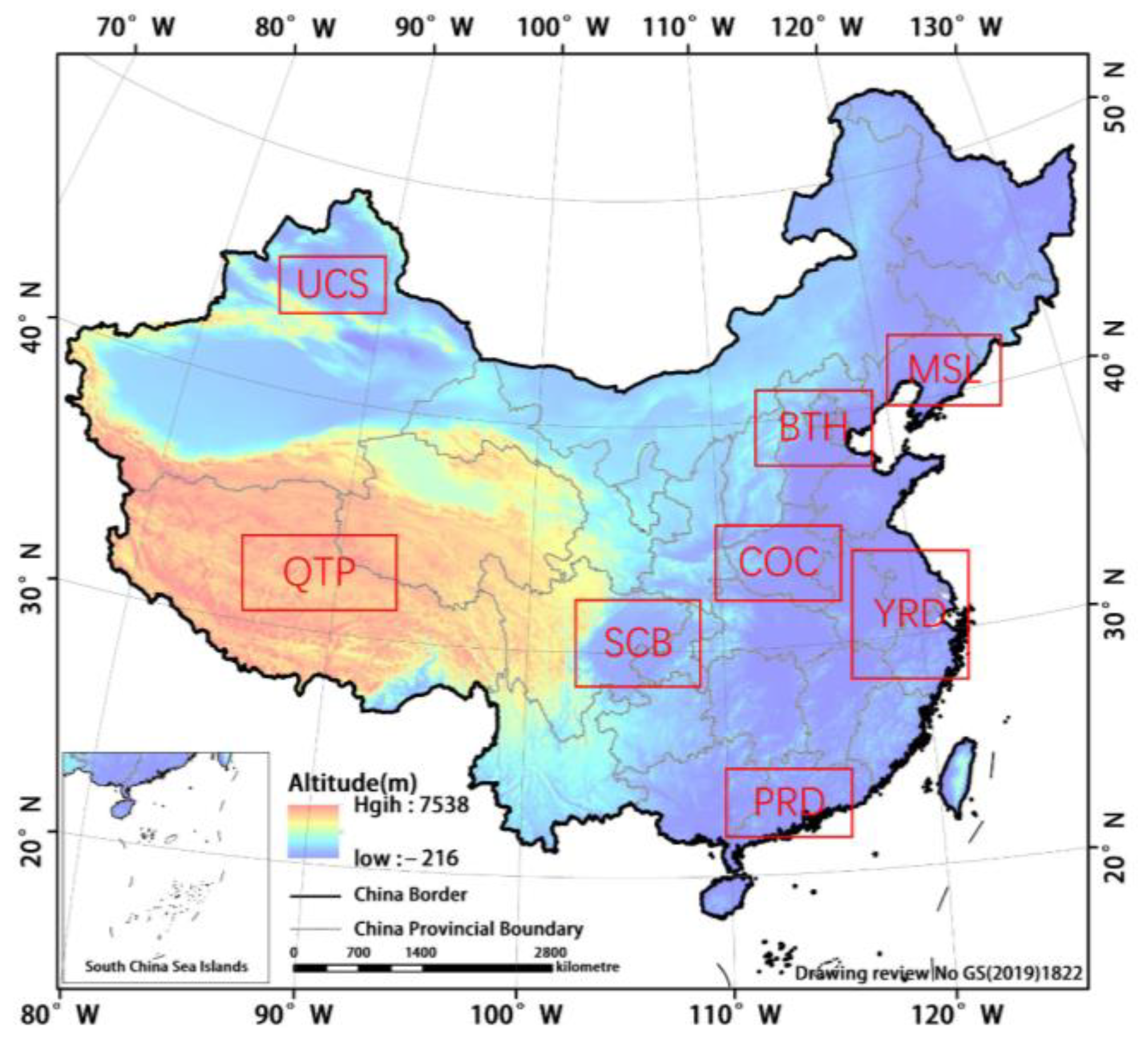
2.1. Overview of the Study Area
2.2. Data Introduction
2.3. Research Methodology
2.3.1. Data Pre-Processing
2.3.2. Statistical Analysis
3. Results and Analysis
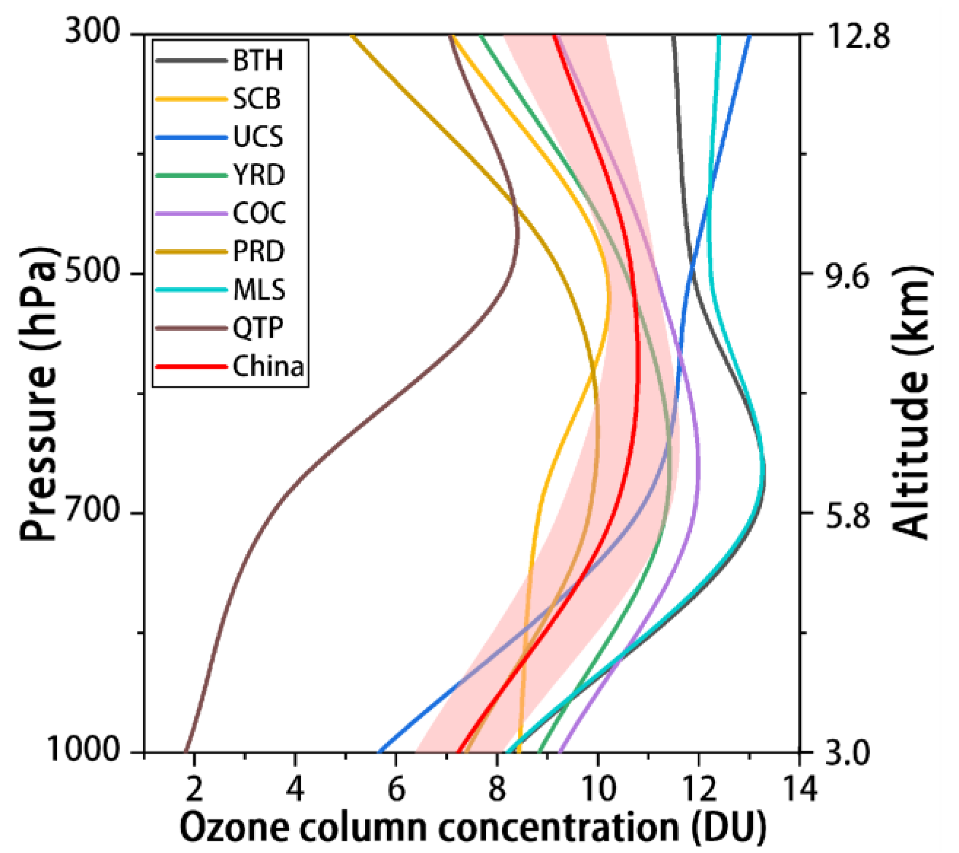
3.1. Characteristics of the Vertical Spatial Distribution of Tropospheric Ozone
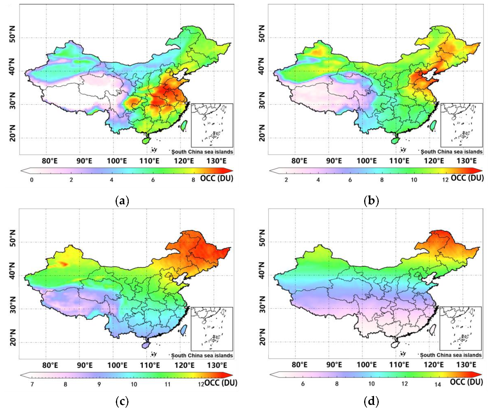
3.1.1. Characteristics of the Horizontal Distribution of Tropospheric Ozone at Different Heights
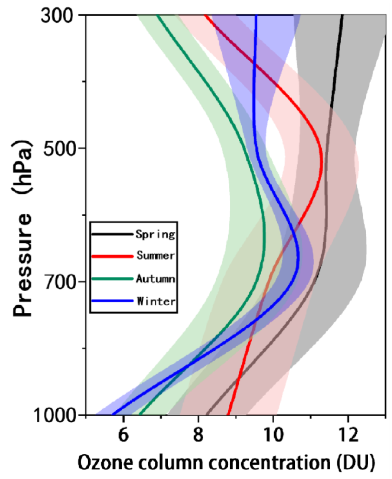
3.1.2. Seasonal Distribution Characteristics of Tropospheric Ozone at Different Heights
3.2. Time-Varying Characteristics of the Vertical Profile of Tropospheric Ozone
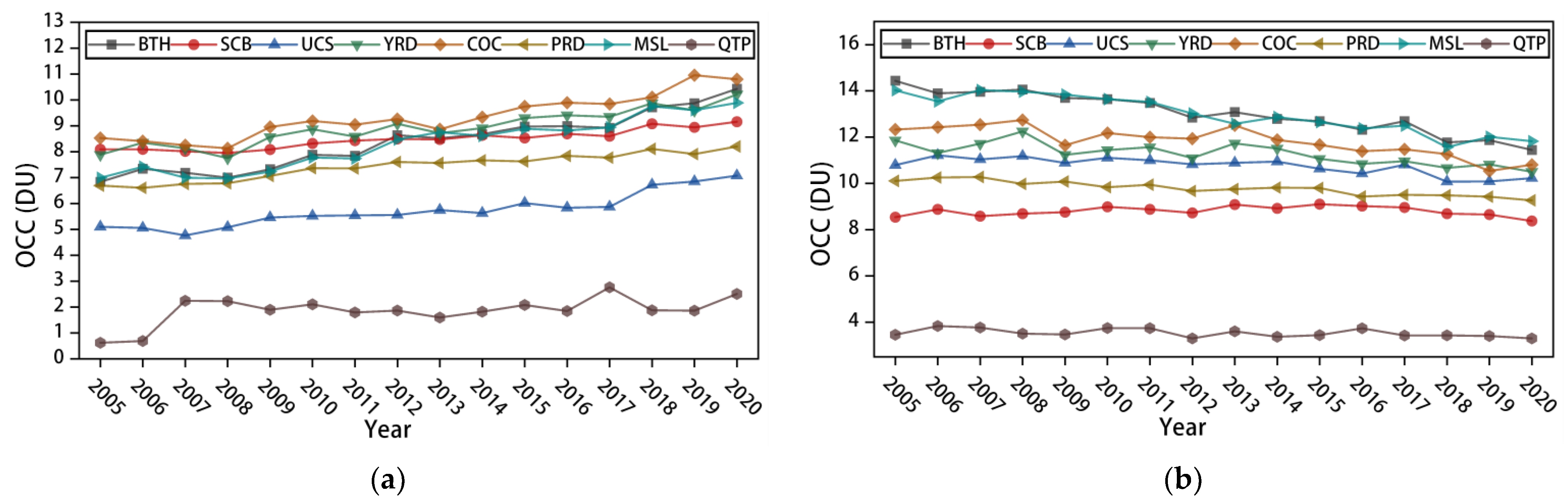
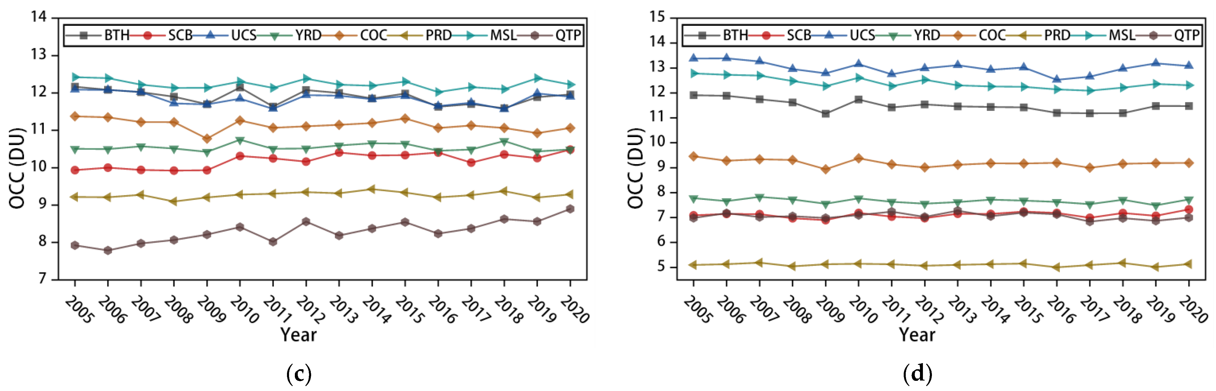
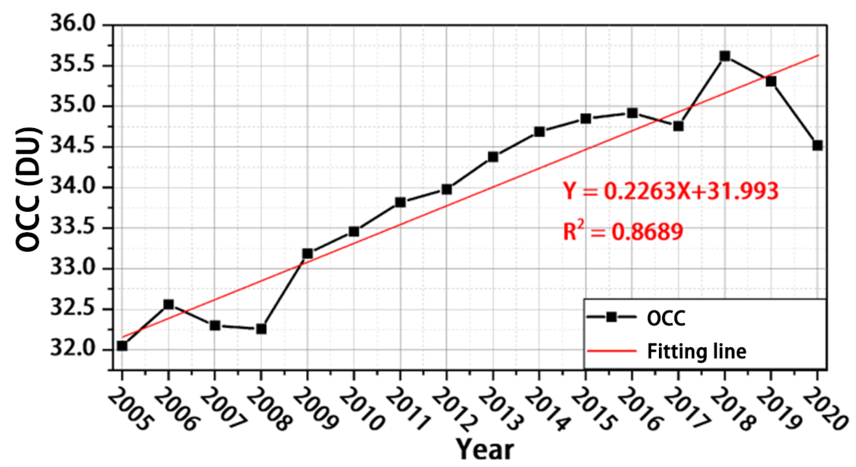
3.2.1. Characteristics of Interannual Variability
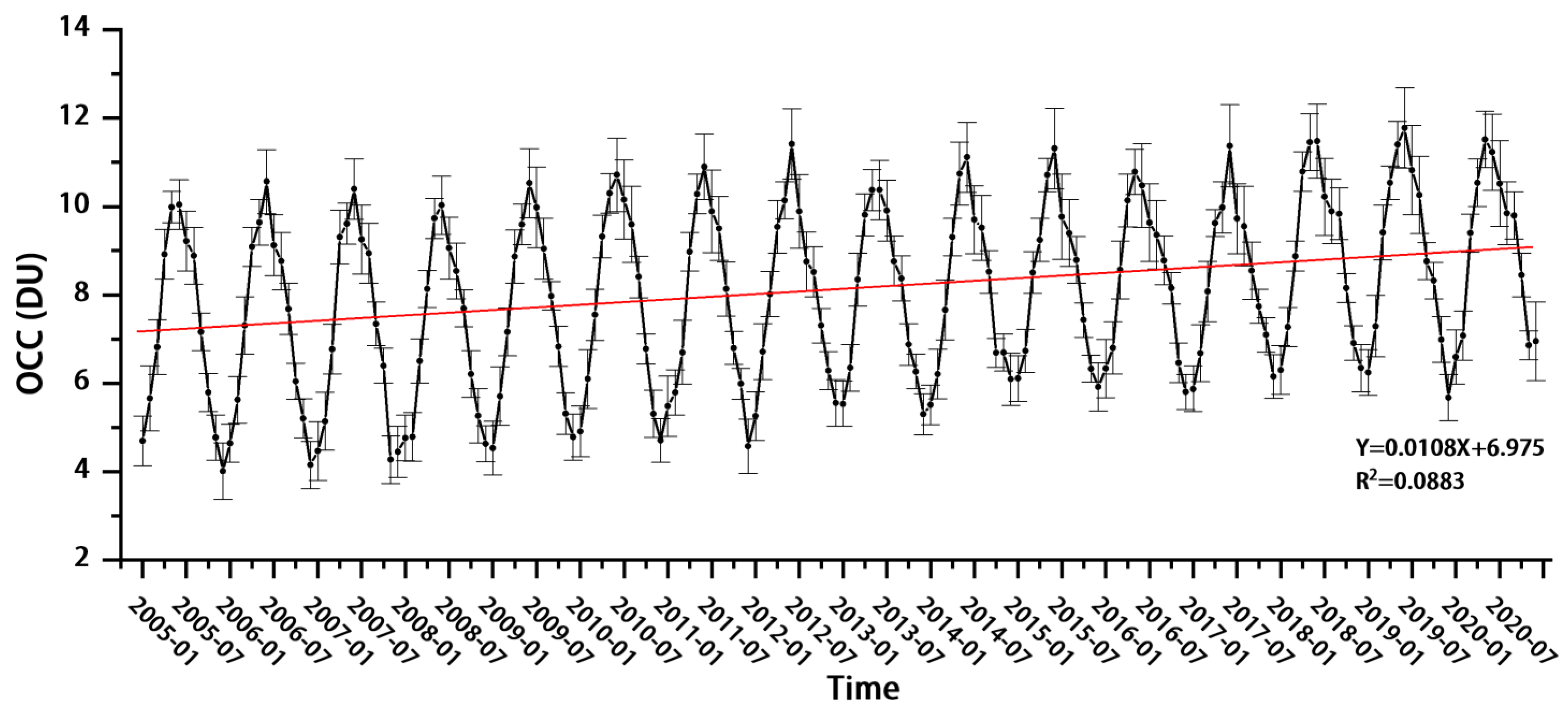
3.2.2. Characteristics of Monthly Variation
4. Discussion
4.1. Ozone Transport in the 3–5.8 km Altitude Layer
4.2. Precursor Effects
4.3. Vegetation Growth Effects
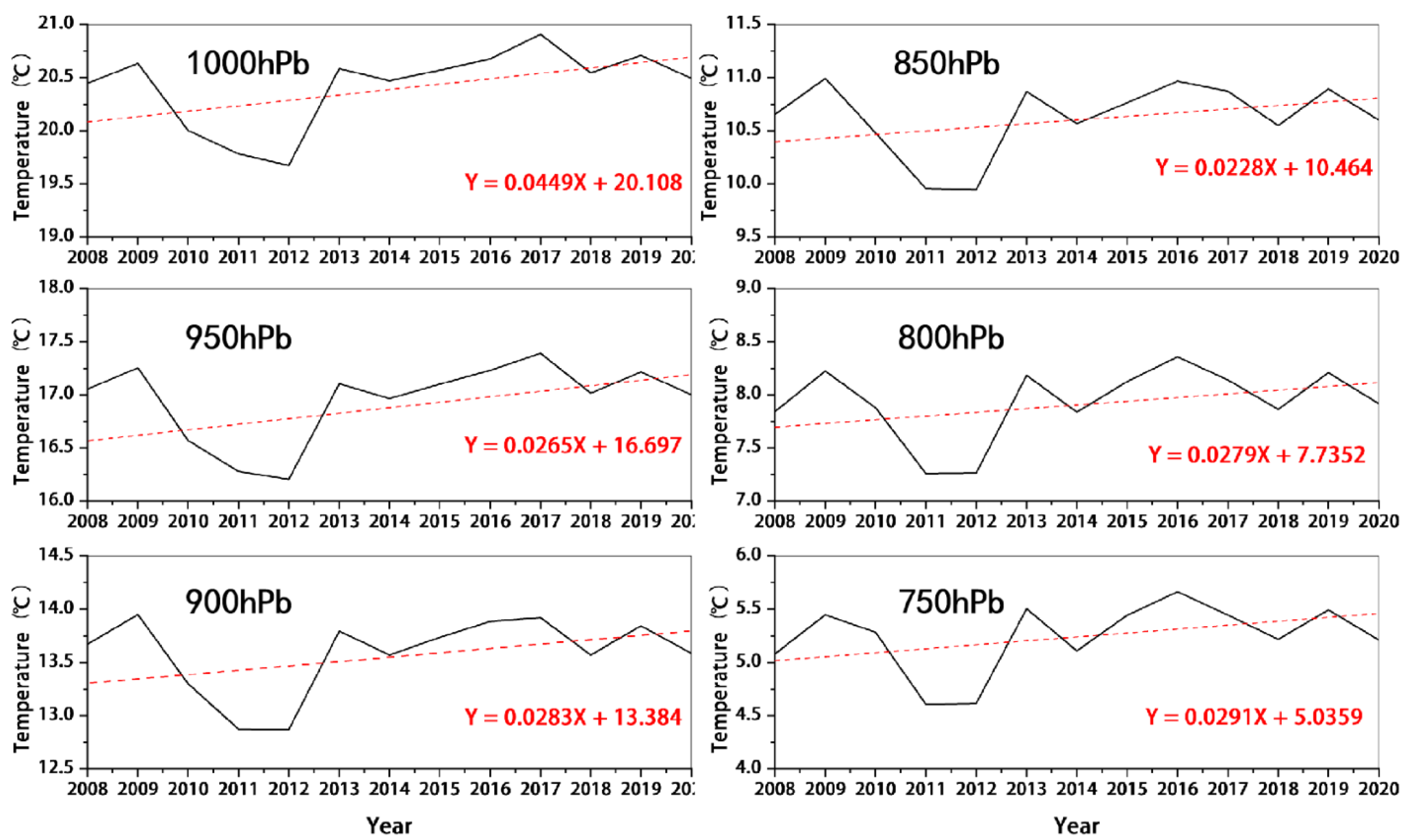
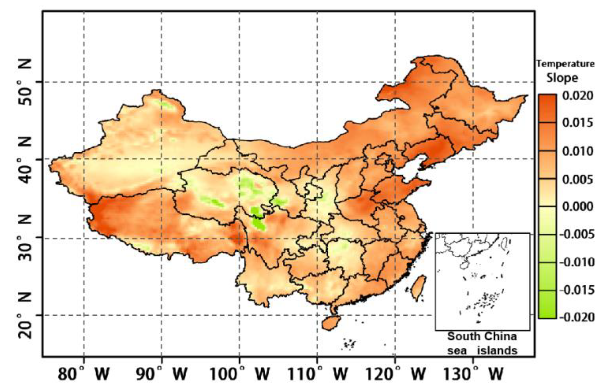
4.4. Temperature Effect
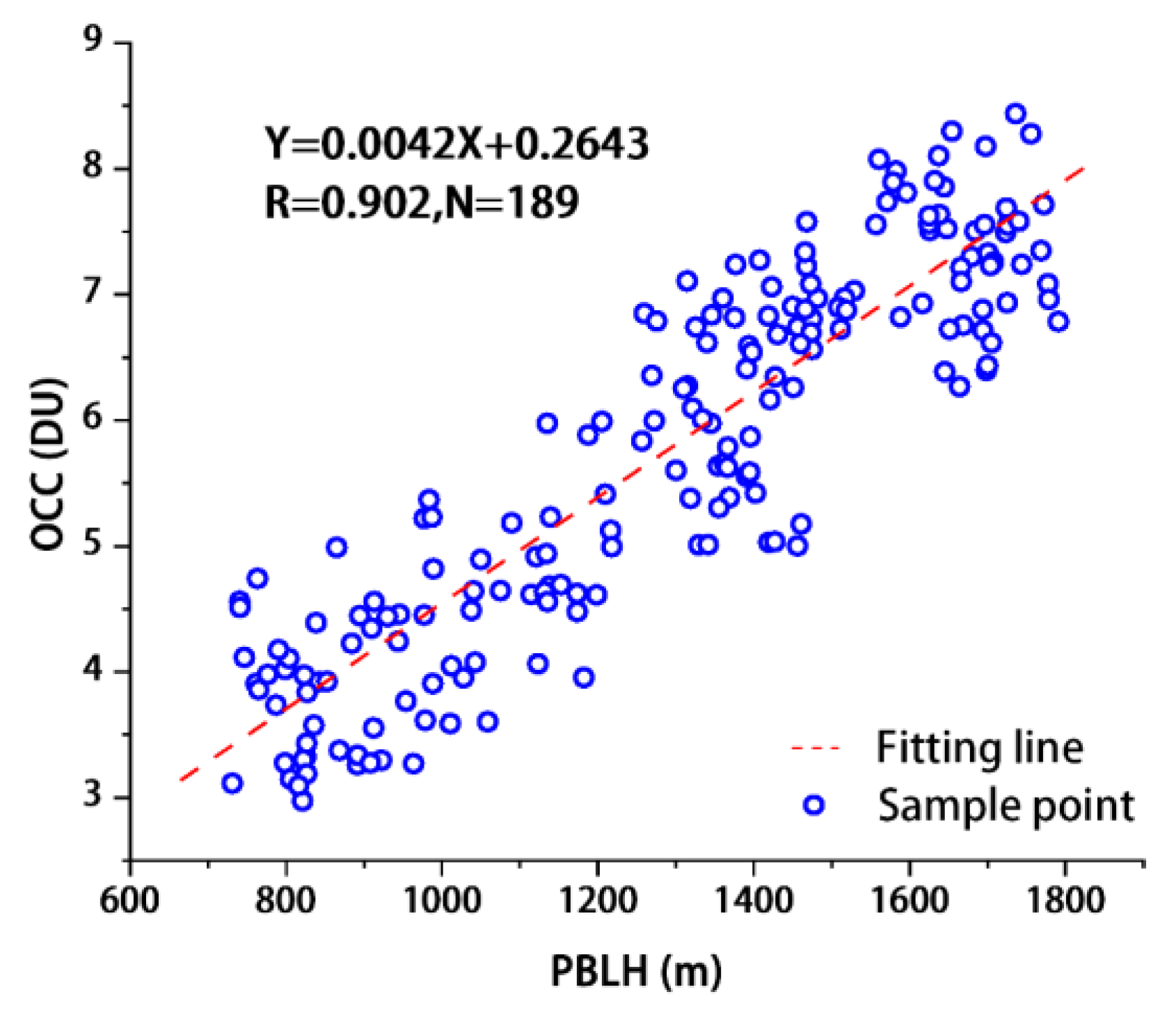
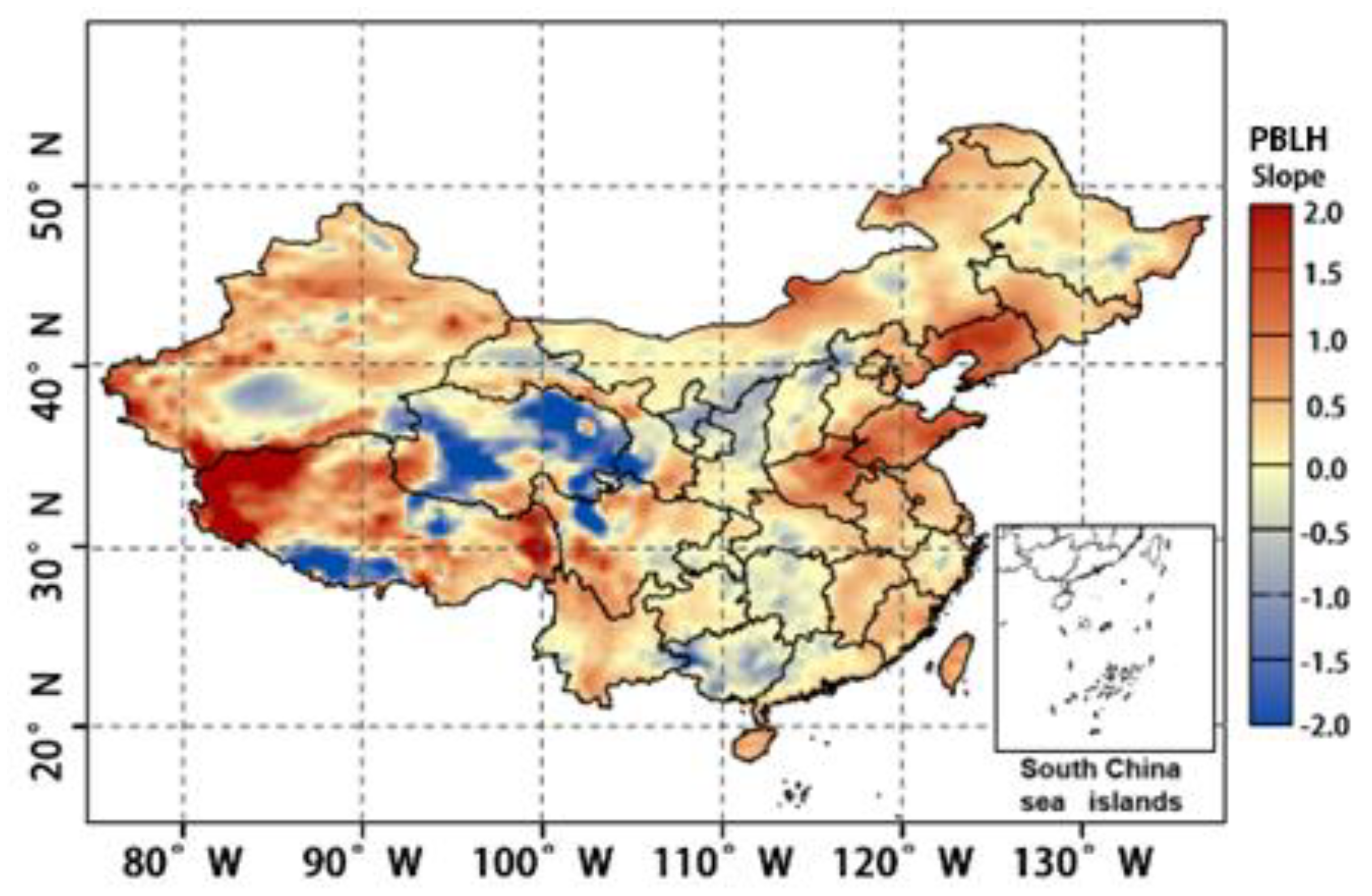
4.5. PBLH Effects
5. Conclusions
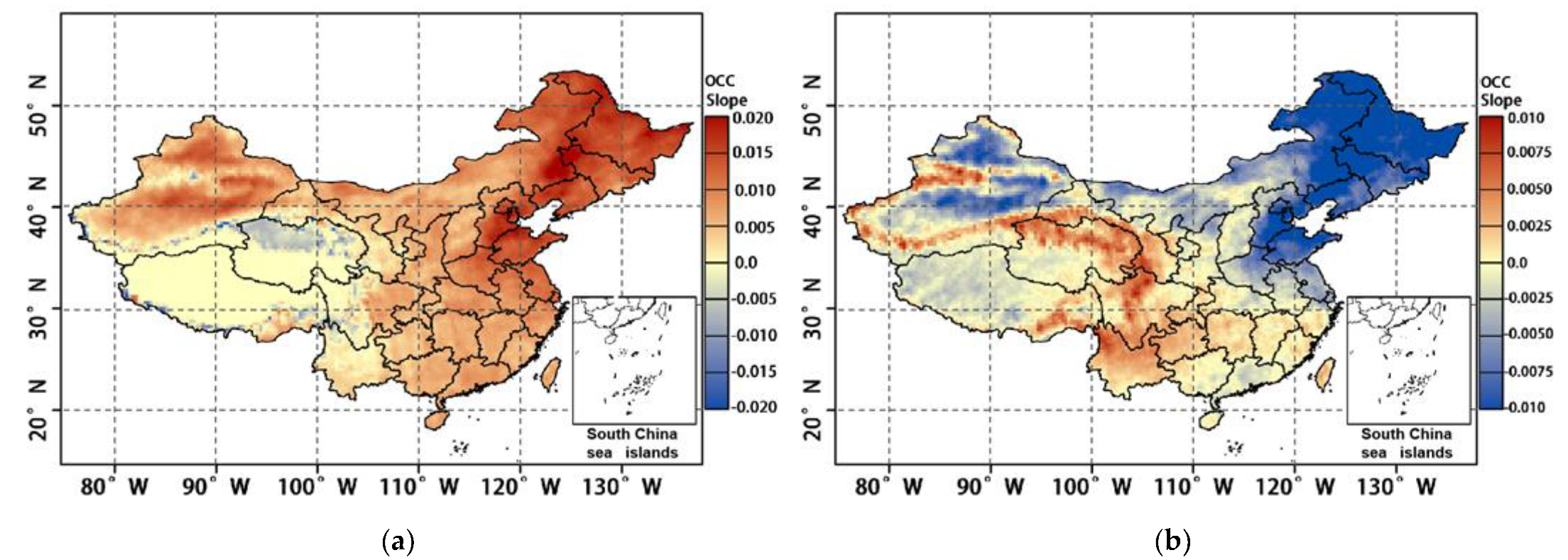
- The vertical distribution characteristics of tropospheric OCC in China from 2005 to 2020 were analysed using OMI ozone profile products. The results show that the OCCLT shows an increasing trend from 2005 to 2020, with a mean year-on-year change of 0.143 DU, and a decreasing trend in the mid-troposphere, with a mean year-on-year change of −0.091 DU; OCC across the troposphere rose by 2.52 DU or 7.9% There is a significant negative correlation between the slopes of the OCCs at the two high layers (with an r of −0.891), which indicates that the OCCLT is affected by the ozone transmission from the mid-troposphere.
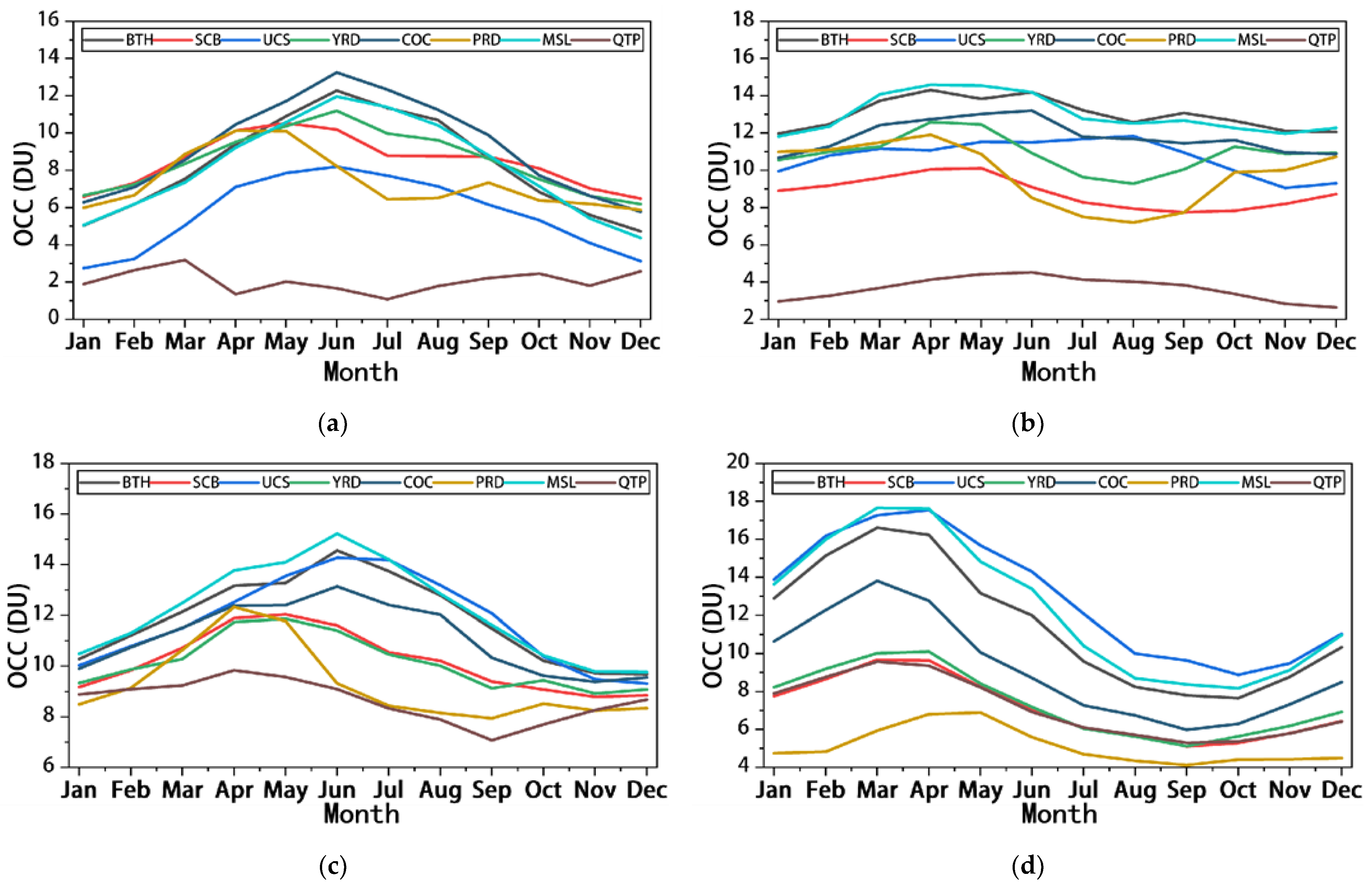
- The variation in OCCs in the different altitudes of the troposphere is characterised by obvious seasonal changes, with the OCCLT being higher in spring (8.22 ± 1.05 DU) and summer (8.80 ± 1.29 DU) than in autumn (6.38 ± 0.77 DU) and winter (5.70 ± 0.48 DU); the extreme values of the OCCLT occur in May or June and peak in the middle troposphere in autumn (9.25 ± 1.19 DU) and winter (10.50 ± 0.45 DU). The mid-troposphere is strongly influenced by topographic conditions; in the upper troposphere it rises continuously in spring (up to 11.84 ± 1.30 DU) and decreases during the rest of the season, while the upper troposphere OCC shows a consistent latitude-dependent trend.
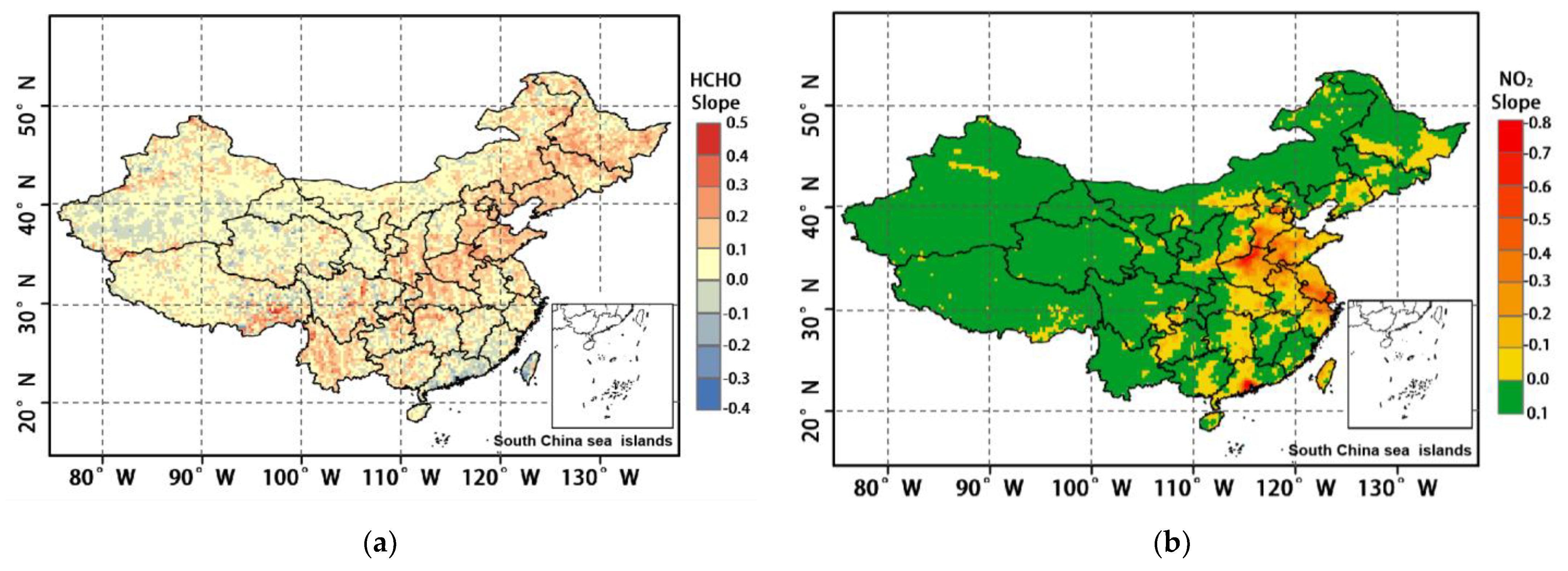
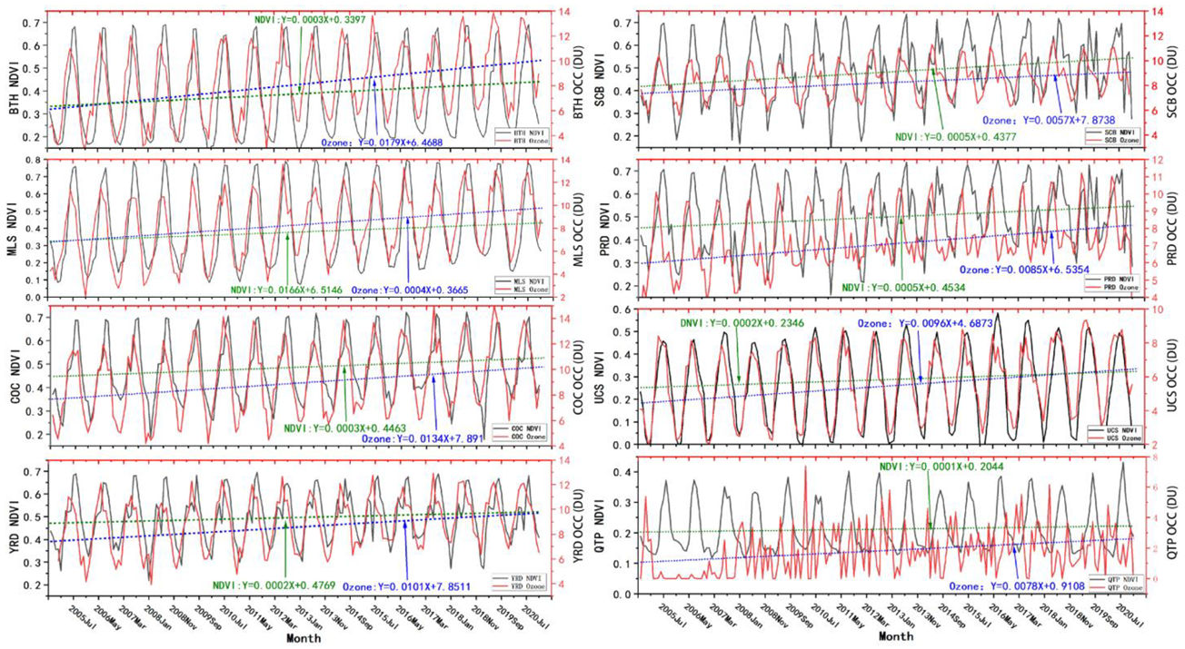
- Analysis based on multi-source data shows that the changes in OCCLT are closely related to ozone precursors, vegetation cover, air temperature, and PBLH. The energy conservation and emission reduction policies in China in recent years have led to a large reduction in NOx, and the increase in VOCs due to natural factors has weakened the titration of ozone production and contributed to the increase in OCCLT. The NDVI shows a fluctuating upward trend, and the vegetation growth shows a positive correlation with the OCCLT, with an r > 0.6 in most regions of China; the temperature of the lower troposphere in China increases significantly (+0.63 °C), which strengthens the photochemical reaction of ozone. In addition, the increase in the PBLH also plays a positive role in the increase in the OCCLT.
Author Contributions
Funding
Institutional Review Board Statement
Informed Consent Statement
Data Availability Statement
Acknowledgments
Conflicts of Interest
Abbreviations
| Abbreviations | Full name |
| BTH | Beijing-Tianjin-Hebei |
| CMA | China meteorological administration |
| COC | centre of China |
| DU | Dobson units |
| MLS | microwave limb sounder |
| MSL | mid-southern Liaoning |
| MYC | mean year-on-year changes |
| NOx | nitrogen oxides |
| OCC | ozone column concentration |
| OCCLT | OCC in the lower troposphere |
| OMI | ozone monitoring instrument |
| PBLH | planetary boundary layer height |
| PRD | Pearl river delta |
| QTP | Qinghai--Tibet plateau |
| SCB | Sichuan basin |
| TOC | total organic carbon |
| UCS | Urumqi-Changji--Shihezi |
| VOCs | volatile organic compounds |
| YRD | Yangtze river delta |
References
- Hollósy, F. Effects of ultraviolet radiation on plant cells. Micron 2002, 33, 179–197. [Google Scholar] [CrossRef]
- Nowack, P.J.; Abraham, N.L.; Braesicke, P.; Pyle, J.A. Stratospheric ozone changes under solar geoengineering: Implications for UV exposure and air quality. Atmos. Chem. Phys. 2016, 16, 4191–4203. [Google Scholar] [CrossRef] [Green Version]
- Bornman, J.F.; Barnes, P.W.; Robson, T.M.; Robinson, S.A.; Jansen, M.A.; Ballare, C.L.; Flint, S.D. Linkages between stratospheric ozone, UV radiation and climate change and their implications for terrestrial ecosystems. Photochem. Photobiol. Sci. 2019, 18, 681–716. [Google Scholar] [CrossRef] [Green Version]
- Guenther, A.; Karl, T.; Harley, P.; Wiedinmyer, C.; Palmer, P.I.; Geron, C. Estimates of global terrestrial isoprene emissions using MEGAN (Model of Emissions of Gases and Aerosols from Nature). Atmos. Chem. Phys. 2006, 6, 3181–3210. [Google Scholar] [CrossRef] [Green Version]
- Burkart, S.; Bender, J.; Tarkotta, B.; Faust, S.; Castagna, A.; Ranieri, A.; Weigel, H.J. Effects of ozone on leaf senescence, photochemical efficiency and grain yield in two winter wheat cultivars. J. Agron. Crop Sci. 2013, 199, 275–285. [Google Scholar] [CrossRef]
- Cohen, A.J.; Brauer, M.; Burnett, R.; Anderson, H.R.; Frostad, J.; Estep, K.; Balakrishnan, K.; Brunekreef, B.; Dandona, L.; Dandona, R. Estimates and 25-year trends of the global burden of disease attributable to ambient air pollution: An analysis of data from the Global Burden of Diseases Study 2015. Lancet 2017, 389, 1907–1918. [Google Scholar] [CrossRef] [Green Version]
- Avnery, S.; Mauzerall, D.L.; Liu, J.; Horowitz, L.W. Global crop yield reductions due to surface ozone exposure: 2. Year 2030 potential crop production losses and economic damage under two scenarios of O3 pollution. Atmos. Environ. 2011, 45, 2297–2309. [Google Scholar] [CrossRef]
- Tang, X.Y.; Li, J.L.; Dong, Z.X. Photochemical Pollution in Lanzhou, China-A Case Study. J. Environ. Sci. 1989, 58, 384–395. [Google Scholar]
- Kok, G.L.; Lind, J.A.; Fang, M. An airborne study of air quality around the Hong Kong territory. J. Geophys. Res. Atmos. 1997, 102, 19043–19057. [Google Scholar] [CrossRef] [Green Version]
- Wang, T.; Poon, C.; Kwok, Y.; Li, Y.S. Characterizing the temporal variability and emission patterns of pollution plumes in the Pearl River Delta of China. Atmos. Environ. 2003, 37, 3539–3550. [Google Scholar] [CrossRef]
- Xu, X.; Lin, W.; Wang, T.; Yan, P.; Tang, J.; Meng, Z.; Wang, Y. Long-term trend of surface ozone at a regional background station in eastern China 1991–2006: Enhanced variability. Atmos. Chem. Phys. 2008, 8, 2595–2607. [Google Scholar] [CrossRef]
- Tang, G.; Li, X.; Wang, Y.; Xin, J.; Ren, X. Surface ozone trend details and interpretations in Beijing, 2001–2006. Atmos. Chem. Phys. 2009, 9, 8813–8823. [Google Scholar] [CrossRef] [Green Version]
- He, H.; Mu, H.; Yang, L. Spatial Variation of Surface Ozone Concentration During the Warm Season and Its Meteorological Driving Factors in China. Environ. Sci. 2021, 42, 4168–4179. [Google Scholar]
- Shao, M.; Zhang, Y.; Zeng, L.; Tang, X.; Zhang, J.; Zhong, L.; Wang, B. Ground-level ozone in the Pearl River Delta and the roles of VOC and NOx in its production. J. Environ. Manag. 2009, 90, 512–518. [Google Scholar] [CrossRef] [PubMed]
- Noreen, A.; Khokhar, M.F.; Zeb, N.; Yasmin, N.; Hakeem, K.R. Spatio-temporal assessment and seasonal variation of tropospheric ozone in Pakistan during the last decade. Environ. Sci. Pollut. Res. 2018, 25, 8441–8454. [Google Scholar] [CrossRef]
- Chen, X.; Zhong, B.; Huang, F.; Wang, X.; Sarkar, S.; Jia, S.; Deng, X.; Chen, D.; Shao, M. The role of natural factors in constraining long-term tropospheric ozone trends over Southern China. Atmos. Environ. 2020, 220, 117060. [Google Scholar] [CrossRef]
- Lia, Y.; Cheng, M.; Guo, Z.; Zhang, X.; Cui, X.; Chen, S. Increase in surface ozone over Beijing-Tianjin-Hebei and the surrounding areas of China inferred from satellite retrievals, 2005–2018. Aerosol Air Qual. Res. 2020, 20, 2170–2184. [Google Scholar] [CrossRef] [Green Version]
- Hung, R.; Liu, J. Satellite remote sensing and ozonesonde observation of ozone vertical profile and severe storm development. Int. J. Remote Sens. 1988, 9, 469–475. [Google Scholar] [CrossRef]
- Zhao, Z.; Zhou, Z.; Russo, A.; Du, H.; Xiang, J.; Zhang, J.; Zhou, C. Impact of meteorological conditions at multiple scales on ozone concentration in the Yangtze River Delta. Environ. Sci. Pollut. Res. 2021, 28, 62991–63007. [Google Scholar] [CrossRef]
- Junping, D.; Yuxia, Z.; Rui, L.; Tao, X.; Xin, Y. Analysis on Spatiotemporal Characteristics of Total Column Ozone over China Based on OMI Product. Environ. Monit. China 2014, 30, 191–196. [Google Scholar] [CrossRef]
- Zhu, L.; Liu, M.; Song, J. Spatiotemporal Variations and Influent Factors of Tropospheric Ozone Concentration over China Based on OMI Data. Atmosphere 2022, 13, 253. [Google Scholar] [CrossRef]
- Levelt, P.F.; Van Den Oord, G.H.; Dobber, M.R.; Malkki, A.; Visser, H.; De Vries, J.; Stammes, P.; Lundell, J.O.; Saari, H. The ozone monitoring instrument. IEEE Trans. Geosci. Remote Sens. 2006, 44, 1093–1101. [Google Scholar] [CrossRef]
- Heue, K.-P.; Coldewey-Egbers, M.; Delcloo, A.; Lerot, C.; Loyola, D.; Valks, P.; Van Roozendael, M. Trends of tropical tropospheric ozone from 20 years of European satellite measurements and perspectives for the Sentinel-5 Precursor. Atmos. Meas. Tech. 2016, 9, 5037–5051. [Google Scholar] [CrossRef] [Green Version]
- Shen, L.; Jacob, D.J.; Liu, X.; Huang, G.; Li, K.; Liao, H.; Wang, T. An evaluation of the ability of the Ozone Monitoring Instrument (OMI) to observe boundary layer ozone pollution across China: Application to 2005–2017 ozone trends. Atmos. Chem. Phys. 2019, 19, 6551–6560. [Google Scholar] [CrossRef] [Green Version]
- Tianbao, Z.; Ail, L.K.; Jinming, F. An Intercomparison between NCEP Reanalysisand Observed Data over China. Clim. Environ. Res. 2004, 9, 278–294. [Google Scholar]
- Zhao, Q.; Liu, Y.; Guan, Z.; Lu, c.; Cai, z. Anomalous feature of ozone in upper troposphere/lower stratosphere over Beijing in winter 2008. Trans. Atmos. Sci. 2015, 38, 796–803. [Google Scholar]
- Akimoto, H. Global air quality and pollution. Science 2003, 302, 1716–1719. [Google Scholar] [CrossRef] [Green Version]
- Atkinson, R. Gas-phase tropospheric chemistry of volatile organic compounds. J. Phys. Chem. Ref. Data Monog 1994, 2, 11–216. [Google Scholar]
- Zhu, L.; Jacob, D.J.; Keutsch, F.N.; Mickley, L.J.; Scheffe, R.; Strum, M.; González Abad, G.; Chance, K.; Yang, K.; Rappenglück, B.; et al. Formaldehyde (HCHO) as a hazardous air pollutant: Mapping surface air concentrations from satellite and inferring cancer risks in the United States. Environ. Sci. Technol. 2017, 51, 5650–5657. [Google Scholar] [CrossRef]
- Li, R.; Xu, M.; Li, M.; Chen, Z.; Zhao, N.; Gao, B.; Yao, Q. Identifying the spatiotemporal variations in ozone formation regimes across China from 2005 to 2019 based on polynomial simulation and causality analysis. Atmos. Chem. Phys. 2021, 21, 15631–15646. [Google Scholar] [CrossRef]
- Ma, M.; Yao, G.; Guo, J.; Bai, K. Distinct spatiotemporal variation patterns of surface ozone in China due to diverse influential factors. J. Environ. Manag. 2021, 288, 112368. [Google Scholar] [CrossRef] [PubMed]
- Ren, Y.; Qu, Z.; Du, Y.; Xu, R.; Ma, D.; Yang, G.; Shi, Y.; Fan, X.; Tani, A.; Guo, P. Air quality and health effects of biogenic volatile organic compounds emissions from urban green spaces and the mitigation strategies. Environ. Pollut. 2017, 230, 849–861. [Google Scholar] [CrossRef] [PubMed]
- Wang, Y.; Zhao, Y.; Zhang, L.; Zhang, J.; Liu, Y. Modified regional biogenic VOC emissions with actual ozone stress and integrated land cover information: A case study in Yangtze River Delta, China. Sci. Total Environ. 2020, 727, 138703. [Google Scholar] [CrossRef]
- Fortuin, J.P.; Langematz, U. Update on the global ozone climatology and on concurrent ozone and temperature trends. In Atmospheric Sensing and Modelling; SPIE: Bellingham, DC, USA, 1995; pp. 207–216. [Google Scholar]
- Bloomer, B.J.; Stehr, J.W.; Piety, C.A.; Salawitch, R.J.; Dickerson, R.R. Observed relationships of ozone air pollution with temperature and emissions. Geophys. Res. Lett. 2009, 36, L09803. [Google Scholar] [CrossRef] [Green Version]
- Chen, Z.; Li, R.; Chen, D.; Zhuang, Y.; Gao, B.; Yang, L.; Li, M. Understanding the causal influence of major meteorological factors on ground ozone concentrations across China. J. Clean. Prod. 2020, 242, 118498. [Google Scholar] [CrossRef]
- Solomon, S.; Qin, D.; Manning, M.; Chen, Z.; Marquis, M.; Averyt, K.B.; Tignor, M.; Miller, H.L. IPCC Summary for Policymakers. In Climate Change 2007: The Physical Science Basis. Contribution of Working Group I to the Fourth Assessment Report of the Intergovernmental Panel on Climate Change; Cambridge University Press: Cambridge, UK, 2007; pp. 1–18. [Google Scholar]
- Yan, R.; Chen, M.; Gao, Q.; Liu, T.; Hu, S.; Gao, W. Characteristics of typical ozone pollution distribution and impact factors in Beijing in summer. Res. Environ. Sci. 2013, 26, 43–49. [Google Scholar]
- Tang, G.; Liu, Y.; Huang, X.; Wang, Y.; Hu, B.; Zhang, Y.; Song, T.; Li, X.; Wu, S.; Li, Q. Aggravated ozone pollution in the strong free convection boundary layer. Sci. Total Environ. 2021, 788, 147740. [Google Scholar] [CrossRef]
- Karle, N.N.; Fitzgerald, R.M.; Sakai, R.K.; Sullivan, D.W.; Stockwell, W.R. Multi-Scale Atmospheric Emissions, Circulation and Meteorological Drivers of Ozone Episodes in El Paso-Juárez Airshed. Atmosphere 2021, 12, 1575. [Google Scholar] [CrossRef]
- Karle, N.N.; Mahmud, S.; Sakai, R.K.; Fitzgerald, R.M.; Morris, V.R.; Stockwell, W.R. Investigation of the successive ozone episodes in the El Paso–Juarez region in the summer of 2017. Atmosphere 2020, 11, 532. [Google Scholar] [CrossRef]
- Hallar, A.G.; Brown, S.S.; Crosman, E.; Barsanti, K.C.; Cappa, C.D.; Faloona, I.; Fast, J.; Holmes, H.A.; Horel, J.; Lin, J. Coupled Air Quality and Boundary-Layer Meteorology in Western US Basins during Winter: Design and Rationale for a Comprehensive Study. Bull. Am. Meteorol. Soc. 2021, 102, E2012–E2033. [Google Scholar] [CrossRef]
- Jin, X.; Fiore, A.; Boersma, K.F.; Smedt, I.D.; Valin, L. Inferring changes in summertime surface Ozone–NO x–VOC chemistry over US urban areas from two decades of satellite and ground-based observations. Environ. Sci. Technol. 2020, 54, 6518–6529. [Google Scholar] [CrossRef] [PubMed]
- Lee, H.-J.; Chang, L.-S.; Jaffe, D.A.; Bak, J.; Liu, X.; Abad, G.G.; Jo, H.-Y.; Jo, Y.-J.; Lee, J.-B.; Yang, G.-H. Satellite-Based Diagnosis and Numerical Verification of Ozone Formation Regimes over Nine Megacities in East Asia. Remote Sens. 2022, 14, 1285. [Google Scholar] [CrossRef]
- Jin, X.; Holloway, T. Spatial and temporal variability of ozone sensitivity over China observed from the Ozone Monitoring Instrument. J. Geophys. Res. Atmos. 2015, 120, 7229–7246. [Google Scholar] [CrossRef]
- Lee, H.-J.; Chang, L.-S.; Jaffe, D.A.; Bak, J.; Liu, X.; Abad, G.G.; Jo, H.-Y.; Jo, Y.-J.; Lee, J.-B.; Kim, C.-H. Ozone continues to increase in East Asia despite decreasing NO2: Causes and abatements. Remote Sens. 2021, 13, 2177. [Google Scholar] [CrossRef]
- Wang, N.; Lyu, X.; Deng, X.; Huang, X.; Jiang, F.; Ding, A. Aggravating O3 pollution due to NOx emission control in eastern China. Sci. Total Environ. 2019, 677, 732–744. [Google Scholar] [CrossRef]
- Barkley, M.P.; Smedt, I.D.; Van Roozendael, M.; Kurosu, T.P.; Chance, K.; Arneth, A.; Hagberg, D.; Guenther, A.; Paulot, F.; Marais, E. Top-down isoprene emissions over tropical South America inferred from SCIAMACHY and OMI formaldehyde columns. J. Geophys. Res. Atmos. 2013, 118, 6849–6868. [Google Scholar] [CrossRef]
- Alves, E.G.; Harley, P.; Gonçalves, J.F.d.C.; Moura, C.E.d.S.; Jardine, K. Effects of light and temperature on isoprene emission at different leaf developmental stages of Eschweilera coriacea in central Amazon. Acta Amaz. 2014, 44, 9–18. [Google Scholar] [CrossRef]
- Tie, X.; Li, G.; Ying, Z.; Guenther, A.; Madronich, S. Biogenic emissions of isoprenoids and NO in China and comparison to anthropogenic emissions. Sci. Total Environ. 2006, 371, 238–251. [Google Scholar] [CrossRef] [Green Version]
- Nemecek-Marshall, M.; MacDonald, R.C.; Franzen, J.J.; Wojciechowski, C.L.; Fall, R. Methanol Emission from Leaves (Enzymatic Detection of Gas-Phase Methanol and Relation of Methanol Fluxes to Stomatal Conductance and Leaf Development). Plant Physiol. 1995, 108, 1359–1368. [Google Scholar] [CrossRef] [Green Version]
- Liu, Y.; Li, L.; An, J.; Huang, L.; Yan, R.; Huang, C.; Wang, H.; Wang, Q.; Wang, M.; Zhang, W. Estimation of biogenic VOC emissions and its impact on ozone formation over the Yangtze River Delta region, China. Atmos. Environ. 2018, 186, 113–128. [Google Scholar] [CrossRef]


| Urban Agglomerations | Spatial Range |
|---|---|
| Beijing-Tianjin-Hebei | 114–119.5° E, 37–42° N |
| Yangtze River Delta | 116.5–122° E, 27.5–34° N |
| Urumqi-Changji-Shihezi | 86.5–89° E, 42.5–45° N |
| Qinghai-Tibet Plateau | 73–105° E, 36–40° N |
| Pearl River Delta | 111–115° E, 22–25° N |
| Sichuan Basin | 103.5–109° E, 28.5–32° N |
| Centre of China | 111–116° E, 32–37° N |
| Mid-Southern Liaoning | 121–125° E, 38.5–42.5° N |
| High Level | Altitude (km) | Atmospheric Pressure (hPa) |
|---|---|---|
| Layer-15 | 9.6–12.8 | 300 |
| Layer-16 | 5.8–9.6 | 500 |
| Layer-17 | 3–5.8 | 700 |
| Layer-18 | 0–3 | 1000 |
| Area | 0–3 km | 3–5.8 km | 5.8–9.6 km | 9.6–12.4 km |
|---|---|---|---|---|
| BTH | 0.239 | −0.200 | −0.014 | −0.034 |
| SCB | 0.074 | −0.011 | 0.032 | 0.009 |
| UCS | 0.132 | −0.063 | −0.012 | −0.022 |
| YRD | 0.155 | −0.091 | 0.001 | −0.008 |
| COC | 0.166 | −0.113 | −0.015 | −0.013 |
| PRD | 0.105 | −0.061 | 0.005 | −0.002 |
| MSL | 0.205 | −0.163 | −0.007 | −0.035 |
| QTP | 0.064 | −0.019 | 0.053 | −0.007 |
| Mean | 0.143 | −0.091 | 0.005 | −0.014 |
| Altitude Layer (km) | Number of Samples | Correlation Coefficient |
|---|---|---|
| 53.3–57 | 10,766 | 0.264 |
| 48–53.3 | 0.334 | |
| 42.8–48 | 0.497 | |
| 40–42.8 | 0.457 | |
| 36–40 | 0.319 | |
| 33.7–36 | 0.374 | |
| 31.4–33.7 | 0.494 | |
| 26.7–31.4 | 0.429 | |
| 24–26.7 | −0.283 | |
| 21–24 | −0.261 | |
| 18.8–24 | −0.001 | |
| 16.7–18.8 | 0.583 | |
| 14.3–16.7 | 0.787 | |
| 12.4–14.3 | 0.789 | |
| 9.6–12.4 | 0.805 | |
| 5.8–9.6 | 0.284 | |
| 0–3 | 9290 | −0.891 |
| Area | r | Fitted Formula |
|---|---|---|
| UCS | 0.875 | y = 26.0044x + 3.05747 |
| MSL | 0.793 | y = 16.115x + 4.23403 |
| COC | 0.785 | y = 16.115x + 4.23403 |
| BTH | 0.746 | y = 18.2164x + 4.18514 |
| YRD | 0.630 | y = 16.9844x + 4.32518 |
| SCB | 0.613 | y = 9.44341x + 5.86769 |
| PRD | 0.330 | y = 4.39351x + 6.11428 |
| QTP | −0.184 | y = −6.23702x + 2.90587 |
Publisher’s Note: MDPI stays neutral with regard to jurisdictional claims in published maps and institutional affiliations. |
© 2022 by the authors. Licensee MDPI, Basel, Switzerland. This article is an open access article distributed under the terms and conditions of the Creative Commons Attribution (CC BY) license (https://creativecommons.org/licenses/by/4.0/).
Share and Cite
Zhang, Y.; Zhang, Y.; Liu, Z.; Bi, S.; Zheng, Y. Analysis of Vertical Distribution Changes and Influencing Factors of Tropospheric Ozone in China from 2005 to 2020 Based on Multi-Source Data. Int. J. Environ. Res. Public Health 2022, 19, 12653. https://doi.org/10.3390/ijerph191912653
Zhang Y, Zhang Y, Liu Z, Bi S, Zheng Y. Analysis of Vertical Distribution Changes and Influencing Factors of Tropospheric Ozone in China from 2005 to 2020 Based on Multi-Source Data. International Journal of Environmental Research and Public Health. 2022; 19(19):12653. https://doi.org/10.3390/ijerph191912653
Chicago/Turabian StyleZhang, Yong, Yang Zhang, Zhihong Liu, Sijia Bi, and Yuni Zheng. 2022. "Analysis of Vertical Distribution Changes and Influencing Factors of Tropospheric Ozone in China from 2005 to 2020 Based on Multi-Source Data" International Journal of Environmental Research and Public Health 19, no. 19: 12653. https://doi.org/10.3390/ijerph191912653
APA StyleZhang, Y., Zhang, Y., Liu, Z., Bi, S., & Zheng, Y. (2022). Analysis of Vertical Distribution Changes and Influencing Factors of Tropospheric Ozone in China from 2005 to 2020 Based on Multi-Source Data. International Journal of Environmental Research and Public Health, 19(19), 12653. https://doi.org/10.3390/ijerph191912653