
Beyond a Spray: Pesticide Application Management in Rural China Based on Quadrilateral Evolutionary Game
Abstract
:1. Introduction
2. Materials and Methods
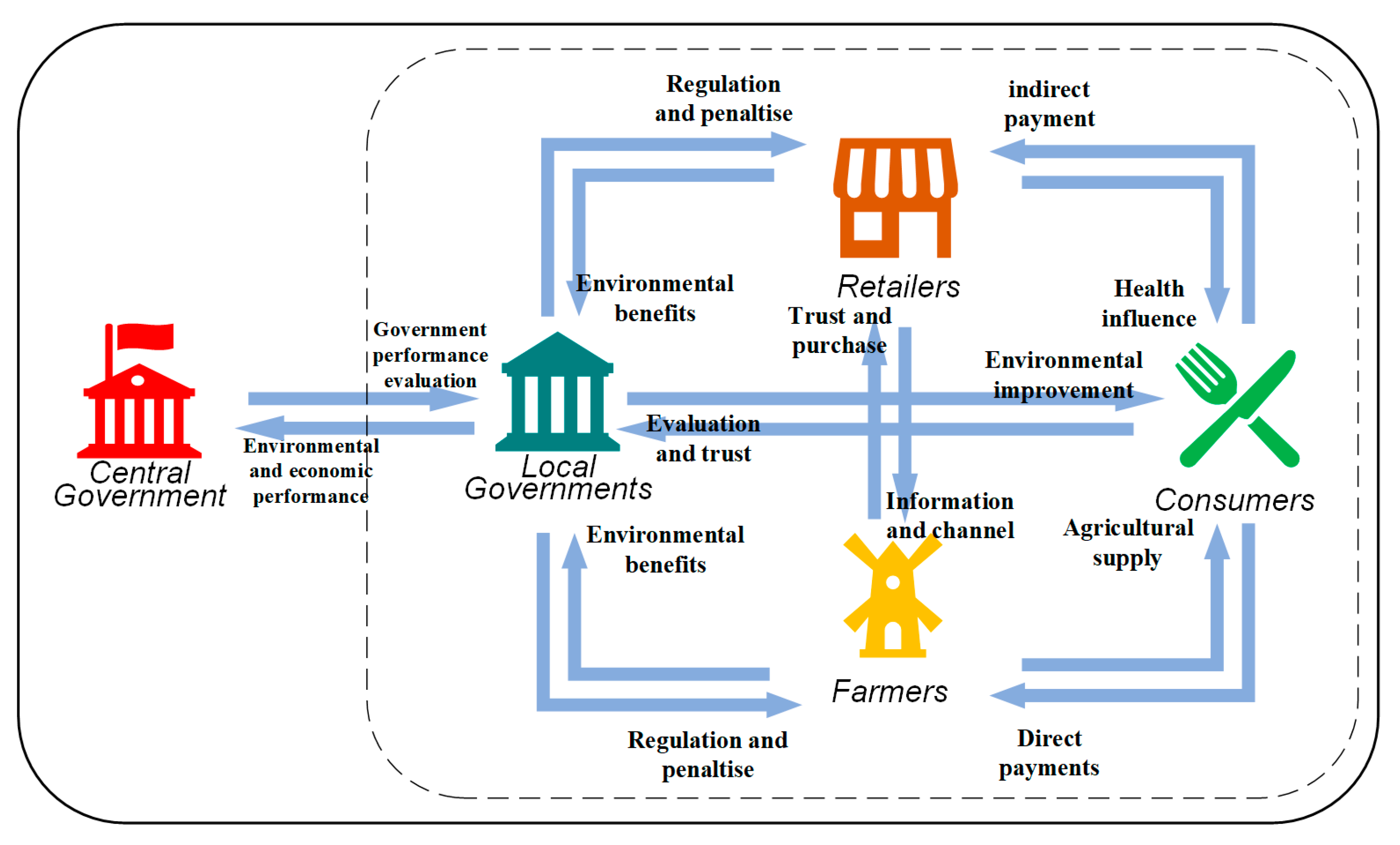
2.1. Stakeholders and Game Framework
2.2. Game Model Assumptions
2.2.1. Assumption 1
2.2.2. Assumption 2
2.2.3. Assumption 3
2.2.4. Assumption 4
2.3. Game Model Establishment
2.4. Equilibrium Solution of the Quadrilateral Evolutionary Game
2.4.1. Stability Analysis of Equilibrium Points When Local Governments Choose Loose Regulation ()
2.4.2. Stability Analysis of Equilibrium Points When Local Governments Choose Strict Regulation ()
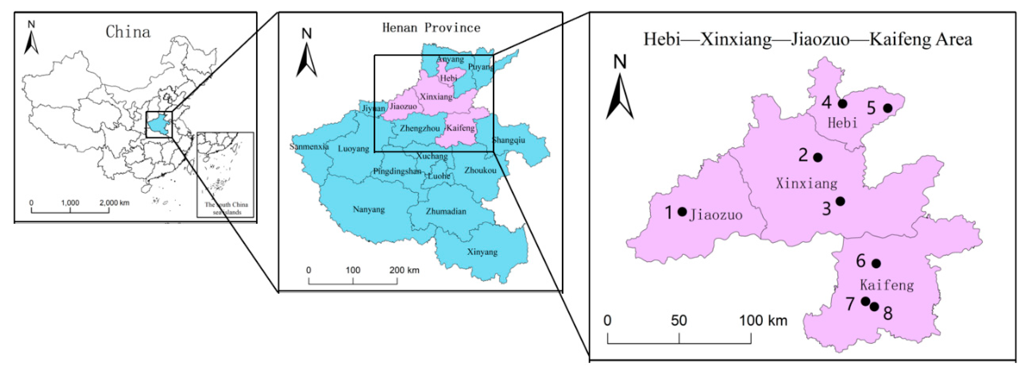
2.5. Data Sources
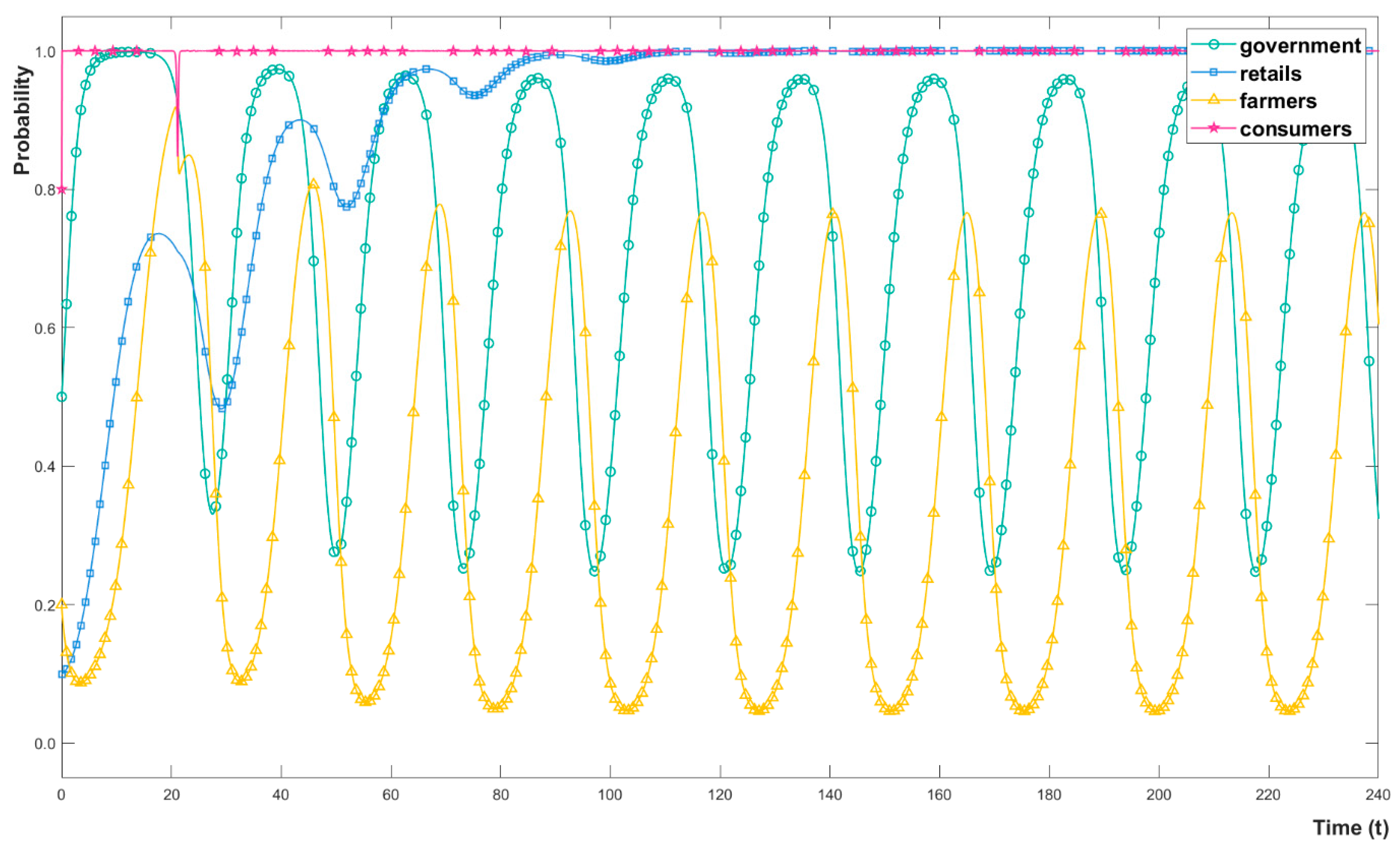
3. Result
4. Discussion
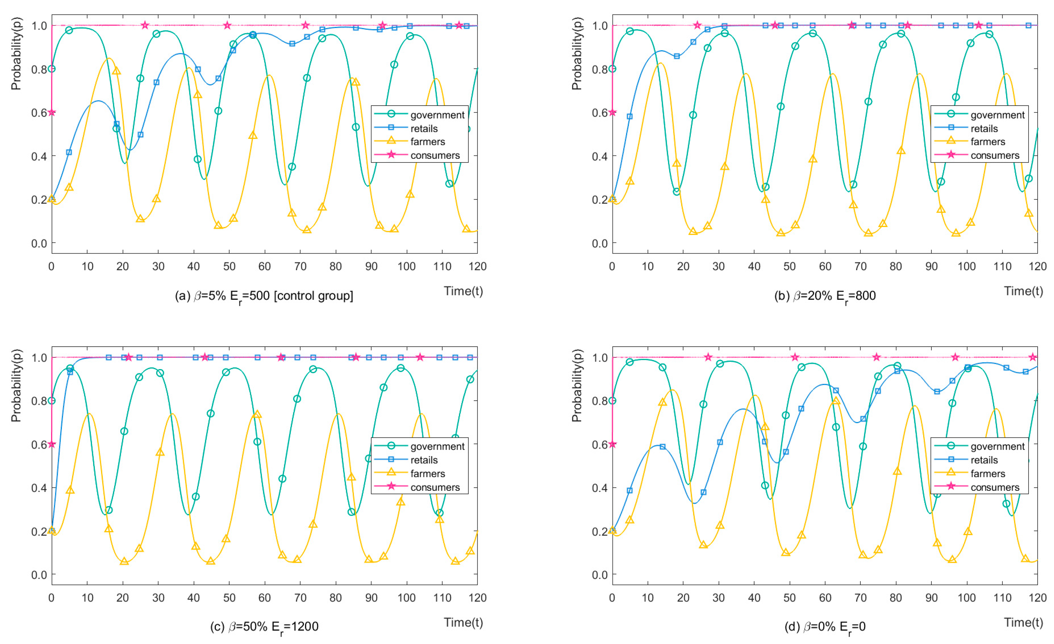
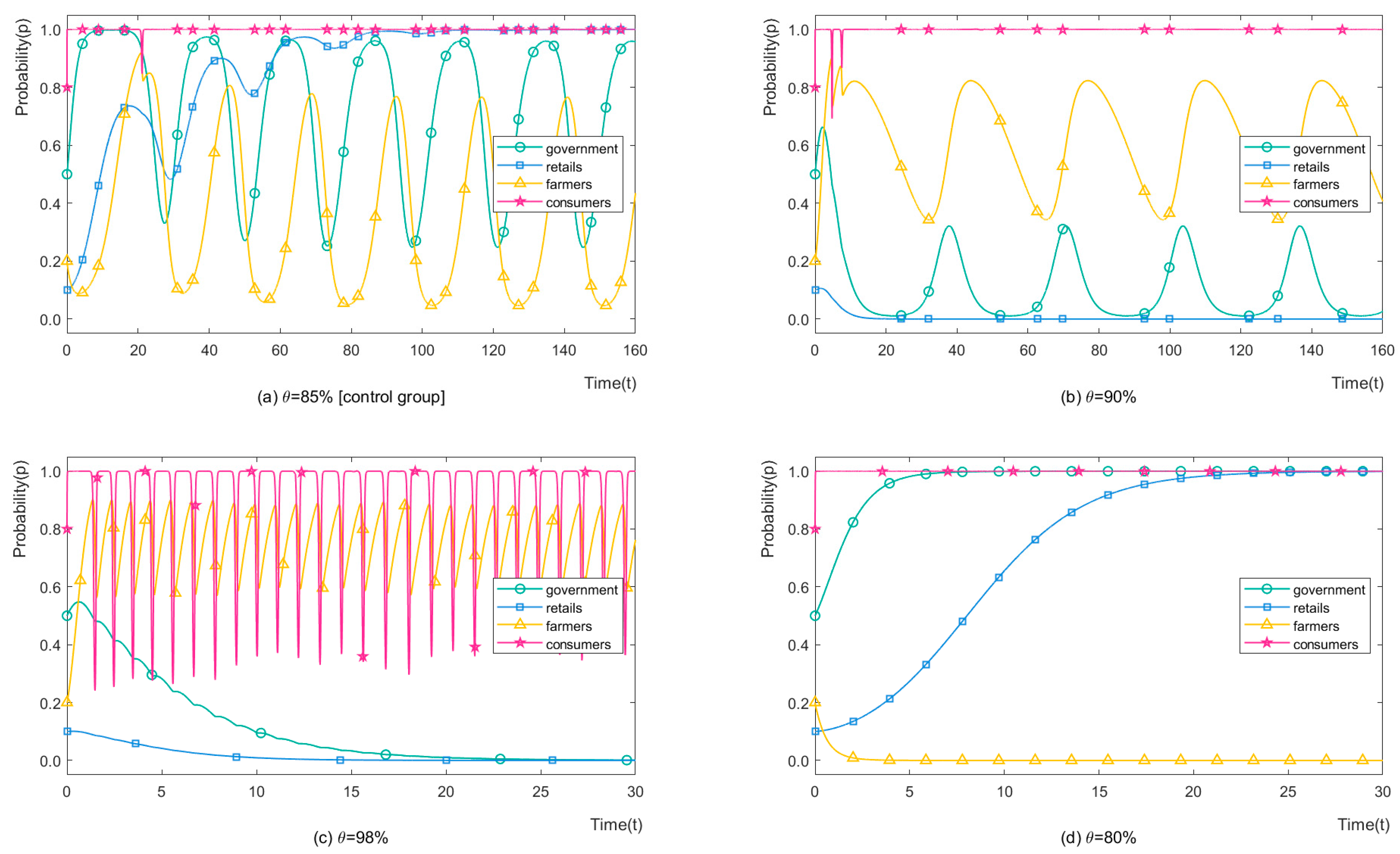
4.1. The Probability () and Economic Loss () of Retailers
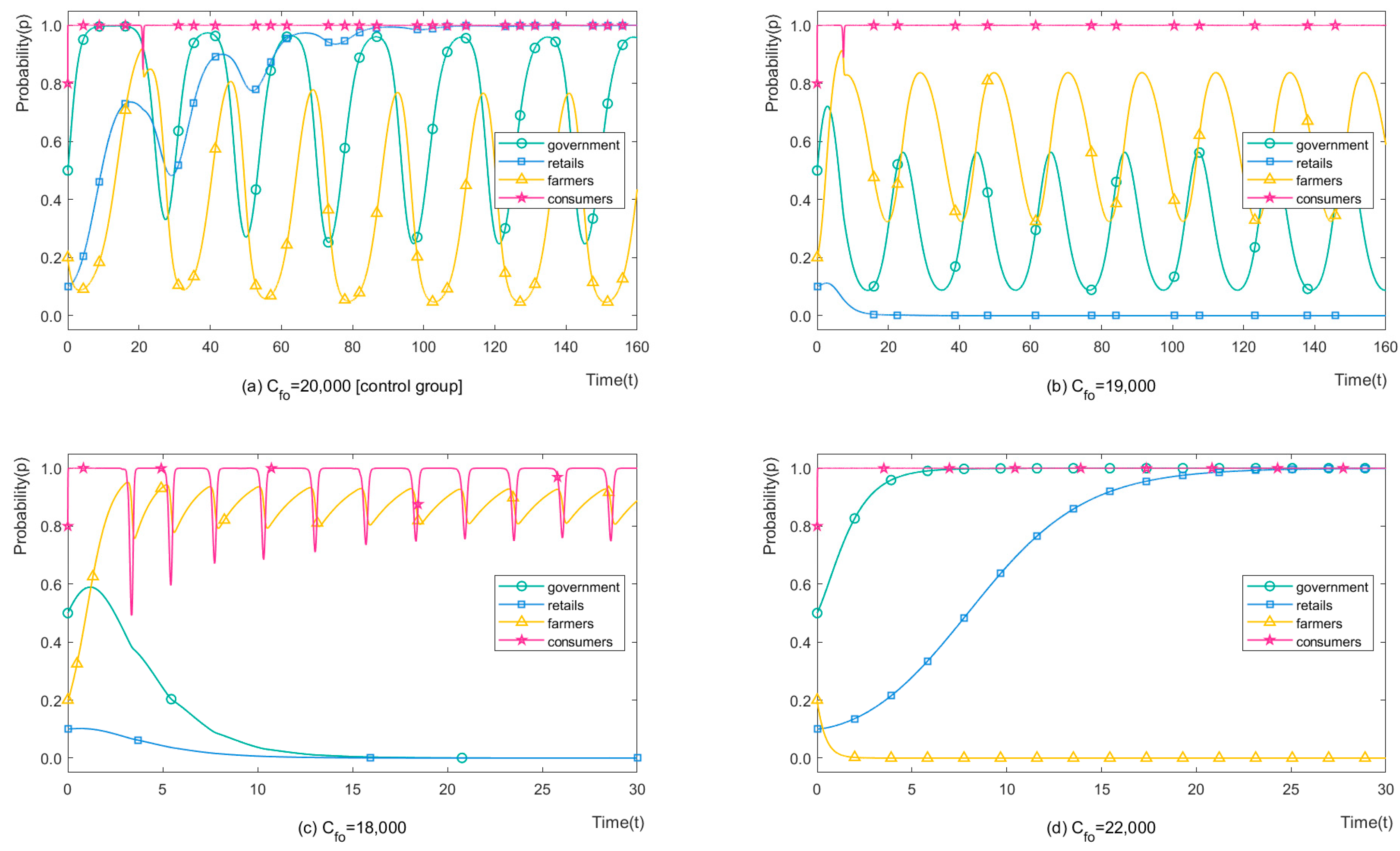
4.2. The Organic Certification Cost () for Farmers
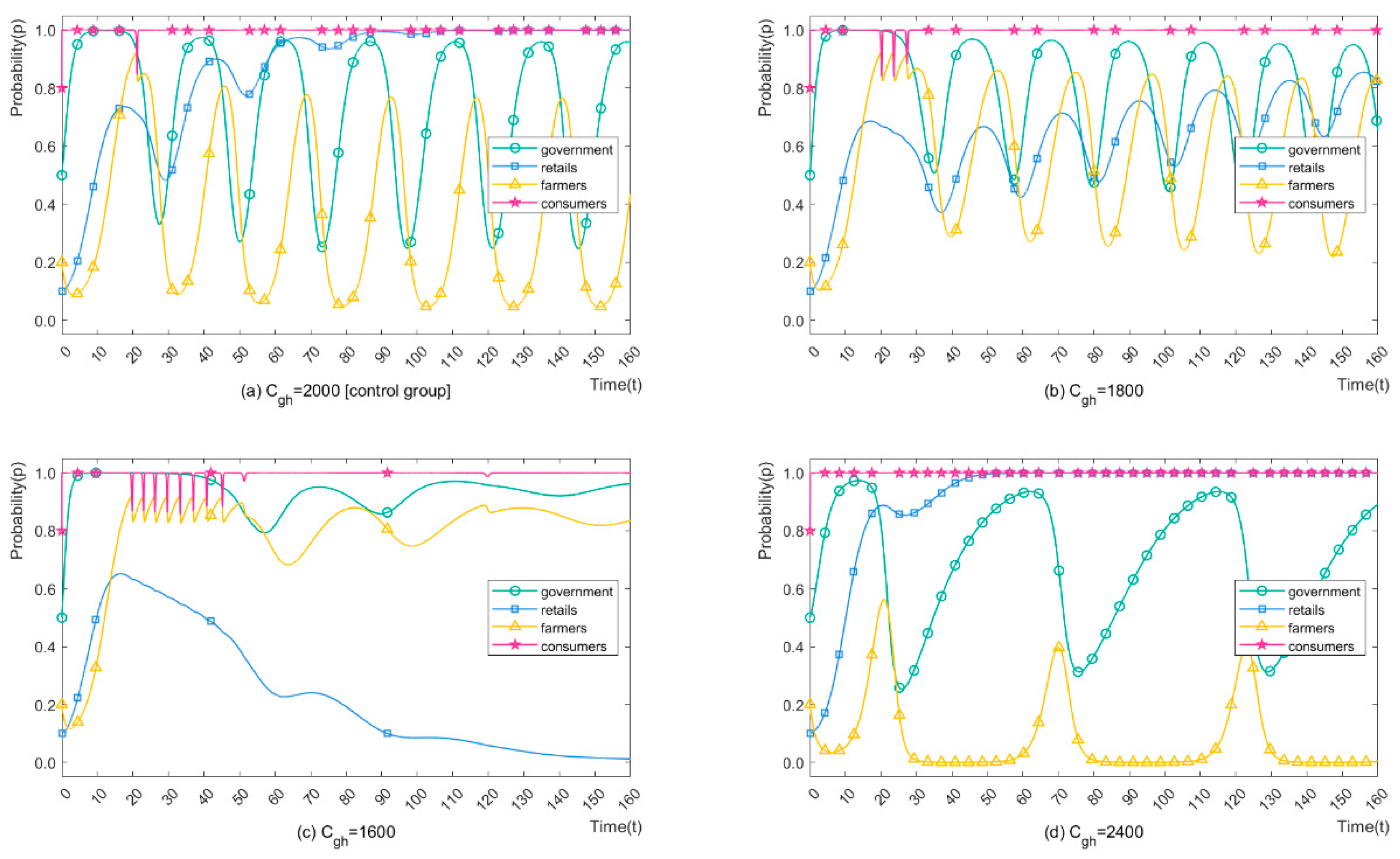
4.3. The Strict Regulation Cost () of Local Governments
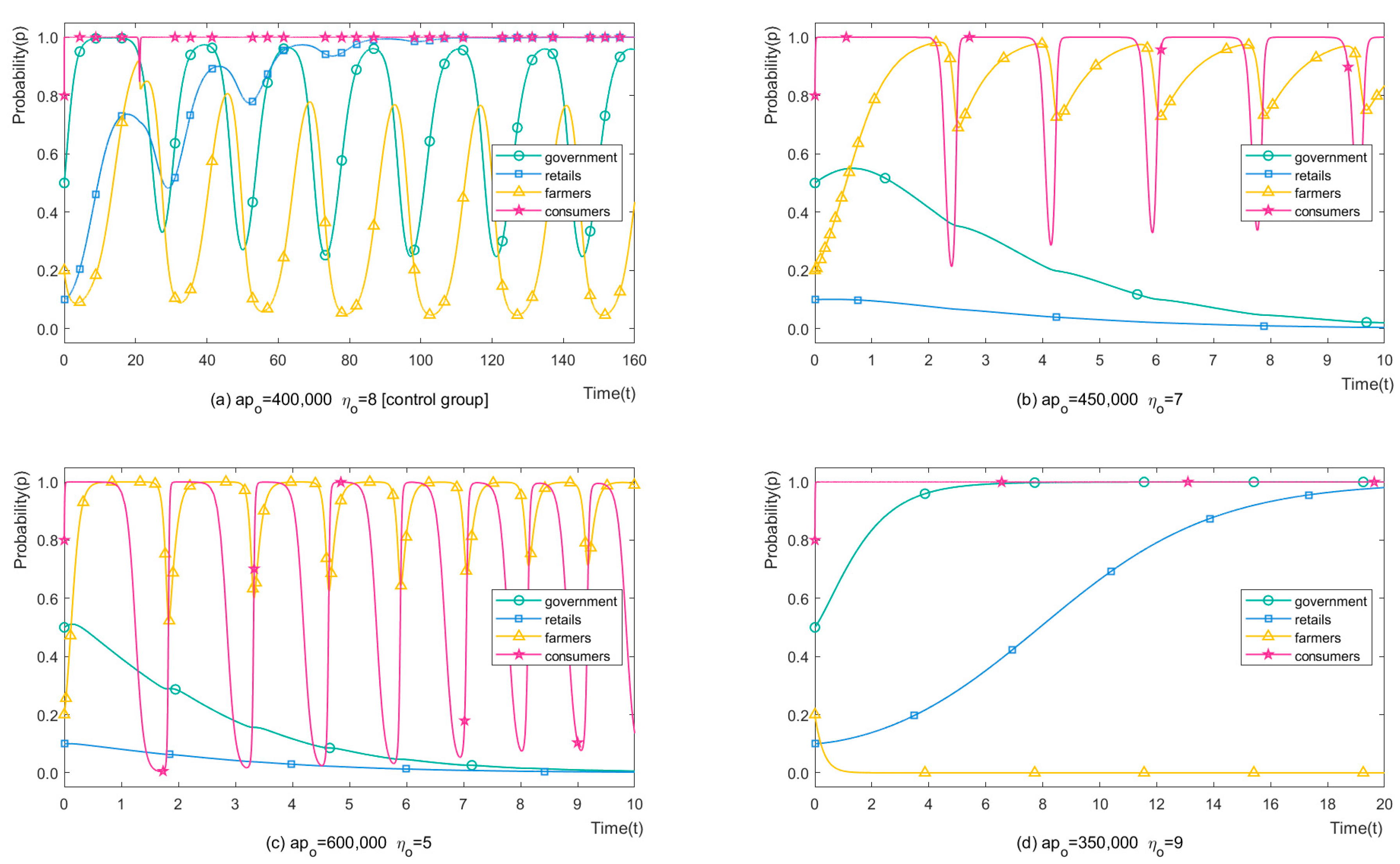
4.4. The Purchase Price of OAPs () and Premium ()
5. Conclusions
Author Contributions
Funding
Institutional Review Board Statement
Informed Consent Statement
Data Availability Statement
Conflicts of Interest
Appendix A. Calculative Process in Section 2.3
Appendix B. Calculative Process in Section 2.4
References
- Zhao, X.; Cui, H.; Wang, Y.; Sun, C.; Cui, B.; Zeng, Z. Development Strategies and Prospects of Nano-based Smart Pesticide Formulation. J. Agric. Food Chem. 2018, 66, 6504–6512. [Google Scholar] [CrossRef]
- Riedo, J.; Wettstein, F.E.; Rosch, A.; Herzog, C.; Banerjee, S.; Buchi, L.; Charles, R.; Wachter, D.; Martin-Laurent, F.; Bucheli, T.D.; et al. Widespread Occurrence of Pesticides in Organically Managed Agricultural Soils-the Ghost of a Conventional Agricultural Past? Environ. Sci. Technol. 2021, 55, 2919–2928. [Google Scholar] [CrossRef] [PubMed]
- Bexfield, L.M.; Belitz, K.; Lindsey, B.D.; Toccalino, P.L.; Nowell, L.H. Pesticides and Pesticide Degradates in Groundwater Used for Public Supply across the United States: Occurrence and Human-Health Context. Environ. Sci. Technol. 2021, 55, 362–372. [Google Scholar] [CrossRef] [PubMed]
- Henry, M.; Beguin, M.; Requier, F.; Rollin, O.; Odoux, J.-F.; Aupinel, P.; Aptel, J.; Tchamitchian, S.; Decourtye, A. A Common Pesticide Decreases Foraging Success and Survival in Honey Bees. Science 2012, 336, 348–350. [Google Scholar] [CrossRef] [PubMed]
- Pelosi, C.; Barot, S.; Capowiez, Y.; Hedde, M.; Vandenbulcke, F. Pesticides and earthworms. A review. Agron. Sustain. Dev. 2014, 34, 199–228. [Google Scholar] [CrossRef]
- Guedes, R.N.C.; Smagghe, G.; Stark, J.D.; Desneux, N. Pesticide-Induced Stress in Arthropod Pests for Optimized Integrated Pest Management Programs. Annu. Rev. Entomol. 2016, 61, 43–62. [Google Scholar] [CrossRef]
- Fenner, K.; Canonica, S.; Wackett, L.P.; Elsner, M. Evaluating Pesticide Degradation in the Environment: Blind Spots and Emerging Opportunities. Science 2013, 341, 752–758. [Google Scholar] [CrossRef]
- Gould, F.; Brown, Z.S.; Kuzma, J. Wicked evolution: Can we address the sociobiological dilemma of pesticide resistance? Science 2018, 360, 728–732. [Google Scholar] [CrossRef]
- Hernandez, A.F.; Parron, T.; Tsatsakis, A.M.; Requena, M.; Alarcon, R.; Lopez-Guarnido, O. Toxic effects of pesticide mixtures at a molecular level: Their relevance to human health. Toxicology 2013, 307, 136–145. [Google Scholar] [CrossRef]
- Mostafalou, S.; Abdollahi, M. Pesticides: An update of human exposure and toxicity. Arch. Toxicol. 2017, 91, 549–599. [Google Scholar] [CrossRef]
- Pretty, J.; Bharucha, Z.P. Integrated Pest Management for Sustainable Intensification of Agriculture in Asia and Africa. Insects 2015, 6, 152–182. [Google Scholar] [CrossRef]
- Singh, A.; Dhiman, N.; Kar, A.K.; Singh, D.; Purohit, M.P.; Ghosh, D.; Patriaik, S. Advances in controlled release pesticide formulations: Prospects to safer integrated pest management and sustainable agriculture. J. Hazard. Mater. 2020, 385, 121525. [Google Scholar] [CrossRef] [PubMed]
- Umetsu, N.; Shirai, Y. Development of novel pesticides in the 21st century. J. Pestic. Sci. 2020, 45, 54–74. [Google Scholar] [CrossRef] [PubMed]
- Stadlinger, N.; Mmochi, A.J.; Kumblad, L. Weak Governmental Institutions Impair the Management of Pesticide Import and Sales in Zanzibar. Ambio 2013, 42, 72–82. [Google Scholar] [CrossRef]
- Wang, Y.; Wang, Y.; Huo, X.; Zhu, Y. Why some restricted pesticides are still chosen by some farmers in China? Empirical evidence from a survey of vegetable and apple growers. Food Control 2015, 51, 417–424. [Google Scholar] [CrossRef]
- Cantrell, C.L.; Dayan, F.E.; Duke, S.O. Natural Products as Sources for New Pesticides. J. Nat. Prod. 2012, 75, 1231–1242. [Google Scholar] [CrossRef] [PubMed]
- Zhan, X.; Shao, C.; He, R.; Shi, R. Evolution and Efficiency Assessment of Pesticide and Fertiliser Inputs to Cultivated Land in China. Int. J. Environ. Res. Public Health 2021, 18, 3771. [Google Scholar] [CrossRef]
- Jin, S.; Bluemling, B.; Mol, A.P.J. Information, trust and pesticide overuse: Interactions between retailers and cotton farmers in China. NJAS Wagening. J. Life Sci. 2015, 72–73, 23–32. [Google Scholar] [CrossRef]
- Chen, Z.-l.; Dong, F.-s.; Xu, J.; Liu, X.-g.; Zheng, Y.-q. Management of pesticide residues in China. J. Integr. Agric. 2015, 14, 2319–2327. [Google Scholar] [CrossRef]
- Sun, S.; Hu, R.; Zhang, C.; Shi, G. Do farmers misuse pesticides in crop production in China? Evidence from a farm household survey. Pest Manag. Sci. 2019, 75, 2133–2141. [Google Scholar] [CrossRef]
- Xu, X.; Li, L.; Huang, X.; Lin, H.; Liu, G.; Xu, D.; Jiang, J. Survey of Four Groups of Cumulative Pesticide Residues in 12 Vegetables in 15 Provinces in China. J. Food Prot. 2018, 81, 377–385. [Google Scholar] [CrossRef] [PubMed]
- Zhao, L.; Wang, C.; Gu, H.; Yue, C. Market incentive, government regulation and the behavior of pesticide application of vegetable farmers in China. Food Control 2018, 85, 308–317. [Google Scholar] [CrossRef]
- Zhou, J.; Jin, S. Safety of vegetables and the use of pesticides by farmers in China: Evidence from Zhejiang province. Food Control 2009, 20, 1043–1048. [Google Scholar] [CrossRef]
- Zhang, H.; Lu, Y. End-users’ knowledge, attitude, and behavior towards safe use of pesticides: A case study in the Guanting Reservoir area, China. Environ. Geochem. Health 2007, 29, 513–520. [Google Scholar] [CrossRef] [PubMed]
- Gong, Y.; Baylis, K.; Kozak, R.; Bull, G. Farmers’ risk preferences and pesticide use decisions: Evidence from field experiments in China. Agric. Econ. 2016, 47, 411–421. [Google Scholar] [CrossRef]
- Bakker, L.; Sok, J.; van der Werf, W.; Bianchi, F.J.J.A. Kicking the Habit: What Makes and Breaks Farmers’ Intentions to Reduce Pesticide Use? Ecol. Econ. 2021, 180, 106868. [Google Scholar] [CrossRef]
- Li, Z.; Hu, R.; Zhang, C.; Xiong, Y.; Chen, K. Governmental regulation induced pesticide retailers to provide more accurate advice on pesticide use to farmers in China. Pest Manag. Sci. 2022, 78, 184–192. [Google Scholar] [CrossRef]
- Xue, Y.; Luan, W.; Yang, Y.; Wang, H. Evolutionary game for the stakeholders in livestock pollution control based on circular economy. J. Clean. Prod. 2021, 282, 125403. [Google Scholar] [CrossRef]
- Wang, C.; Liu, W. Farmers’ attitudes vs. government supervision: Which one has a more significant impact on farmers’ pesticide use in China? Int. J. Agric. Sustain. 2021, 19, 213–226. [Google Scholar] [CrossRef]
- Fan, L.; Niu, H.; Yang, X.; Qin, W.; Bento, C.P.M.; Ritsema, C.J.; Geissen, V. Factors affecting farmers’ behaviour in pesticide use: Insights from a field study in northern China. Sci. Total Environ. 2015, 537, 360–368. [Google Scholar] [CrossRef]
- Yang, X.; Wang, F.; Meng, L.; Zhang, W.; Fan, L.; Geissen, V.; Ritsema, C.J. Farmer and retailer knowledge and awareness of the risks from pesticide use: A case study in the Wei River catchment, China. Sci. Total Environ. 2014, 497, 172–179. [Google Scholar] [CrossRef] [PubMed]
- Bhandari, G.; Atreya, K.; Yang, X.; Fan, L.; Geissen, V. Factors affecting pesticide safety behaviour: The perceptions of Nepalese farmers and retailers. Sci. Total Environ. 2018, 631–632, 1560–1571. [Google Scholar] [CrossRef] [PubMed]
- Xie, H.; Wang, W.; Zhang, X. Evolutionary game and simulation of management strategies of fallow cultivated land: A case study in Hunan province, China. Land Use Policy 2018, 71, 86–97. [Google Scholar] [CrossRef]
- Shen, L.; Wang, Y. Supervision mechanism for pollution behavior of Chinese enterprises based on haze governance. J. Clean. Prod. 2018, 197, 571–582. [Google Scholar] [CrossRef]
- Wang, G.; Chao, Y.; Lin, J.; Chen, Z. Evolutionary game theoretic study on the coordinated development of solar power and coal-fired thermal power under the background of carbon neutral. Energy Rep. 2021, 7, 7716–7727. [Google Scholar] [CrossRef]
- Yi, G.; Yang, G. Research on the tripartite evolutionary game of public participation in the facility location of hazardous materials logistics from the perspective of NIMBY events. Sustain. Cities Soc. 2021, 72, 103017. [Google Scholar] [CrossRef]
- Friedman, D. Evolutionary Game in Economics. J. Econom. Soc. 1991, 59, 637–666. [Google Scholar] [CrossRef]
- Lyapunov, A.M. The general problem of the stability of motion. Int. J. Control 1992, 55, 531–534. [Google Scholar] [CrossRef]


| Meanings | ||
|---|---|---|
| Costs of local governments when choosing strict/loose regulation | ||
| Fines levied by local governments | ||
| Fines of retailers when choosing H-CP recommendations | ||
| Probability of economic loss when choosing H-CP recommendations | ||
| Economic loss due to credit decline | ||
| Costs of fixed facilities and learning pressure for organic certification | ||
| Probability of successfully applying for organic certification | ||
| Yield decrease due to increased labour | ||
| The price of OAPs/CAPs | ||
| The price increase multiple of OAPs/CAPs | ||
| Fines of farmers when choosing CP |
| Retails | Farmers | |||
|---|---|---|---|---|
| Consumers | Consumers | |||
| Organic | Conventional | Organic | Conventional | |
| L-CP recommendations | ||||
| H-CP recommendations | ||||
| Retails | Farmers | |||
|---|---|---|---|---|
| Consumers | Consumers | |||
| Organic | Conventional | Organic | Conventional | |
| L-CP recommendations | ||||
| H-CP recommendations | ||||
| Equilibrium Points | Stability | Stable Conditions | ||||
|---|---|---|---|---|---|---|
| − | − | − | + | Unstable | \ | |
| − | − | U | − | ESS | ||
| − | − | + | U | Unstable | \ | |
| − | − | U | U | ESS | ||
| − | + | − | + | Unstable | \ | |
| − | + | U | − | Unstable | \ | |
| − | + | + | U | Unstable | \ | |
| − | + | U | U | Unstable | \ |
| Equilibrium Points | Stability | Stable Conditions | ||||
|---|---|---|---|---|---|---|
| − | U | U | + | Unstable | \ | |
| − | U | U | − | ESS | ||
| − | U | U | U | ESS | ||
| − | U | U | U | ESS | ||
| − | U | U | + | Unstable | \ | |
| − | U | U | − | ESS | ||
| + | U | U | U | Unstable | \ | |
| + | U | U | U | Unstable | \ |
Publisher’s Note: MDPI stays neutral with regard to jurisdictional claims in published maps and institutional affiliations. |
© 2022 by the authors. Licensee MDPI, Basel, Switzerland. This article is an open access article distributed under the terms and conditions of the Creative Commons Attribution (CC BY) license (https://creativecommons.org/licenses/by/4.0/).
Share and Cite
Zhao, Z.; Li, B. Beyond a Spray: Pesticide Application Management in Rural China Based on Quadrilateral Evolutionary Game. Int. J. Environ. Res. Public Health 2022, 19, 12096. https://doi.org/10.3390/ijerph191912096
Zhao Z, Li B. Beyond a Spray: Pesticide Application Management in Rural China Based on Quadrilateral Evolutionary Game. International Journal of Environmental Research and Public Health. 2022; 19(19):12096. https://doi.org/10.3390/ijerph191912096
Chicago/Turabian StyleZhao, Zilu, and Bo Li. 2022. "Beyond a Spray: Pesticide Application Management in Rural China Based on Quadrilateral Evolutionary Game" International Journal of Environmental Research and Public Health 19, no. 19: 12096. https://doi.org/10.3390/ijerph191912096
APA StyleZhao, Z., & Li, B. (2022). Beyond a Spray: Pesticide Application Management in Rural China Based on Quadrilateral Evolutionary Game. International Journal of Environmental Research and Public Health, 19(19), 12096. https://doi.org/10.3390/ijerph191912096