Article

Spatiotemporal Heterogeneity and the Key Influencing Factors of PM2.5 and PM10 in Heilongjiang, China from 2014 to 2018

1
School of Forestry, Northeast Forestry University, Harbin 150040, China
2
Key Laboratory of Forest Plant Ecology, Ministry of Education, Northeast Forestry University, Harbin 150040, China
3
School of Applied Engineering and Technology, Newark College of Engineering, New Jersey Institute of Technology, Newark, NJ 07102, USA
4
Department of Urban and Environmental Engineering, Ulsan National Institute of Science and Technology, Ulsan 44919, Korea
5
School of Geographical Sciences, Harbin Normal University, Harbin 150025, China
*
Authors to whom correspondence should be addressed.
These authors contributed equally to this work.
Int. J. Environ. Res. Public Health 2022, 19(18), 11627; https://doi.org/10.3390/ijerph191811627
Submission received: 9 August 2022 / Revised: 12 September 2022 / Accepted: 13 September 2022 / Published: 15 September 2022

Abstract

:
Particulate matter (PM) degrades air quality and negatively impacts human health. The spatial–temporal heterogeneity of PM (PM2.5 and PM10) concentration in Heilongjiang Province during 2014–2018 and the key impacting factors were investigated based on principal component analysis-based ordinary least square regression (PCA-OLS), PCA-based geographically weighted regression (PCA-GWR), PCA-based temporally weighted regression (PCA-TWR), and PCA-based geographically and temporally weighted regression (PCA-GTWR). Results showed that six principal components represented the temperature, wind speed, air pressure, atmospheric pollution, humidity, and vegetation cover factor, respectively, contributing 87% of original variables. All the local models (PCA-GWR, PCA-TWR, and PCA-GTWR) were superior to the global model (PCA-OLS), and PCA-GTWR has the best performance. PM had greater temporal than spatial heterogeneity due to seasonal periodicity. Air pollutants (i.e., SO2, NO2, and CO) and pressure were promoted whereas temperature, wind speed, and vegetation cover inhibited the PM concentration. The downward trend of annual PM concentration is obvious, especially after 2017, and the hot spot gradually changed from southwestern to southeastern cities. This study laid the foundation for precise local government prevention and control by addressing both excessive effect factors (i.e., meteorological factors, air pollutants, vegetation cover) and spatial-temporal heterogeneity of PM.

1. Introduction

Particulate matter (PM) is dispersed throughout the atmosphere, decreasing visibility, and interfering with plant photosynthesis [1,2,3,4]. In addition, numerous studies have demonstrated that airborne particulate matter has a negative impact on human health, increasing the chance of children’s breathing problems [5]. It has been established that PM2.5 and PM10 (atmospheric particles with aerodynamic diameters of 2.5 μm and 10 μm, respectively) are associated with an increased risk of human mortality [6]. According to the Global Burden of Disease 2010 comparative risk assessment (GBD), ambient air pollution from PM2.5 was ranked as the sixth highest overall risk factor for worldwide premature death [7].
According to the Global Urban Air Quality Index (AQI) Report, with the rapid urbanization and industrialization over the past three decades, Chinese cities have suffered serious air pollution challenges [8]. In January 2013, smog blanketed more than 1.3 million km2 of China, impacting approximately 850 million people [9]. In the same year, China released the Air Pollution Prevention and Control Action Plan, which established a quantifiable goal for decreasing PM10 concentrations in cities at the prefecture level and established a goal to reduce emissions by more than 10% by 2017, as compared to 2012 emission levels [10]. Some studies have claimed that China’s air pollution emissions have been reduced as a result of its reduction program, such as those examining Heilongjiang Province [4,11,12]. Except for Harbin and Suihua, the proportion of excellent days (the fraction of monitoring days with excellent and good ambient air quality indices in the effective monitoring days) in other cities of Heilongjiang Province exceed 90% in 2021 (http://sthj.hlj.gov.cn/kqzlxx/21080.jhtml (accessed on 12 September 2022)). Although the air quality in Heilongjiang Province has improved, further study is required to properly adopt more effective measures for the province. Furthermore, there have been minimal studies that have investigated air pollution in Heilongjiang Province compared to the economically developed regions in China, such as Beijing-Tianjin-Hebei, the Yangtze River Delta, and the Pearl River Delta [13,14,15,16,17]. In addition, the principal pollutants in Heilongjiang Province’s cities are inhalable particulate matter (PM10) and fine particulate matter (PM2.5) [18]. As a consequence, the particulate matter in Heilongjiang Province is the focus of this study (in this article, the particulate matter investigated are PM2.5 and PM10, which are referred to collectively as PM).
Both in China and abroad, numerous studies have conducted ecotoxicological analyses and chemical composition analyses of PM [19,20,21,22], while others have focused on the temporal and geographical characteristics of PM [23,24,25], as well as their influencing factors [26,27]. In general, both machine learning models and statistical models are commonly used to study the temporal and spatial distribution of PM. Artificial neural networks (ANNs), regression trees (RTs), support vector machines (SVMs), random forests (RFs), and XGBoost are classic examples of machine learning models. Although the accuracy of machine learning models has steadily increased in recent years, using a machine learning model to determine the link between explanatory and response variables is difficult [28,29,30,31]. In contrast, the statistical model can be used to investigate the relationship between explanatory and response variables. Global and local statistical models are the two types of statistical models. The global model applies a unique model for the entire study area; while the local model constructs various models for different times or locations and could explain the changes in the explanatory factors and the response variables through time and space. Ordinary least square regression (OLS) and geographically weighted regression (GWR) are one of the most classic global and local statistical models, respectively [32]. Typically, GWR uses a bandwidth and distance weight function to establish a model for a specific location. It can successfully cope with large-scale geographic data [33], and characterize the spatial non-stationarity of PM based on temporal stationarity. However, GWR may not be applicable to a large number of spatial occurrences over time. A recent study extended GWR to include a temporal component, and the extended GWR is otherwise known as the geographically and temporally weighted regression (GTWR) [34], which improves the fitting and forecasting accuracy by handling non-stationarity geographic data in time and space. When the space is stable, the spatial parameter of GTWR is neglected, so temporally weighted regression (TWR) was developed, which can successfully cope with geographic data throughout time [4]. Thus, the local model provides great potential for further investigating the relationship between PM and its influencing factors on both spatial and temporal scales.
There are many factors that influence PM, including atmospheric pollutants (e.g., SO2, NO2, CO, etc.), meteorological factors (e.g., temperature, humidity, and wind speed), and vegetation factors [4,35,36,37]. Considering that Heilongjiang has a forest cover of 47.3% and a total forest area of 21.47 million hectares, the incorporation of vegetation factors would enhance model fitting. However, a large of variables would easily complicate the model and cause “the curse of dimensionality (or Hughes phenomenon [38])”, and high computational cost [39]. As a result, various methods are used to reduce the dimensions of the variables. A principal component analysis (PCA) is typically used to reduce the dimensions [40,41]. A PCA cannot only reduce the dimensionality but also retain more information. Its purpose is to construct a set of new orthogonal variables known as the principal components for replacing the original high-dimensional dataset [42,43,44,45].
This study integrates a principal component analysis (PCA) into the local models to efficiently investigate the temporal and spatial heterogeneity of PM (PM2.5 and PM10) and explains the key factors that influence it simultaneously. Specifically, the objectives include the following: (1) to conduct a PCA on the most relevant variables (including air pollutants, meteorological factors, and vegetation factors); (2) to establish a principal component analysis-based geographically weighted regression (PCA-GWR), a temporally weighted regression (PCA-TWR), and a geographically and temporally weighted regression (PCA-GTWR) and compare them to the corresponding global model, a principal component analysis-based ordinary least square regression (PCA-OLS); and (3) to explore the spatiotemporal characteristics of PM and the key influencing factors on them in Heilongjiang Province in recent years. This research provides a scientific foundation and technical support for a better understanding of the temporal and spatial heterogeneities of PM as well as the factors that drive PM, all of which are critical for future PM prevention and control.

2. Materials and Methods

2.1. Study Area

The present study was conducted in Heilongjiang Province, China, which is located in the northernmost region of China, within the longitudes of 121°11’ E to 135°05’ E and the latitudes of 43°26’ N to 53°33’ N (Figure 1). Heilongjiang has a mountainous topography in the northwest, north, and southeast and flat land in the northeast and southwest [4]. The climate of Heilongjiang Province is a cold temperate zone in continental monsoon climate. The major climatic features include warm and dry springs, hot and humid summers, dry autumns, and cold and lengthy winters, resulting in a protracted heating season. With a forest area of 21.47 million hectares and a forest coverage of 47.3%, Heilongjiang Province has a considerable forest area. The forest coverage rate of the different cities varies greatly, with some cities having greater forest coverage rates, such as Da Xing’an Mountain, Heihe, Yichun, and Mudanjiang, while others have lower forest coverage rates [46].

2.2. Data

2.2.1. Air Pollutants Data

For this study, daily records of 6-criterion air pollutants from 2014 to 2018, including SO2, NO2, PM10, CO, O3, and PM2.5, were collected by the Environmental Monitoring Station of Heilongjiang Province based on the 57 environmental monitoring sites in Heilongjiang Province. The details of measuring air pollutants was described in Ambient air quality standards of P.R. China [47]. Apart from CO (mg/m3), all of the pollutants were measured in μg/m3.

2.2.2. Meteorological Data

Sixteen meteorological variables were received from the Resource and Environmental Science and Data Center’s (http://www.resdc.cn/, (accessed on 12 September 2022)) daily data collection of meteorological station observations during the same time period. These included the average pressure (hPa), the maximum pressure (hPa), the minimum pressure (hPa), the average temperature (°C), the daily maximum temperature (°C), the daily minimum temperature (°C), the average relative humidity, the cumulative precipitation from 8 pm to the next-day 8 pm (daily cumulative precipitation, mm), the average wind speed (m/s), the maximum wind speed (m/s), the extreme wind speed (m/s), the sunshine hours (h), the average surface temperature (°C), the daily maximum surface temperature (°C), and the daily minimum surface temperature (°C). Maximum wind speed is the maximum of average 10-min wind speed in a given time period. Extreme wind speed is the maximum instantaneous wind speed in a given period of time.

2.2.3. MODIS NDVI

The NASA Earth Observing System (EOS) Terra and Aqua satellites are equipped with the moderate resolution imaging spectroradiometer (MODIS) [48]. It includes two types of satellites (i.e., Terra and Aqua) and the Aqua satellite was used in this study.
The less cloudy MODIS L1B data of Heilongjiang Province with spatial resolutions of 1 km from 2014 to 2018 were selected and preprocessed (https://ladsweb.modaps.eosdis.nasa.gov/ (accessed on 12 September 2022)). First, radiometric calibration and a geometric correction were performed to correct and eliminate the “bow” effect and other deformations [49,50]. Then, the atmospheric correction of MODIS was performed and the atmospheric correction used the simplified dark pixel method [51]. Finally, the normalized difference vegetation index (NDVI), which captures the forest ecosystem’s structural information, was extracted using the binary classification approach. The NDVI equation is as follows [52]:
NDVI = I R R I R + R
where IR and R is the pixel value in the infrared band and the red band, respectively.
The NDVI data were integrated with the air pollutants and meteorological data of 57 sites (i.e., 20 variables per site, one or two NDVI data per site per month, and 5945 records in total). The statistical indicators of the explanatory factors and the dependent variables are shown in Table 1.

2.3. Methods

To reduce the dimensionality and multicollinearity of variables, a principal component analysis (PCA) was conducted on the most relevant variables (including air pollutants, meteorological factors, and vegetation factors). Based on PCA, the global model (PCA-OLS) and local models (PCA-GWR, PCA-GTWR, and PCA-TWR) were established.

2.3.1. Principal Component Analysis

Principal component analysis is a statistical analysis method that transforms multiple variables into a set of mutually orthogonal vectors (i.e., principal components). These principal components (PCs) retain most of the information of the original variables, which are usually expressed as the linear combination of the original variables. The relationship between principal component y i and original variable x i is as follows [42,53,54]:
y i = a i 1 x 1 + a i 2 x 2 + a i 3 x 3 + + a i p x p   , i = 1 , 2 , p
Among them, y i is the ith PC, ( x 1 , x 2 , x 3 , , x p ) are the original variables, a i j represents the linear correlation coefficient for the ith principal component and the jth original variable, which is also known as the loading of the variable on the common factor. The PCs are independent of one another [55], so that:
C o v y i , y j = 0   i j , i , j = 1 , 2 , , p
Among them, y i and y j are the two PCs, and C o v y i ,   y j is the covariance between them.
The variance of PCs decreases in turn, and the first PC contains the most information. the cumulative variance contribution rate is as follows:
c = λ k i = 1 p λ   k = 1 , 2 , , p
Among them, λ k k = 1 , 2 , , p is the variance of the k t h PC, i = 1 p λ is the sum of variances for p variables.
The cumulative variance contribution rate of the first m variables is as follows:
b = i = 1 m λ i = 1 p λ   m = 1 , 2 , , p
Among them, i = 1 m λ is the sum of variances for the first m variables. When b reaches a certain value (in this study, b is not less than 85%), the first m components are selected as PCs. To make the PCs interpretable, they are rotated using the maximum variance orthogonal rotation approach.
Prior to PCA, the Kaiser-Meyer-Olikin (KMO) and Bartlett sphericity tests was used to determine whether the commonality of the variables was high. If KMO > 0.5 and p   < 0.01, the variables are suitable for PCA [54].

2.3.2. Global Model (PCA-OLS)

The principal component analysis-based ordinary least square regression (PCA-OLS) is a global model used to describe the linear relationship between the response and independent variables [56], that is, PCs in this study. Its formula is as follows:
Y i = β 0 + β 1 X 1 + β 2 X 2 + + β k X k + ε i   k = 1 , 2 , , p 1 , i = 1 , 2 , , n
where Y i is the response variable (i.e., PM2.5, PM10 in this study), X k k = 1 , 2 , , p 1 represents the effective or selected PCs. p is the total number of parameters to be estimated and n is the number of samples (in this study, n = 5945). β k is the model parameter,  ε i   is the model error term, with an expected value of zero and a normal distribution. Since PCA-OLS is a global model, model parameters β k are estimated by using data of the entire study area and the model coefficient vector   β T = β 0 , β 1 , β 2 , , β k   of PCA-OLS is estimated by
β ^ = ( X T X ) 1 X T Y
where X and Y are the vectors of PCs and PM, the superscript T denotes the transpose of a matrix.

2.3.3. Local Models

PCA-GWR Model

To explore geographical nonstationarity, principal component analysis-based geographically weighted regression (PCA-GWR) is conducted in this study. PCA-GWR extends the PCA-OLS regression framework as follows [57]:
Y i = β 0 u i , v i + k = 1 p 1 β k u i , v i X i k + ε i     i = 1 , 2 , , n
where Y i is the response variable (i.e., PM2.5, PM10 in this study), u i , v i is the spatial coordinates of position i . β 0 u i , v i and β k u i , v i k = 1 , 2 , p 1 are the intercept and a set of p − 1 slope parameters at the i th observation. X i k ( k = 1 , 2 , ... , p 1 ) are a set of p − 1 PC at the i th location, p is the total number of parameters to be estimated,   ε i is the error term of i th observation.
β u i , v i could be estimated by the local least square method as follows [58]:
β ^ u i , v i = X T W u i , v i X 1 X T W u i , v i Y
where β ^ u i , v i is the vector of estimated coefficients for observation i , W u i , v i is a diagonal matrix in which the off-diagonal components are zero and the diagonal elements represent the geographic weights at the observation i , and the matrix is as follows:
W u i , v i = w i 1 0 0 0 w i 2 0 0 0 w i n
Among them, w i j is spatial weight and it is determined by the spatial kernel function, also called a distance-decay function.
A spatial kernel function is often classified into two types: fixed kernels and adaptive kernels [34]. The adaptive bisquare function is utilized to produce geographic weights in this study and the formula is as follows [59]:
w i j = 1 ( d i j h i ) 2 2 ,   i f   d i j < h i 0 ,               o t h e r w i s e
where hi is a non-negative metric known as bandwidth, d i j is the distance between locations i and j and it is calculated as follows:
( d i j S ) 2 = λ u i u j 2 + ( v i v j ) 2 + μ ( t i t j ) 2
As the distance between the two locations increases, the spatial effect between the two gradually decays and disappear beyond the bandwidth, that is, w i j = 0 [58]. The Cross-validation (CV) score and Akaike Information Criterion (AICc) criterion are standard metrics for determining optimal bandwidth [60,61].

PCA-GTWR and PCA-TWR Model

While temporal variability is considered, principal component analysis-based geographically and temporally weighted regression (PCA-GTWR) is conducted with a weight matrix among   i   and other points is calculated in spatial and temporal space. The PCA-GTWR model can be expressed as follows [34]:
Y i = β 0 u i , v i , t i + k = 1 p 1 β k u i , v i , t i X i k + ε i   i = 1 , 2 , , n
where Y i is the response variable (i.e., PM2.5, PM10 in this study), u i , v i , t i are the spatial coordinates of position   i at specific time t. β 0 u i , v i , t i and β k u i , v i , t i k = 1 , 2 , ,   p 1 are the intercept and the parameter at the ith observation with the spatio-temporal coordinate of u i , v i , t i , respectively. X i k ( k = 1 , 2 , ... , p ) is the kth PC at the i th observation, ε i is the error term of observation i. The estimation of β u i , v i , t i is as follows:
β ^ u i , v i , t i = X T W u i , v i , t i X 1 X T W u i , v i , t i Y
The estimation of β u i , v i , t i is similar to that in PCA-GWR (Equation(8)).
Because the spatio-temporal dimension is taken into account, a spatial–temporal weight matrix is constructed based on a spatio-temporal distance. In this study, spatio–temporal distance is as follows:
( d i j S T ) 2 = λ u i u j 2 + ( v i v j ) 2 + μ ( t i t j ) 2
where   λ and μ are scaling factors used to balance the different effects of space and time, d i j S T   is the distance between point u i , v i , t i and point u j , v j , t j .
In this study, an adaptive Gaussian distance–decay function was applied to construct the spatial–temporal weight matrix, and the formula is as follows:
w i j = exp ( d i j S T ) 2 h S T 2 = exp ( d i j S ) 2 h S 2 × exp ( d i j T ) 2 h T 2
where h S T 2 is a parameter of spatio-temporal bandwidth, and h S 2   and h T 2 are spatial and temporal bandwidth. When geographical variation is neglected ( λ = 0 ), Equation (15) is changed as follows:
( d i j T ) 2 = μ ( t i t j ) 2
where d i j T is the temporal distance. Based on d i j T , principal component analysis-based temporally weighted regression (PCA-TWR) is conducted [4]. PCA-TWR and PCA-GWR are special cases of PCA-GTWR without considering either spatial or temporal variation.

2.3.4. Model Assessment

Akaike’s information criterion (AICc), adjusted coefficient of determination ( R a 2 ), root mean squared errors (RMSE), and mean absolute error (MAE) are used to assess the model performance. The formula of AICc is shown as follows:
AICc = 2 n ln ( σ ^ ) + n ln ( 2 π ) + n n + t r S n 2 t r S
Among them, n is the number of samples, σ ^ is the estimated standard deviation of the error term, and   t r S is the trace of hat matrix S (i.e., Y ^ = S Y ). In the GWR model, the hat matrix is as follows:
S = X ( X T W u i , v i X ) 1 X T W u i , v i
R a 2 will not exaggerate the explained percentage compared to the coefficient of determination ( R 2 ), and the formula is as follows:
R a 2 = 1 n 1 1 R 2 n p
where n is the number of the sample, and p is the number of coefficients (including all predictor coefficients and the intercept).
The root mean squared errors (RMSE) and mean absolute errors (MAE) are also used in this study, and the formula is as follows:
RMSE = i = 1 n ( y i y ^ i ) 2 n
MAE = i = 1 n y i y ^ i n
where y i is the observed values of the response variable and y ^ i is the predicted values of the response variable.

3. Results

3.1. Principal Component Analysis

The Kaiser-Meyer-Olikin (KMO) and Bartlett sphericity tests were conducted prior to the PCA, and the results (KMO = 0.76 > 0.5 and p < 0.01) revealed that the original 20 variables were highly correlated and PCA was appropriate. As shown in Table 2, the first six PCs were chosen due to the cumulative variance contribution rate of 87%. According to the principal component loadings, PC1~PC6 could represent the temperature, wind speed, air pressure, atmospheric pollution (SO2, NO2, CO), humidity, and vegetation cover from the original dataset, respectively.

3.2. Globel Model (PCA-OLS)

The stepwise PCA-OLS model for PM, a global model, was applied as a baseline for model comparison in this study. According to Table 3, the PM was negatively correlated with temperature (PC1), wind speed (PC2), and vegetation (PC6). PC5 was excluded for PM10 due to its nonsignificance. PM2.5 was positively correlated with pressure (PC3), atmospheric pollutants (PC4), and humidity (PC5), whereas PM10 was only positively correlated with pressure (PC3) and pollutants (PC4). The PCA-OLS models modestly fitted the data according to the R a 2 , i.e., 61% and 54% of the total variation of PM2.5 and PM10 can be explained by the PCA-OLS models.

3.3. Local Models

To characterize the spatial and temporal heterogeneities, local models (i.e., PCA-GWR, PCA-TWR, and PCA-GTWR model) were utilized. The adaptive bisquare function was used, and AICc was employed to select a number of neighbors. Table 4 and Table 5 summarize the statistics of the parameter estimates of the PCA-GWR, PCA-TWR, and PCA-GTWR for PM2.5 and PM10, respectively.
The sign of the global model parameters matches the average value of the local model parameters for both PM2.5 and PM10. It indicates that the local models follow the same trend as the corresponding global model: PM positively correlated with air pressure, other atmospheric pollutants, and humidity, while negatively correlated with temperature, wind, and vegetation cover. The number of neighbors of PCA-GWR is roughly twice that of the PCA-GTWR model, whereas that between PCA-GWR and PCA-GTWR is quite similar (i.e., around 600) for both PM2.5 and PM10. After considering spatial and temporal variation, PCA-GTWR performed better than PCA-GWR and PCA-TWR for PM according to the goodness-of-fit (i.e., R a 2 and AICc). However, the local model of PM2.5 is superior (i.e., higher R a 2 ) than the corresponding model of PM10.

3.4. Model Assessment

Table 6 depicts the goodness-of-fit of the PCA-based local and global models. No matter if it was the PM2.5 or PM10, PCA-GTWR performed the best (largest R a 2 , smallest AICc, RMSE and MAE), followed by PCA-GWR, PCA-TWR, and PCA-OLS. The PCA-TWR is much superior to the PCA-GWR, with a greater R a 2 , a lower AICc, RMSE, and MAE. This demonstrates that the PM’s temporal nonstationarity is more noticeable than its spatial nonstationarity.

3.5. Spatial Characteristics of PCA-GTWR Parameter Estimates for PM

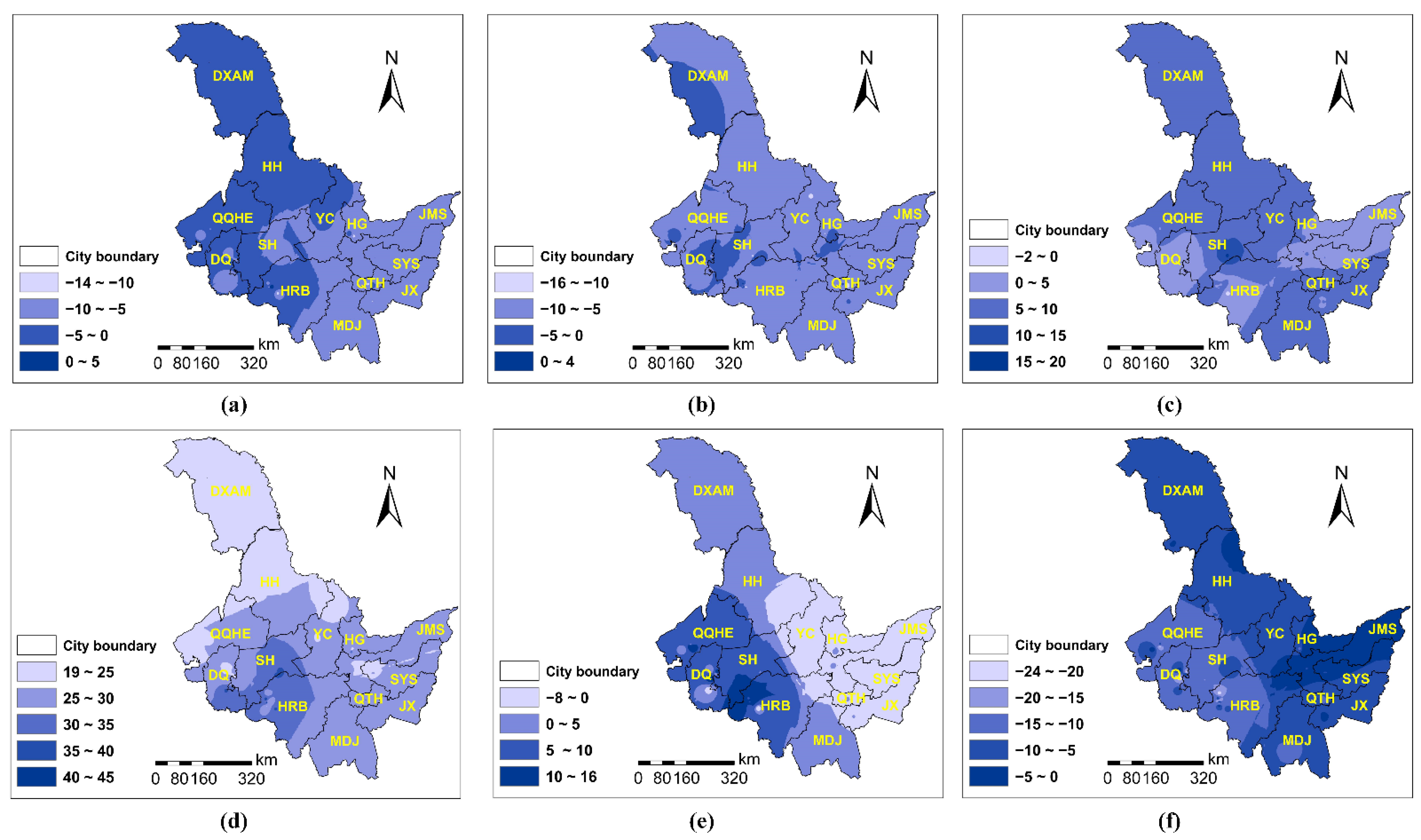
According to Figure 2, each PC factor had a difference influence in various locations for PM2.5. Temperature (Figure 2a) was the inhibitor of PM2.5 in most of Heilongjiang province. The inhibition was strong and obvious in the eastern area but weak in the west (e.g., Da Xing’an Mountain, Heihe, Qiqihar, Daqing, and Harbin). Wind speed (Figure 2b) primarily suppressed PM2.5, and the total inhibitory impact was comparable to temperature. Air pressure (Figure 2c) mostly promoted PM2.5, with a relative weak influence in Daqing, Harbin, Hegang, Jiamusi, and Shuangyashan. Atmospheric pollutants (Figure 2d) positively correlated with PM2.5, with three strata of correlations. The largest impact was observed the west of Harbin and the southern part around Daqing and Shuihua, whereas the smallest impact was observed in Da Xing’an Mountain, Heihe, and Qiqiha’er, and other places falling somewhere in the middle. Humidity (Figure 2e) had the ability to both enhance and inhibit PM2.5 levels. In the western cities, especially Harbin, Daqing, Suihua, and Qiqiha’er, humidity plays a role of promoting PM2.5; whereas in the eastern cities (e.g., Yichun, Hegang, Jiamusi, Shuangyashan, Qitaihe, and Jixi), it had a substantial negative effect. Vegetation cover (Figure 2f) obviously restricted PM2.5 concentration. The restriction trend decreased towards the east, with the smallest impact in Hegang, Jiamusi, and Shuangyashan.
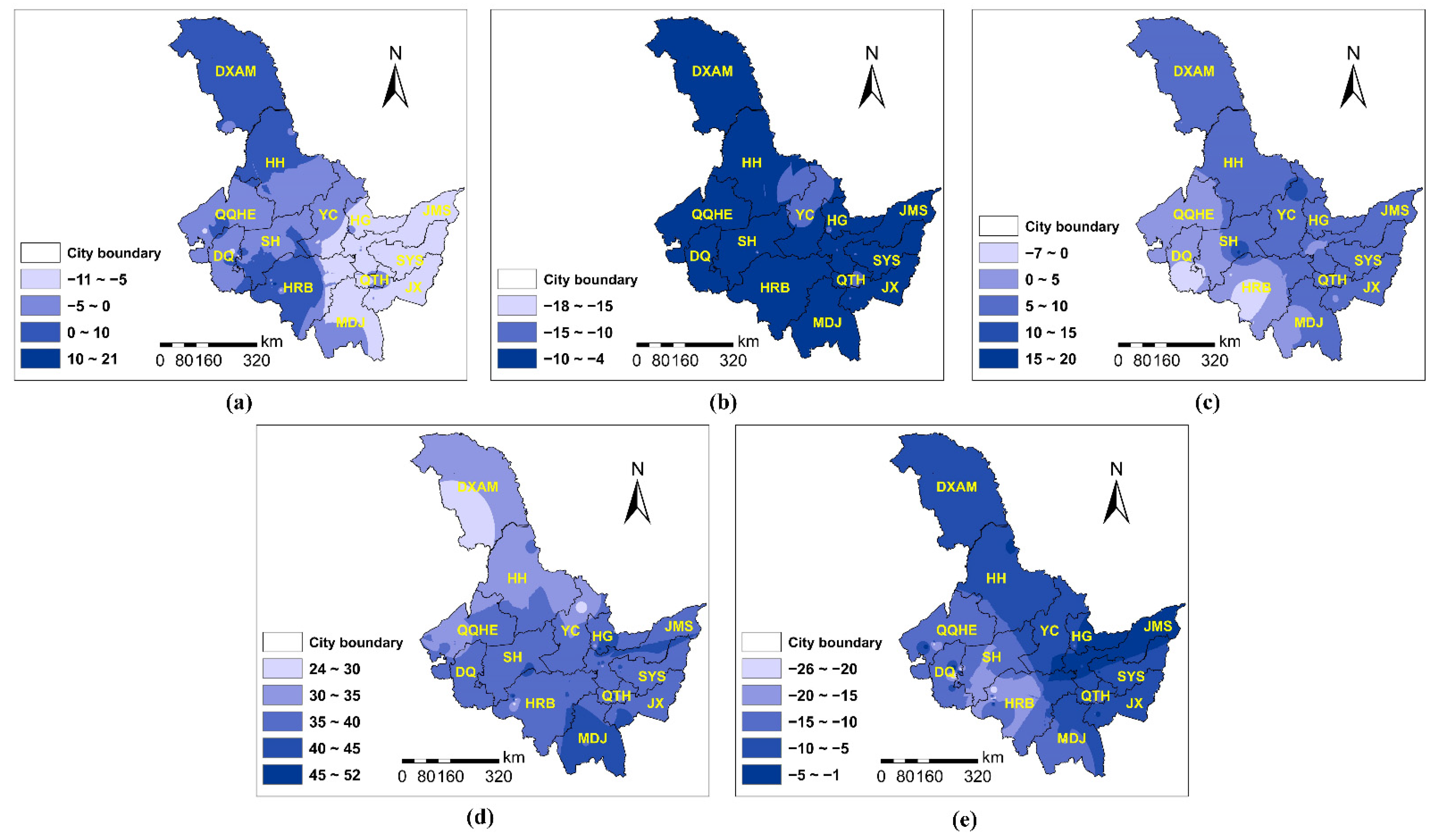
Similar to PM2.5, different PC factors had various influences on PM10 in space (Figure 3). However, the magnitude of parameter estimates for PM10 was much larger than that for PM2.5. Temperature (Figure 3a) could both enhance and inhibit PM10. Temperature tended to promote PM10 in Da Xing’an Mountain, Harbin, and Heihe. Whereas in other places, it played an inhibitory role. The inhibitory impact was stronger in the eastern area (i.e., Hegang, Jiamusi, Shuangyashan, Jixi) than the western area (e.g., Qiqiha’er, Daqing, Suihua, and Yichun). Wind speed (Figure 3b) had an inhibitory influence on PM10, and the inhibitory effect was fairly uniform across the region. Both pressure (Figure 3c) and atmospheric pollutants (Figure 3d) positively correlated with PM10. The positive correlation between PM10 and pressure tended to decrease from south to north, while its correlation with atmospheric pollutants presented the opposite trend. Vegetation cover (Figure 3e) inhibited PM10, with strong suppression in the cities of Qiqihar, Daqing, Suihua, Harbin, and Mudanjiang, and the suppression became weaker towards the east.

3.6. Temporal Characteristics of PCA-GTWR Parameter Estimates for PM

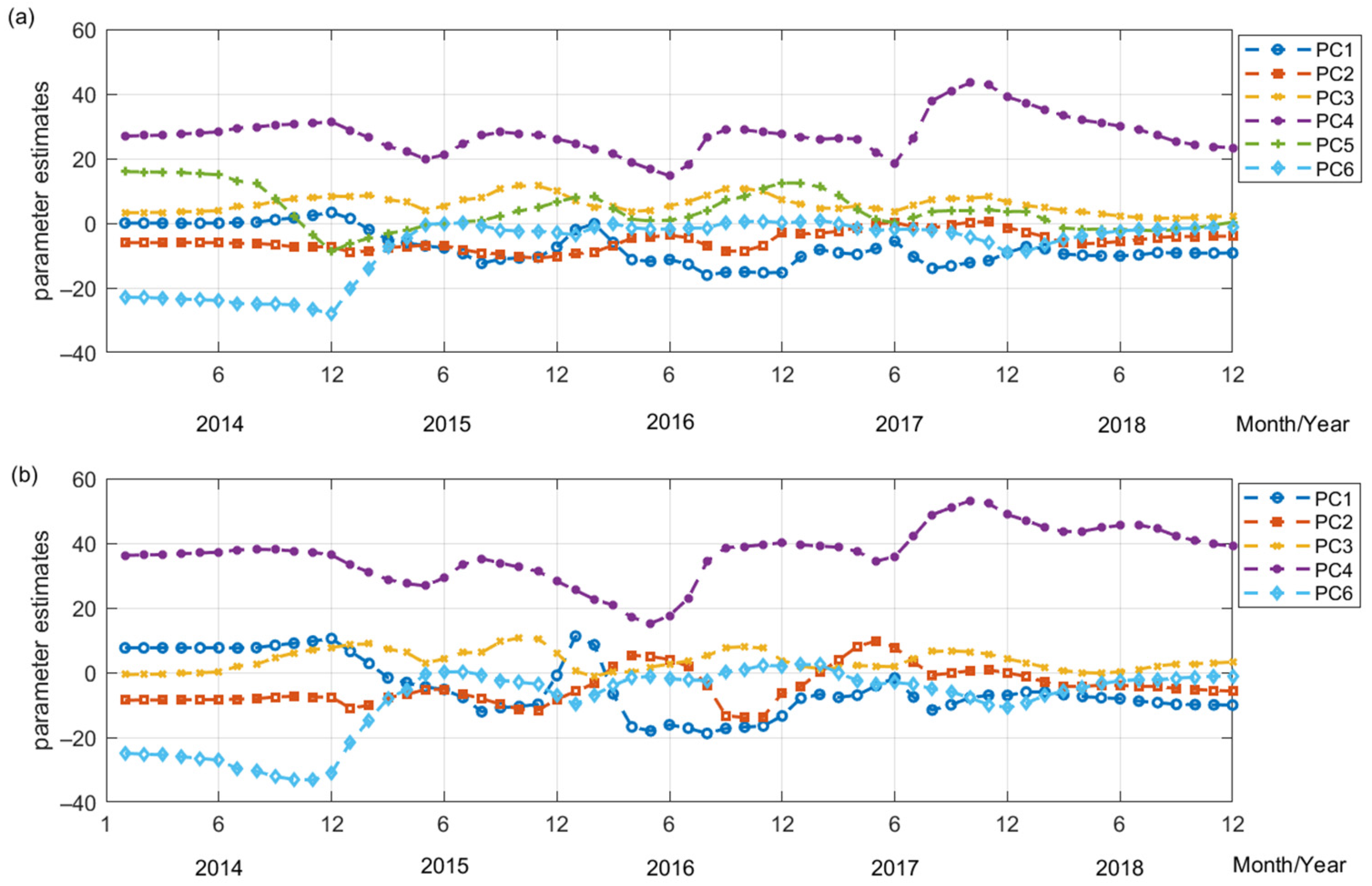
Figure 4 shows that influence of each PC on PM has temporal non-stationarity and periodicity, particularly PC3 (air pressure) and PC4 (atmospheric pollutants). For PM, the GTWR parameter estimates of PC3 and PC4 in the heating (i.e., winter) and non-heating (i.e., spring, summer, autumn seasons) periods differed and periodically changed during the course of a year: high in the heating season (usually from October to April next year) and low in the non-heating seasons. This is because the higher concentrations of atmospheric pressure and other air pollutants in winter are correlated with higher PM concentrations than those in summer.
The parameter estimates of PC1 (temperature) and PC2 (wind speed) has larger temporal periodicity for PM10 than PM2.5. The inhibitory effect of PC2 (wind speed) in autumn (September, October, and November) tends to be larger than that in other seasons. Due to the climate characteristics of Heilongjiang Province (cold temperate, and a temperate continental monsoon climate), the high wind speed in autumn tends to increase the inhibitory effect on PM. The inhibitory effect PC6 (vegetation coverage) on PM was obvious in 2014 but decrease and became stable afterwards. The impact of PC5 (humidity) on PM2.5 is not stable because PC5 is comprehensive factor that mainly controlled by daily average relative humility, daily cumulative humility and daily sun hours.

4. Discussion

4.1. The Key Influencing Factors of PM

Recently, many studies have investigated the connections between PM and a number of variables, including air pollutants, meteorological variables (such as temperature, wind speed, and relative humidity), the normalized difference vegetation index (NDVI) derived from satellite imagery, aerosol optical depth (AOD), human activities (such as transportation emission variables, the density of industrial plants, land use, GDP), and topographical factors and more [62,63,64,65,66,67]. Although it tends to improve PM predictions using more factors, it is difficult to remove multicollinearity among these factors and interpret the spatio-temporal relationship between PM and a number of factors. In this study, PCA was used to reduce the dimension of independent variables (i.e., from 20 original variables to 6 PCs) and remove the multicollinearity, and then OLS, GWR, TWR, and GTWR models were conducted based on the PCs to predict and explore the temporal and spatial heterogeneity of PM in Heilongjiang Province. Air pollutants (mainly SO2, NO2, and CO) represented by PC4 in this study have the largest influence on both PM2.5 and PM10 (see Table 2 and Table 3). Temperature expressed by PC1 had the second greatest impact on PM2.5, followed by air pressure (PC3), wind speed (PC2), vegetation cover (PC6), and humidity factor (PC5). Whereas the impacts of temperature, pressure, and vegetation cover on PM10 are roughly equivalent, followed by wind speed.
Although PM2.5 and PM10 are closely correlated [68], this study still shows some differences in the correlation between PM2.5/PM10 and the influenced factors. The main distinction is that, in contrast to PM2.5, the humidity factor (PC5) is not significant for PM10 and is eliminated in the global model. This may be because the humidity factor in this study is a combined variable of daily average relative humidity (positive), cumulative precipitation (positive), and sun hours (negative). It is challenging to demonstrate a meaningful relationship between the mixed variable and the comparatively large particle (PM10). The second factor contributing to the difference was wind speed. The dilution effect of wind speed on PM2.5 is stronger than that of PM10 due to the relatively light quality, which is consistent with the previous study [68].
In general, PM is positively related to other air pollutants (mainly SO2, NO2, and CO). It is similar to the finding that 5 criteria air pollutants (i.e., PM10, SO2, NO2, CO, O3) had a positive impact on PM2.5, except O3, in the previous study [4]. The concentration of PM reduces as the temperature (PC1) rises. When the temperature is high, the atmospheric tropospheric motion becomes more intense, resulting in the upward transport of PM, and the high temperature encourages Brownian particle motion, which is more favorable to diffusion [26]. Not surprisingly, the wind speed (PC2) has a negative effect on PM, which is consistent with previous studies [69,70]. This is because that the higher the wind speed, the stronger the particle dispersion capacity and the lower the particle concentration [71]. Atmospheric pressure (PC3) plays a positive role in increasing PM centration. When an area is subjected to high pressure, air convection is reduced, allowing contaminants to accumulate more easily, and vice versa [26,72]. The ability of the forest’s complex canopy structure to absorb particulate matter has long been recognized as a critical tool for controlling PM [73,74]. In this study, vegetation cover (PC6) also has a considerable inhibitory influence on PM. The absolute magnitude of the coefficient indicates that it has a significant impact on preventing PM increases. The explanation could be that vegetation intercepts and absorbs particulate matter via Brownian diffusion, interception, and gravity deposition [75,76].

4.2. Global and Local Models

In the constructed model, the problem of the PCA-OLS model is that it uses a global model to represent the relationship between dependent and independent variables, ignoring the spatial or temporal effect of the studied variables. This spatial or temporal effect (spatial/temporal autocorrelation and heterogeneity) may violate the assumption of independent observation or constant variance, resulting in the biases of estimates of standard errors and imprecision of coefficient estimates [77,78]. PCA-GWR was better than PCA-OLS by considering spatial heterogeneity (11% and 17% improvement of adjusted R 2 of PM2.5 and PM10, respectively). PCA-TWR was also superior to PCA-OLS by considering temporal heterogeneity (23% and 28% improvement of adjusted R 2 of PM2.5 and PM10, respectively). The temporal heterogeneity is more significant than the spatial heterogeneity due to the obvious seasonal variation of PM, which is consistent with the previous study [4]. The PCA-GTWR model that considers both temporal and spatial heterogeneity has the best performance (compared with PCA-OLS, the adjusted   R 2 increases by 25% and 31% for of PM2.5 and PM10, respectively). However, the improvements of PCA-GTWR from PCA-TWR are very limited, especially for PM2.5. It indicates that temporal information is more effective than spatial information for modeling PM based on PCA.

4.3. The Spatial and Temporal Distribution of PM Concentrations in Heilongjiang Province

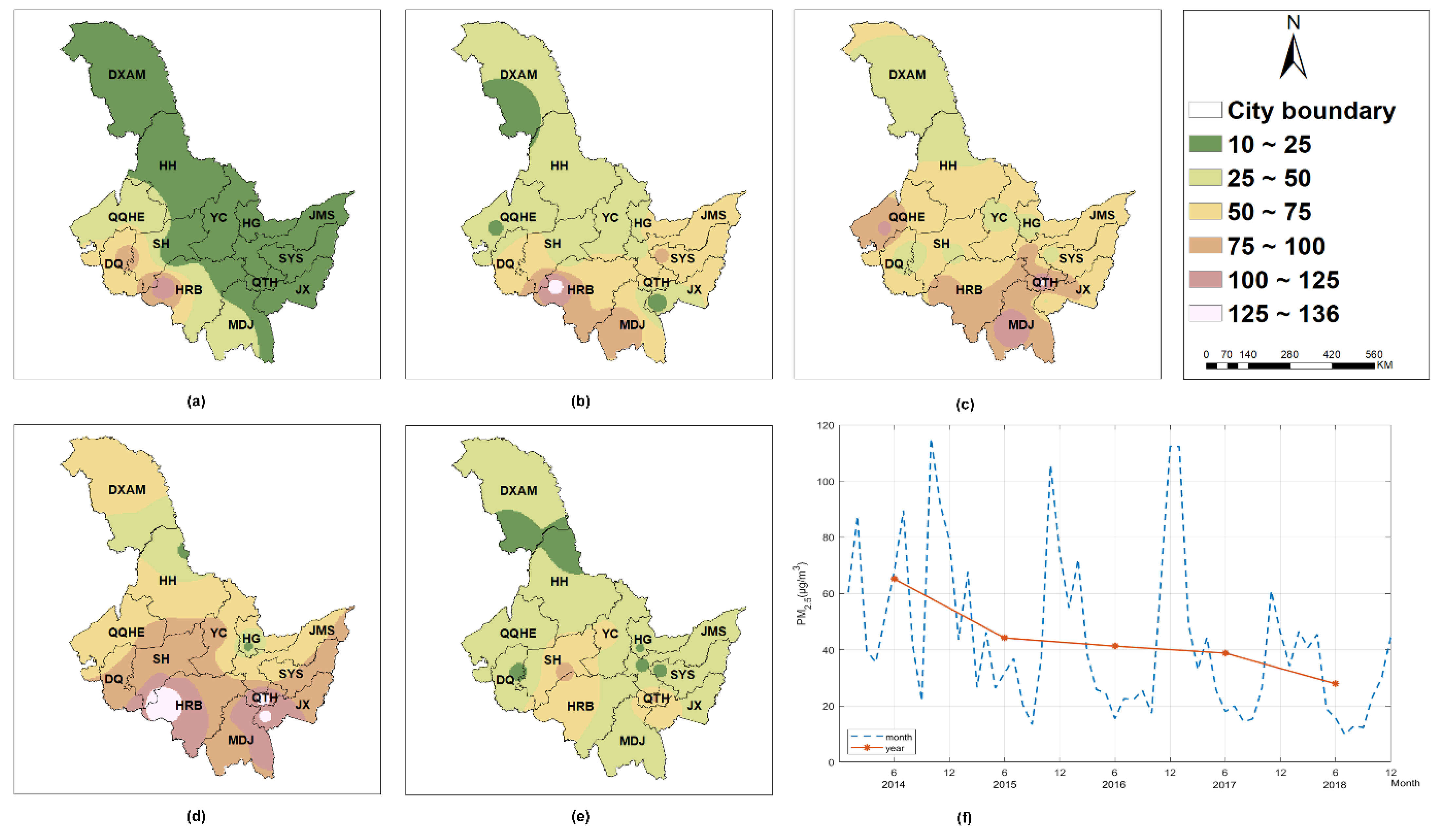
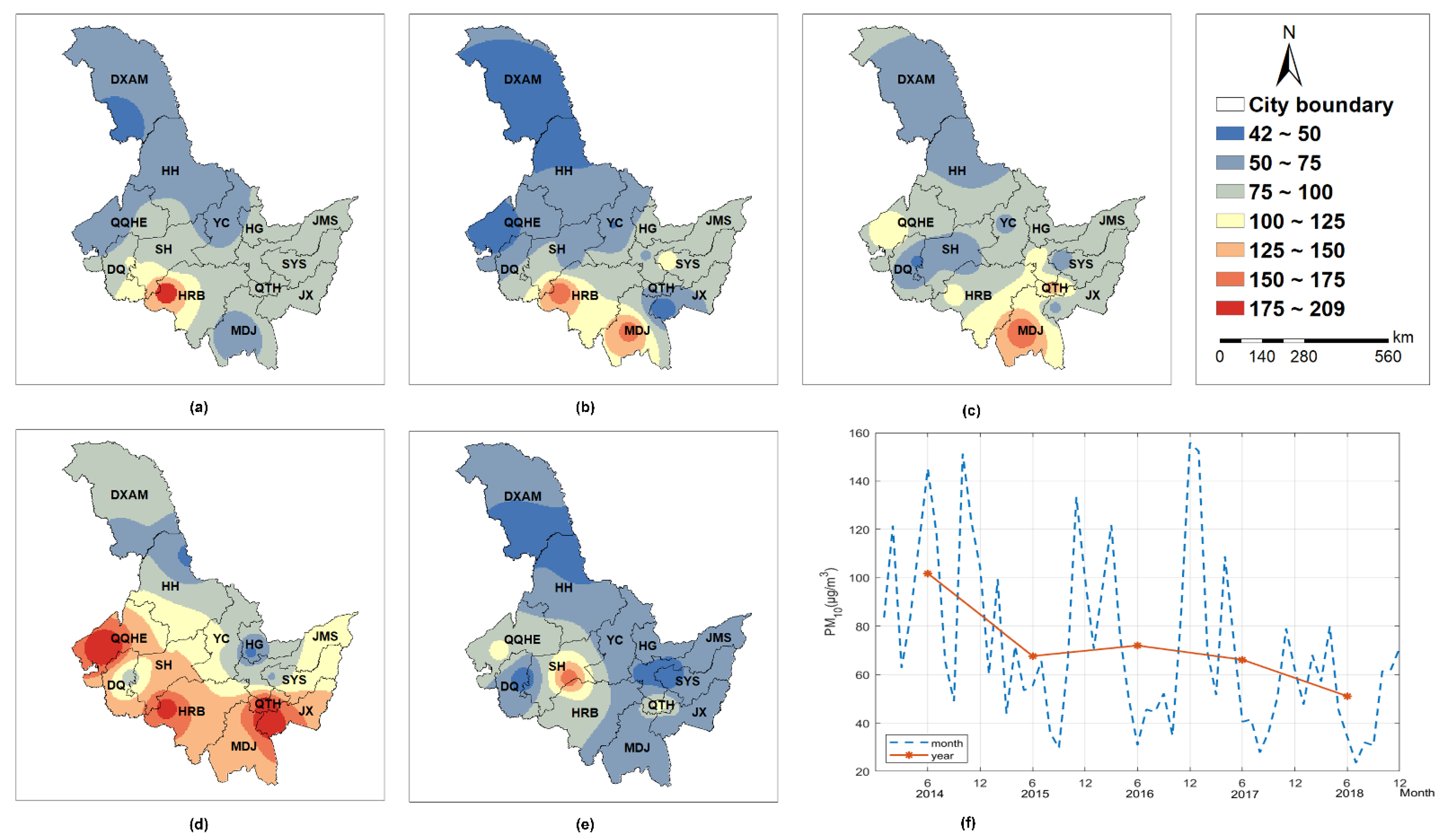
Heilongjiang Province is located in northern China and is noted for its high latitude and harsh winters. Heilongjiang Province is one of China’s largest provinces, with a north-south latitude range of approximately 10° and an east-west longitude range of approximately 4°. According to Figure 5 and Figure 6, the PM content in the southern area is significantly higher whereas that in the northern region is rather low due to the large population and coal burning in the south. Furthermore, the PM concentrations remained high from 2014 to 2017, especially in 2017. From spatio-temporal perspective, the hot spot of PM2.5 concentration gradually changed from southwestern (e.g., Harbin, Daqing) to southeastern cities (e.g., Harbin, Mudanjiang, Qitaihe, and Jixi). According to Figure 5f and Figure 6f, it can be seen that the temporal distribution of PM in Heilongjiang Province has heterogeneity and periodicity (high in winter and low in summer). The PM concentration in Heilongjiang Province grows dramatically during the heating season (from October to April next year). Coal-fired heating not only consumes energy but also harms the environment. However, due to the Heilongjiang Province’s policies (Air Pollution Prevention and Control Action Plan) [10], the downward trend of annual PM concentration is obvious, especially after 2017, which indicates the progress in the prevention and control of air pollution in Heilongjiang. In the future, Heilongjiang Province should implement a multi-energy integrated heating system that makes full use of renewable energy sources such as wind, water, and solar energy. Additionally, it is critical to consider advancing science and technology, discovering methods to store renewable energy, and even storing energy in the summer for use in winter heating. Finally, increasing the rate of urban greening, focusing on forest ecosystem protection, and enhancing the ecosystem’s ecological benefits are all necessary.

5. Conclusions

In this study, the spatial-temporal heterogeneity of PM (PM2.5 and PM10) concentration in Heilongjiang Province during 2014–2018 and the key impacting factors were investigated based on PCA-based local and global models. Six PCs with a contribution rate of 87% were selected, and each PC’s (PC1–PC6) meaning was obvious after rotation, representing the temperature, wind speed, air pressure, atmospheric pollution, humidity, and vegetation cover, respectively. According to the model assessment, all the PCA-based local models (PCA-GWR, PCA-TWR, and PCA-GTWR) were superior to the PCA-based global (PCA-OLS) model, in which PCA-GTWR performed the best. Air pollutants (mainly SO2, NO2, and CO) have the largest influence on both PM2.5 and PM10. The temperature has the second greatest impact on PM2.5, followed by air pressure, wind speed, vegetation cover, and humidity factor, whereas the impacts of temperature, pressure, and vegetation cover on PM10 are roughly equivalent, followed by wind speed. In general, PM is positively related to other air pollutants (mainly SO2, NO2, and CO) and air pressure, and negatively correlated to temperature, wind speed, and vegetation cover.
This study demonstrated that the temporal heterogeneity was more pronounced than the spatial heterogeneity of PM in Heilongjiang Province. This work provides temporal and spatial heterogeneity evidence of the relationship between PM and meteorological factors, air pollutants, and vegetation cover. Furthermore, this work addresses both excessive impact factors and temporal and spatial heterogeneity and provides a theoretical foundation for precise local government prevention and control.

Author Contributions

Conceptualization, L.F.; Data curation, Q.W. (Qingbin Wei); Formal analysis, L.F.; Investigation, L.F., Q.W. (Qibang Wang) and J.L.; Methodology, L.F. and J.L.; Project administration, Z.Z. and Q.W. (Qingbin Wei); Software, Q.W. (Qibang Wang); Supervision, Z.Z.; Validation, J.L.; Visualization, Q.W. (Qibang Wang); Writing—original draft, L.F.; Writing—review & editing, H.J., Z.Z. and Q.W. (Qingbin Wei). All authors have read and agreed to the published version of the manuscript.

Funding

This work was supported by the Key Laboratory of Forest Plant Ecology, Ministry of Education Northeast Forestry University (K2020C02), National Undergraduate Training Program for Innovation and Entrepreneurship (202110225060). This study was also supported by China Scholarship Council (CSC-No. 202006605008).

Institutional Review Board Statement

Not applicable.

Informed Consent Statement

Not applicable.

Data Availability Statement

The data that support the findings of this study are available from the corresponding author, (Z.Z. or Q.W.), upon reasonable request.

Conflicts of Interest

The authors declare no conflict of interest.

References

  1. Yin, H.; Brauer, M.; Zhang, J.; Cai, W.; Navrud, S.; Burnett, R.; Howard, C.; Deng, Z.; Kammen, D.M.; Schellnhuber, H.J.; et al. Population ageing and deaths attributable to ambient PM2.5 pollution: A global analysis of economic cost. Lancet Planet. Health 2021, 5, e356–e367. [Google Scholar] [CrossRef]
  2. Wang, H.; Zhang, L.; Cheng, I.; Yao, X.; Dabek-Zlotorzynska, E. Spatiotemporal trends of PM2.5 and its major chemical components at urban sites in Canada. J. Environ. Sci. 2020, 103, 1–11. [Google Scholar] [CrossRef] [PubMed]
  3. Choi, H.G.; Lee, C.H.; Yoo, D.M.; Min, C.; Park, B.; Kim, S.Y. Effects of short- and long-term exposure to air pollution and meteorological factors on Meniere’s disease. Sci. Rep. 2021, 11, 16063. [Google Scholar] [CrossRef] [PubMed]
  4. Wei, Q.; Zhang, L.; Duan, W.; Zhen, Z. Global and Geographically and Temporally Weighted Regression Models for Modeling PM2.5 in Heilongjiang, China from 2015 to 2018. Int. J. Environ. Res. Public Health 2019, 16, 5107. [Google Scholar] [CrossRef] [PubMed]
  5. Dominici, F.; Peng, R.D.; Bell, M.L.; Pham, L.; McDermott, A.; Zeger, S.L.; Samet, J.M. Fine Particulate Air Pollution and Hospital Admission for Cardiovascular and Respiratory Diseases. JAMA 2006, 295, 1127–1134. [Google Scholar] [CrossRef]
  6. Xing, Y.F.; Xu, Y.H.; Shi, M.H.; Lian, Y.X. The impact of PM2.5 on the human respiratory system. J. Thorac. Dis. 2016, 8, E69–E74. [Google Scholar]
  7. Apte, J.S.; Marshall, J.D.; Cohen, A.J.; Brauer, M. Addressing global mortality from ambient PM2.5. Environ. Sci. Technol. 2015, 49, 8057–8066. [Google Scholar] [CrossRef]
  8. Gu, K.; Zhou, Y.; Sun, H.; Dong, F.; Zhao, L. Spatial distribution and determinants of PM2.5 in China’s cities: Fresh evidence from IDW and GWR. Environ. Monit. Assess. 2020, 193, 15. [Google Scholar] [CrossRef]
  9. Wang, Y.; Yao, L.; Wang, L.; Liu, Z.; Ji, D.; Tang, G.; Zhang, J.; Sun, Y.; Hu, B.; Xin, J. Mechanism for the formation of the January 2013 heavy haze pollution episode over central and eastern China. Sci. China Earth Sci. 2013, 57, 14–25. [Google Scholar] [CrossRef]
  10. The State Council of China. Air Pollution Prevention and Control Action Plan. 10 September 2013. Available online: http://www.gov.cn/zhengce/content/2013-09/13/content_4561.htm (accessed on 19 June 2022).
  11. Li, G.; Fang, C.; Wang, S.; Sun, S. The effect of economic growth, urbanization, and industrialization on fine particulate matter (PM2.5) concentrations in China. Environ. Sci. Technol. 2016, 50, 11452–11459. [Google Scholar] [CrossRef]
  12. Lim, C.H.; Ryu, J.; Choi, Y.; Jeon, S.W.; Lee, W.K. Understanding global PM2.5 concentrations and their drivers in recent decades (1998–2016). Environ. Int. 2020, 144, 106011. [Google Scholar] [CrossRef]
  13. Liu, J.; Li, W.; Wu, J.; Liu, Y. Visualizing the intercity correlation of PM2.5 time series in the Beijing-Tianjin-Hebei region using ground-based air quality monitoring data. PLoS ONE 2018, 13, e0192614. [Google Scholar] [CrossRef]
  14. Wang, J.; Qu, W.; Li, C.; Zhao, C.; Zhong, X. Spatial distribution of wintertime air pollution in major cities over eastern China: Relationship with the evolution of trough, ridge and synoptic system over East Asia. Atmos. Res. 2018, 212, 186–201. [Google Scholar] [CrossRef]
  15. Yang, Y.; Christakos, G.; Yang, X.; He, J. Spatiotemporal characterization and mapping of PM2.5 concentrations in southern Jiangsu Province, China. Environ. Pollut. 2018, 234, 794–803. [Google Scholar] [CrossRef] [PubMed]
  16. Xu, F.; Xiang, N.; Higano, Y. How to reach haze control targets by air pollutants emission reduction in the Beijing-Tianjin-Hebei region of China? PLoS ONE 2017, 12, e0173612. [Google Scholar] [CrossRef]
  17. Zhang, H.; Wang, Y.; Hu, J.; Ying, Q.; Hu, X.-M. Relationships between meteorological parameters and criteria air pollutants in three megacities in China. Environ. Res. 2015, 140, 242–254. [Google Scholar] [CrossRef]
  18. Wu, Y. Source Apportionment of Atmospheric Particle Matter of Cities in Heilongjiang Province; China Environment Publishing House: Beijing, China, 2017; pp. 238–258. [Google Scholar]
  19. Theodosi, C.; Grivas, G.; Zarmpas, P.; Chaloulakou, A.; Mihalopoulos, N. Mass and chemical composition of size-segregated aerosols (PM2.5, PM10) over Athens, Greece: Local versus regional sources. Atmos. Chem. Phys. 2011, 11, 11895–11911. [Google Scholar] [CrossRef]
  20. Liu, G.; Li, J.; Wu, D.; Xu, H. Chemical composition and source apportionment of the ambient PM2.5 in Hangzhou, China. Particuology 2015, 18, 135–143. [Google Scholar] [CrossRef]
  21. Ye, B.; Ji, X.; Yang, H.; Yao, X.; Chan, C.; Cadle, S.; Chan, T.; Mulawa, P. Concentration and chemical composition of PM2.5 in Shanghai for a 1-year period. Atmos. Environ. 2003, 37, 499–510. [Google Scholar] [CrossRef]
  22. Cheng, Y.; Lee, S.; Gu, Z.; Ho, K.; Zhang, Y.; Huang, Y.; Chow, J.C.; Watson, J.G.; Cao, J.; Zhang, R. PM2.5 and PM10-2.5 chemical composition and source apportionment near a Hong Kong roadway. Particuology 2013, 18, 96–104. [Google Scholar] [CrossRef]
  23. Hajiloo, F.; Hamzeh, S.; Gheysari, M. Impact assessment of meteorological and environmental parameters on PM2.5 concentrations using remote sensing data and GWR analysis (case study of Tehran). Environ. Sci. Pollut. Res. 2018, 26, 24331–24345. [Google Scholar] [CrossRef] [PubMed]
  24. Chu, H.; Huang, B.; Lin, C.Y. Modeling the spatio-temporal heterogeneity in the PM10-PM2.5 relationship. Atmos. Environ. 2015, 102, 176–182. [Google Scholar] [CrossRef]
  25. Zou, B.; Fang, X.; Feng, H.; Zhou, X. Simplicity versus accuracy for estimation of the PM2.5 concentration: A comparison between LUR and GWR methods across time scales. J. Spat. Sci. 2019, 66, 279–297. [Google Scholar] [CrossRef]
  26. Li, Y.; Chen, Q.; Zhao, H.; Wang, L.; Tao, R. Variations in PM10, PM2.5 and PM1.0 in an Urban Area of the Sichuan Basin and Their Relation to Meteorological Factors. Atmosphere 2015, 6, 150–163. [Google Scholar] [CrossRef]
  27. Zhang, X.; Shi, M.; Li, Y.; Pang, R.; Xiang, N. Correlating PM2.5 concentrations with air pollutant emissions: A longitudinal study of the Beijing-Tianjin-Hebei region. J. Clean. Prod. 2018, 179, 103–113. [Google Scholar] [CrossRef]
  28. Suleiman, A.; Tight, M.; Quinn, A. Applying machine learning methods in managing urban concentrations of traffic-related particulate matter (PM10 and PM2.5). Atmos. Pollut. Res. 2018, 10, 134–144. [Google Scholar] [CrossRef]
  29. Czernecki, B.; Marosz, M.; Jędruszkiewicz, J. Assessment of Machine Learning Algorithms in Short-term Forecasting of PM10 and PM2.5 Concentrations in Selected Polish Agglomerations. Aerosol Air Qual. Res. 2021, 21, 200586. [Google Scholar] [CrossRef]
  30. Shen, J.; Valagolam, D.; McCalla, S. Prophet forecasting model: A machine learning approach to predict the concentration of air pollutants (PM2.5, PM10, O3, NO2, SO2, CO) in Seoul, South Korea. PeerJ 2020, 8, e9961. [Google Scholar] [CrossRef]
  31. Li, J.; Garshick, E.; Hart, J.E.; Li, L.; Shi, L.; Al-Hemoud, A.; Huang, S.; Koutrakis, P. Estimation of ambient PM2.5 in Iraq and Kuwait from 2001 to 2018 using machine learning and remote sensing. Environ. Int. 2021, 151, 106445. [Google Scholar] [CrossRef]
  32. Jiang, M.; Sun, W.; Yang, G.; Zhang, D. Modelling Seasonal GWR of Daily PM2.5 with Proper Auxiliary Variables for the Yangtze River Delta. Remote Sens. 2017, 9, 346. [Google Scholar] [CrossRef]
  33. Leung, Y.; Mei, C.-L.; Zhang, W.-X. Statistical Tests for Spatial Nonstationarity Based on the Geographically Weighted Regression Model. Environ. Plan. A Econ. Space 2000, 32, 9–32. [Google Scholar] [CrossRef] [Green Version]
  34. Huang, B.; Wu, B.; Barry, M. Geographically and temporally weighted regression for modeling spatio-temporal variation in house prices. Int. J. Geogr. Inf. Sci. 2010, 24, 383–401. [Google Scholar] [CrossRef]
  35. Zhao, C.-X.; Wang, Y.-Q.; Wang, Y.-J.; Zhang, H.-L.; Zhao, B.-Q. Temporal and spatial distribution of PM2.5 and PM10 pollution status and the correlation of particulate matters and meteorological factors during winter and spring in Beijing. Huan jing ke xue= Huanjing kexue 2014, 35, 418–427. [Google Scholar] [PubMed]
  36. Jin, J.-Q.; Du, Y.; Xu, L.-J.; Chen, Z.-Y.; Chen, J.-J.; Wu, Y.; Ou, C.-Q. Using Bayesian spatio-temporal model to determine the socio-economic and meteorological factors influencing ambient PM2.5 levels in 109 Chinese cities. Environ. Pollut. 2019, 254, 113023. [Google Scholar] [CrossRef] [PubMed]
  37. Kulsum, U.; Moniruzzaman, M. Quantifying the relationship of vegetation cover and air pollution: A spatiotemporal analysis of PM2.5 and NDVI in Greater Dhaka, Bangladesh. Jagannath Univ. J. Sci. 2021, 7, 54–63. [Google Scholar]
  38. Hughes, G. On the mean accuracy of statistical pattern recognizers. IEEE Trans. Inf. Theory 1968, 14, 55–63. [Google Scholar] [CrossRef]
  39. Dalponte, M.; Orka, H.O.; Gobakken, T.; Gianelle, D.; Naesset, E. Tree Species Classification in Boreal Forests with Hyperspectral Data. IEEE Trans. Geosci. Remote Sens. 2012, 51, 2632–2645. [Google Scholar] [CrossRef]
  40. Moore, B. Principal component analysis in linear systems: Controllability, observability, and model reduction. IEEE Trans. Autom. Control 1981, 26, 17–32. [Google Scholar] [CrossRef]
  41. Li, G.; Li, R.; Lu, Y.; Zhao, Y.; Yu, B. Using principal component analysis and geographic weighted regression methods to analyze AOD data. Bull. Surv. Mapp. 2018, 50–56. [Google Scholar] [CrossRef]
  42. Bizon, K.; Continillo, G.; Mancaruso, E.; Merola, S.S.; Vaglieco, B.M. POD-based analysis of combustion images in optically accessible engines. Combust. Flame 2010, 157, 632–640. [Google Scholar] [CrossRef]
  43. Maćkiewicz, A.; Ratajczak, W. Principal components analysis (PCA). Comput. Geosci. 1993, 19, 303–342. [Google Scholar] [CrossRef]
  44. Coussement, A.; Isaac, B.J.; Gicquel, O.; Parente, A. Assessment of different chemistry reduction methods based on principal component analysis: Comparison of the MG-PCA and score-PCA approaches. Combust. Flame 2016, 168, 83–97. [Google Scholar] [CrossRef] [Green Version]
  45. Parente, A.; Sutherland, J.C. Principal component analysis of turbulent combustion data: Data pre-processing and manifold sensitivity. Combust. Flame 2013, 160, 340–350. [Google Scholar] [CrossRef]
  46. Zheng, Y.; Li, S.; Kanran, T.; Ma, X.; Qian, R. Effect of forest coverage rate and other influencing factors on PM2.5-taking panel data model of 13 cities (districts) in Heilongjiang province as example. J. Northeast. For. Univ. 2020, 48, 64–70. [Google Scholar]
  47. GB 3095-2012; Ambient Air Quality Standards. Ministry of Environmental Protection of P.R. China: Beijing, China, 2012.
  48. Shu, Y.; Liu, Y.; Duan, Z.; Zhang, Y.; Chen, Z. A fast preprocessing algorithm for massive MODIS 1B data. In Geoinformatics 2007: Remotely Sensed Data and Information; SPIE: Bellingham, WA, USA, 2007. [Google Scholar]
  49. Xiong, X.; Barnes, W. An overview of MODIS radiometric calibration and characterization. Adv. Atmos. Sci. 2006, 23, 69–79. [Google Scholar] [CrossRef]
  50. Toutin, T. Review article: Geometric processing of remote sensing images: Models, algorithms and methods. Int. J. Remote Sens. 2004, 25, 1893–1924. [Google Scholar] [CrossRef]
  51. Telaar, J.; von Schönermark, M. Comparison of simplified algorithms for atmospheric corrections of MERIS data over land. In Proceedings of the 57th International Astronautical Congress, Valencia, Spain, 2–6 October 2006. [Google Scholar] [CrossRef]
  52. Huete, A.; Didan, K.; Miura, T.; Rodriguez, E.P.; Gao, X.; Ferreira, L.G. Overview of the radiometric and biophysical performance of the MODIS vegetation indices. Remote Sens. Environ. 2002, 83, 195–213. [Google Scholar] [CrossRef]
  53. Bro, R.; Smilde, A.K. Principal component analysis. Anal. Methods 2014, 6, 2812–2831. [Google Scholar] [CrossRef]
  54. Zhu, Z.; Li, B.; Zhao, Y.; Zhao, Z.; Chen, L. Socio-Economic Impact Mechanism of Ecosystem Services Value, a PCA-GWR Approach. Pol. J. Environ. Stud. 2020, 30, 977–986. [Google Scholar] [CrossRef]
  55. Choi, S.; Kim, B. Applying PCA to Deep Learning Forecasting Models for Predicting PM2.5. Sustainability 2021, 13, 3726. [Google Scholar] [CrossRef]
  56. Pulugurtha, S.S.; Mathew, S. Modeling AADT on local functionally classified roads using land use, road density, and nearest nonlocal road data. J. Transp. Geogr. 2021, 93, 103071. [Google Scholar] [CrossRef]
  57. Chris Brunsdon, A.S.F.; Charlton, M.E. Geographically weighted regression: A method for exploring spatial nonstationarity. Geogr. Anal. 1996, 28, 281–298. [Google Scholar] [CrossRef]
  58. Nilsson, P. Natural amenities in urban space—A geographically weighted regression approach. Landsc. Urban Plan. 2014, 121, 45–54. [Google Scholar] [CrossRef]
  59. Wu, B.; Li, R.; Huang, B. A geographically and temporally weighted autoregressive model with application to housing prices. Int. J. Geogr. Inf. Sci. 2014, 28, 1186–1204. [Google Scholar] [CrossRef]
  60. Fotheringham, A.S.; Charlton, M.E.; Brunsdon, C. Geographically Weighted Regression: A Natural Evolution of the Expansion Method for Spatial Data Analysis. Environ. Plan. A Econ. Space 1998, 30, 1905–1927. [Google Scholar] [CrossRef]
  61. Lu, B.; Charlton, M.; Harris, P.; Fotheringham, A.S. Geographically weighted regression with a non-Euclidean distance metric: A case study using hedonic house price data. Int. J. Geogr. Inf. Sci. 2013, 28, 660–681. [Google Scholar] [CrossRef]
  62. Li, L.; Zhang, J.; Qiu, W.; Wang, J.; Fang, Y. An ensemble spatiotemporal model for predicting PM2.5 concentrations. Int. J. Environ. Res. Public Health 2017, 14, 549. [Google Scholar] [CrossRef]
  63. Chelani, A.B. Estimating PM2.5 concentration from satellite derived aerosol optical depth and meteorological variables using a combination model. Atmos. Pollut. Res. 2018, 10, 847–857. [Google Scholar] [CrossRef]
  64. Zheng, C.; Zhao, C.; Zhu, Y.; Wang, Y.; Shi, X.; Wu, X.; Chen, T.; Wu, F.; Qiu, Y. Analysis of influential factors for the relationship between PM2.5 and AOD in Beijing. Atmos. Chem. Phys. 2017, 17, 13473–13489. [Google Scholar] [CrossRef]
  65. Liu, S.; Hua, S.; Wang, K.; Qiu, P.; Liu, H.; Wu, B.; Shao, P.; Liu, X.; Wu, Y.; Xue, Y.; et al. Spatial-temporal variation characteristics of air pollution in Henan of China: Localized emission inventory, WRF/Chem simulations and potential source contribution analysis. Sci. Total Environ. 2018, 624, 396–406. [Google Scholar] [CrossRef]
  66. Bai, Y.; Zeng, B.; Li, C.; Zhang, J. An ensemble long short-term memory neural network for hourly PM2.5 concentration forecasting. Chemosphere 2019, 222, 286–294. [Google Scholar] [CrossRef] [PubMed]
  67. Xue, T.; Zheng, Y.; Tong, D.; Zheng, B.; Li, X.; Zhu, T.; Zhang, Q. Spatiotemporal continuous estimates of PM2.5 concentrations in china, 2000–2016: A machine learning method with inputs from satellites, chemical transport model, and ground observations. Environ. Int. 2019, 123, 345–357. [Google Scholar] [CrossRef] [PubMed]
  68. Zhou, X.; Cao, Z.; Ma, Y.; Wang, L.; Wu, R.; Wang, W. Concentrations, correlations and chemical species of PM2.5/PM10 based on published data in China: Potential implications for the revised particulate standard. Chemosphere 2016, 144, 518–526. [Google Scholar] [CrossRef] [PubMed]
  69. Hu, Y.; Tian, L.; Hu, J. Preliminary study on the temporal distribution of PML2.5 pollution and influence of meteorological factors in Bengbu city. Meteorol. Environ. Res. 2020, 11, 9–16. [Google Scholar]
  70. Dai, W.; Gao, J.Q.; Wang, B.; Ouyang, F. Statistical analysis of weather effects on PM2.5. Adv. Mater. Res. 2012, 610–613, 1033–1040. [Google Scholar] [CrossRef]
  71. Bhaskar, B.V.; Mehta, V.M. Atmospheric Particulate Pollutants and their Relationship with Meteorology in Ahmedabad. Aerosol Air Qual. Res. 2010, 10, 301–315. [Google Scholar] [CrossRef]
  72. Akyüz, M.; Çabuk, H. Meteorological variations of PM2.5/PM10 concentrations and particle-associated polycyclic aromatic hydrocarbons in the atmospheric environment of Zonguldak, Turkey. J. Hazard. Mater. 2009, 170, 13–21. [Google Scholar] [CrossRef]
  73. Nguyen, T.; Yu, X.; Zhang, Z.; Liu, M.; Liu, X. Relationship between types of urban forest and PM2.5 capture at three growth stages of leaves. J. Environ. Sci. 2015, 27, 33–41. [Google Scholar] [CrossRef]
  74. Zhu, C.; Przybysz, A.; Chen, Y.; Guo, H.; Chen, Y.; Zeng, Y. Effect of spatial heterogeneity of plant communities on air PM10 and PM2.5 in an urban forest park in Wuhan, China. Urban For. Urban Green. 2019, 46, 126487. [Google Scholar] [CrossRef]
  75. Balczó, M.G.; Ruck, B. Numerical modeling of flow and pollutant dispersion in street canyons with tree planting. Meteorol. Z. 2009, 18, 197–206. [Google Scholar] [CrossRef]
  76. Popek, R.; Gawrońska, H.; Wrochna, M.; Gawroński, S.; Saebø, A. Particulate Matter on Foliage of 13 Woody Species: Deposition on Surfaces and Phytostabilisation in Waxes—A 3-Year Study. Int. J. Phytoremediation 2013, 15, 245–256. [Google Scholar] [CrossRef] [PubMed]
  77. Lu, J.; Zhang, L. Geographically Local Linear Mixed Models for Tree Height-Diameter Relationship. For. Sci. 2012, 58, 75–84. [Google Scholar] [CrossRef]
  78. Zhen, Z.; Li, F.; Liu, Z.; Liu, C.; Zhao, Y.; Ma, Z.; Zhang, L. Geographically local modeling of occurrence, count, and volume of downwood in Northeast China. Appl. Geogr. 2013, 37, 114–126. [Google Scholar] [CrossRef]
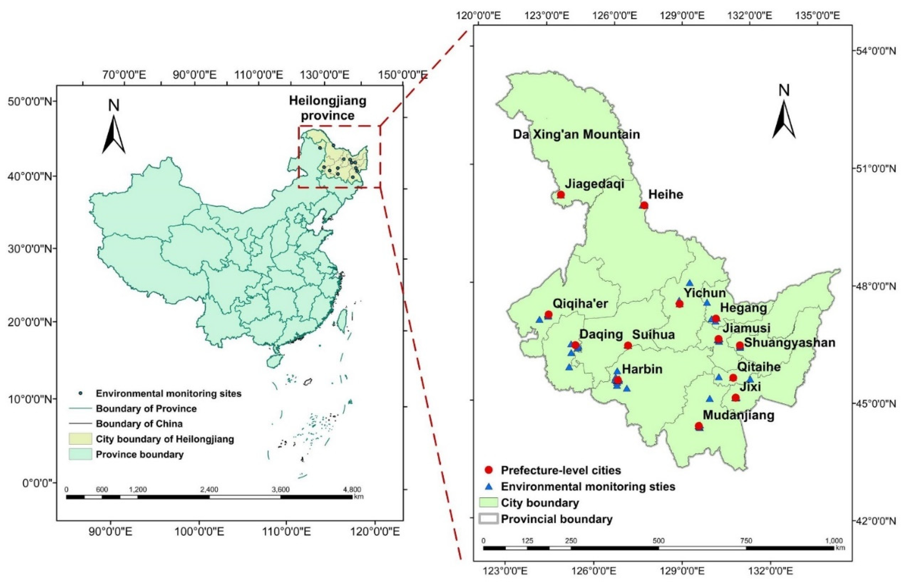
Figure 1. The location of Heilongjiang Province, People’s Republic of China (containing the Da Xing’an Mountain, Drawing review No: GS (2020)4619). Note: Jiagedaqi is a special residential neighborhood in which the Da Xing’an Mountain region’s environmental monitoring facility is located.
Ijerph 19 11627 g001
Figure 2. The PCA-GTWR parameter estimates of PM2.5 interpolated by Inverse Distance Weighted (IDW) method: (a) PC1 (temperature); (b) PC2 (wind speed); (c) PC3 (pressure); (d) PC4 (atmospheric pollutant); (e) PC5 (humidity); (f) PC6 (vegetation coverage). Note: HRB—Harbin; MDJ—Mudanjiang; QTH—Qitaihe; JX—Jixi; SYS—Shuangyashan; JMS—Jiamusi; HG—Hegang; YC—Yichun; SH—Suihua; DQ—Daqing; QQHE—Qiqiha’er; HH—Heihe; DXAM—Da Xing’an Mountain.
Ijerph 19 11627 g002
Figure 3. The PCA-GTWR parameter estimates of PM10 interpolated by IDW: (a) PC1 (temperature); (b) PC2 (wind speed); (c) PC3 (pressure); (d) PC4 (atmospheric pollutant); (e) PC6 (vegetation coverage). Note: HRB—Harbin; MDJ—Mudanjiang; QTH—Qitaihe; JX—Jixi; SYS—Shuangyashan; JMS—Jiamusi; HG—Hegang; YC—Yichun; SH—Suihua; DQ—Daqing; QQHE—Qiqiha’er; HH—Heihe; DXAM—Da Xing’an Mountain.
Ijerph 19 11627 g003
Figure 4. The temporal changes of PCA-GTWR parameter estimates for PM from 2014 to 2018: (a) PM2.5; (b) PM10. Note: PC1—temperature; PC2—wind speed; PC3—pressure; PC4—atmospheric pollutant; PC5—humidity; PC6—vegetation coverage.
Ijerph 19 11627 g004
Figure 5. The spatial and temporal distribution of PM2.5 (μg/m3) in Heilongjiang Province from 2014 to 2018: (a) 2014; (b) 2015; (c) 2016; (d) 2017; (e) 2018; (f) temporal trend of annual concentration. Note: HRB—Harbin; MDJ—Mudanjiang; QTH—Qitaihe; JX—Jixi; SYS—Shuangyashan; JMS—Jiamusi; HG—Hegang; YC—Yichun; SH—Suihua; DQ—Daqing; QQHE—Qiqiha’er; HH—Heihe; DXAM—Da Xing’an Mountain.
Ijerph 19 11627 g005
Figure 6. The spatial and temporal distribution of PM10 (μg/m3) in Heilongjiang Province from 2014 to 2018: (a) 2014; (b) 2015; (c) 2016; (d) 2017; (e) 2018; (f) temporal trend of annual concentration. Note: HRB—Harbin; MDJ—Mudanjiang; QTH—Qitaihe; JX—Jixi; SYS—Shuangyashan; JMS—Jiamusi; HG—Hegang; YC—Yichun; SH—Suihua; DQ—Daqing; QQHE—Qiqiha’er; HH—Heihe; DXAM—Da Xing’an Mountain.
Ijerph 19 11627 g006
Table 1. Descriptive statistics of the variables used in this study.
CategoryVariablesMinMeanMaxSDKurtosisSkewness
Dependent
variable
PM2.5 (μg/m3)4.0041.08262.0037.176.592.35
PM10 (μg/m3)10.0066.74341.0046.823.951.85
Air
pollutants
SO2 (μg/m3)2.0020.66191.0021.3413.803.03
NO2 (μg/m3)2.0028.37101.0016.151.941.31
CO (mg/m3)0.000.785.000.459.462.24
O3 (μg/m3)4.0073.71215.0029.011.130.92
Meteorological
factors
ARH0.240.620.940.13−0.13−0.37
HCP (mm)0.000.5023.641.7641.325.78
SH(h)0.007.8113.932.99−0.16−0.40
MaxP (hPa)951.36996.441029.0911.83−0.04−0.28
AP (hPa)947.56993.941026.4111.980.00−0.28
MinP (hPa)943.96991.081021.7012.130.02−0.31
MaxT (°C)−26.577.4736.0615.81−1.380.00
AT (°C)−36.471.1328.7015.57−1.33−0.02
MinT (°C)−43.67−4.8623.7215.31−1.25−0.01
MaxWS (m/s)1.775.5813.031.730.520.60
AWS (m/s)0.562.647.231.031.010.85
EWS (m/s)2.598.9720.602.880.120.49
MaxST (°C)−16.3317.3463.0621.19−1.390.24
AST (°C)−18.096.0136.3714.39−1.250.35
MinST (°C)−23.40−1.2223.3610.43−0.920.42
Vegetation coverageNDVI−0.31−0.070.780.129.082.73
Note: ARH—daily average relative humidity; HCP—daily cumulative precipitation; SH—daily sun hours; MaxP—daily maximum air pressure; AP—daily average air pressure; MinP—daily minimum air pressure; MaxT—daily maximum temperature; AT—daily average temperature; MinT—daily minimum temperature; MaxWS—daily maximum wind speed; AWS—daily average wind speed; EWS—daily extreme wind speed; MaxST—daily maximum surface temperature; AST—daily average surface temperature; MinST—daily minimum surface temperature.
Table 2. Principal component loadings of each PC after the maximum variance orthogonal rotation approach.
PCsPC1PC2PC3PC4PC5PC6
SO2 (μg/m3)−0.36−0.100.090.770.030.04
NO2 (μg/m3)−0.07−0.200.240.85−0.02−0.15
CO (mg/m3)−0.23−0.190.150.720.09−0.07
O3 (μg/m3)0.560.10−0.14−0.11−0.46−0.27
ARH0.03−0.460.020.140.740.08
HCP (mm)0.250.05−0.13−0.120.69−0.08
SH (h)0.49−0.060.00−0.18−0.690.09
MaxP (hPa)−0.27−0.020.940.18−0.04−0.06
AP (hPa)−0.26−0.080.940.17−0.04−0.05
MinP (hPa)−0.25−0.130.940.16−0.03−0.05
MaxT (°C)0.950.05−0.21−0.14−0.060.07
AT (°C)0.950.07−0.18−0.170.000.07
MinT (°C)0.940.10−0.16−0.180.090.07
MaxWS (m/s)0.020.97−0.11−0.12−0.04−0.01
AWS (m/s)0.000.940.02−0.15−0.060.00
EWS (m/s)0.120.95−0.13−0.16−0.060.01
MaxST (°C)0.940.01−0.19−0.17−0.120.06
AST (°C)0.960.00−0.19−0.14−0.020.07
MinST (°C)0.92−0.02−0.18−0.120.180.08
NDVI0.20−0.02−0.12−0.14−0.040.92
Meaning
of PCs
(Cumulative
Proportion)
Temperature
(40%)
Wind speed (57%)Pressure (67%)Atmospheric pollutants (75%)Humidity (82%)Vegetation cover
(87%)
Table 3. PCA-OLS model’s parameter estimations for PM (p< 0.01).
PM2.5Estimatet-Testp-ValuePM10Estimatet-Testp-Value
Intercept41.08136.27<2 × 10⁻¹⁶Intercept66.74162.13<2 × 10⁻¹⁶
PC1−7.39−24.50<2 × 10⁻¹⁶PC1−4.60−11.18<2 × 10⁻¹⁶
PC2−5.18−17.17<2 × 10⁻¹⁶PC2−1.83−4.458.81× 10−6
PC36.8522.72<2 × 10⁻¹⁶PC34.7211.47<2 × 10⁻¹⁶
PC426.4187.60<2 × 10⁻¹⁶PC433.4381.20<2 × 10⁻¹⁶
PC52.688.88<2 × 10⁻¹⁶PC6−4.67−11.33<2 × 10⁻¹⁶
PC6−3.03−10.05<2 × 10⁻¹⁶
R a 2 0.61 R a 2 0.54
AICc54,275.10 AICc57,976.60
Table 4. PCA-GWR, PCA-TWR, and PCA-GTWR parameter estimates of PM2.5 (the models are fitted by an adaptive neighbor selection algorithm).
ModelsVariablesMinMeanMaxSDKurtosisSkewnessModel Fitting Information
PCA-GWR (Num of Neighbors = 1041)intercept7.4335.7648.9515.09−0.64−1.04 R a 2 : 0.68
AICc: 53,295.1
PC1−13.61−5.75−0.184.29−1.37−0.25
PC2−6.46−3.88−0.981.81−1.420.14
PC32.0512.0126.148.40−1.020.70
PC415.1730.0537.555.740.68−0.95
PC5−2.743.638.862.88−0.830.11
PC6−21.18−7.64−1.486.06−1.13−0.71
PCA-TWR (Num of Neighbors = 595)intercept5.1839.6895.8713.874.500.87 R a 2 : 0.75
AICc: 51,804.3
PC1−25.34−3.7253.8312.886.661.98
PC2−14.13−4.178.214.40−0.010.09
PC3−12.005.0812.974.602.39−0.98
PC41.2022.7759.1611.461.070.67
PC5−9.795.3524.287.48−0.460.67
PC6−32.19−4.416.967.633.01−1.83
PCA-GTWR (Num of Neighbors = 595)intercept23.6441.8659.436.47−0.56−0.04 R a 2 : 0.76
AICc: 51,607.2
PC1−27.94−8.3522.705.560.490.37
PC2−19.60−4.6410.774.411.710.13
PC3−6.685.9026.564.832.500.85
PC48.6428.7951.438.41−0.240.43
PC5−13.173.3722.375.901.150.88
PC6−35.30−5.048.477.562.89−1.87
Table 5. PCA-GWR, PCA-TWR, and PCA-GTWR parameter estimates of PM10 (the models are fitted by an adaptive neighbor selection algorithm).
ModelsVariablesMinMeanMaxSDKurtosisSkewnessModel Fitting Information
PCA-GWR (Num of Neighbors = 937)intercept27.3962.5185.6519.74−0.880.26 R a 2 : 0.63
AICc: 56,894.4
PC1−12.54−2.019.206.36−0.890.08
PC2−8.22−0.146.694.75−1.340.06
PC3−1.7711.4525.948.29−0.650.11
PC423.4140.4445.956.132.020.08
PC6−20.11−8.67−2.414.64−0.830.06
PCA-TWR (Num of Neighbors = 602)intercept0.5666.42155.022.906.321.38 R a 2 : 0.71
AICc: 55,447.7
PC1−24.921.1284.1220.426.802.36
PC2−15.84−3.2221.888.360.460.87
PC3−21.353.7014.466.364.30−1.70
PC41.3630.6369.1012.930.700.38
PC6−32.82−5.3211.668.262.70−1.54
PCA-GTWR (Num of Neighbors = 595)intercept39.1269.63114.611.16−0.630.18 R a 2 : 0.73
AICc: 55,114.7
PC1−31.98−5.8345.628.412.030.79
PC2−21.94−2.8222.366.870.830.52
PC3−13.213.6527.616.361.160.18
PC49.2638.0460.4010.78−0.43−0.10
PC6−36.97−6.4412.978.812.37−1.60
Table 6. Comparison of PCA-OLS, PCA-GWR, PCA-TWR, PCA-GTWR.
ModelPM2.5PM10
AICc R a 2 RMSE
(μg/m3)
MAE (μg/m3)AICc R a 2 RMSE (μg/m3)MAE (μg/m3)
PCA-OLS54,275.100.6123.230.3057,976.600.5431.720.41
PCA-GWR53,295.100.6821.160.2756,892.600.6328.620.37
PCA-TWR51,804.300.7518.590.2455,836.900.6926.160.34
PCA-GTWR51,607.200.7618.200.2455,365.100.7125.040.33
Publisher’s Note: MDPI stays neutral with regard to jurisdictional claims in published maps and institutional affiliations.