
Spatiotemporal Variation in Ground Level Ozone and Its Driving Factors: A Comparative Study of Coastal and Inland Cities in Eastern China

Abstract
:
1. Introduction
2. Data and Methods
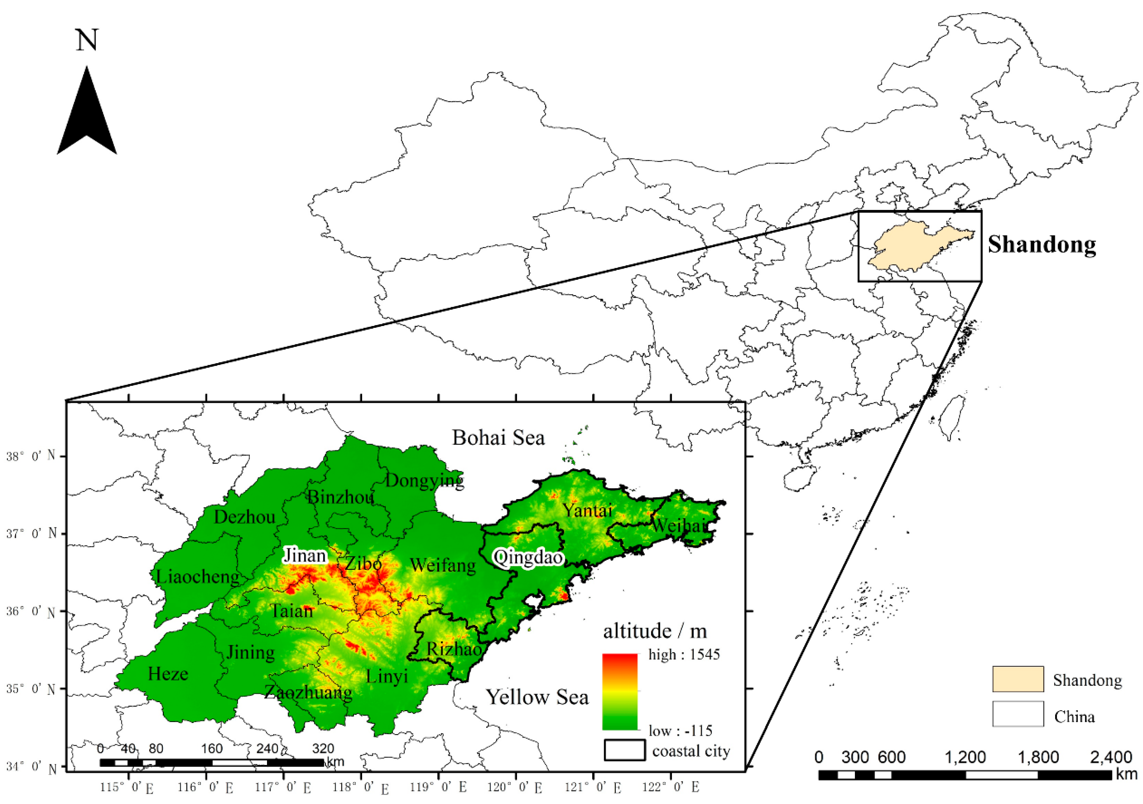
2.1. Study Area
2.2. O3 and Other Air Pollutants Data
2.3. Socioeconomic and Meteorological Data
2.4. Methods and Mechanism
2.4.1. GWR and MGWR
2.4.2. Wavelet Analysis
2.5. Choice of Two Typical Cities
3. Results and Discussion
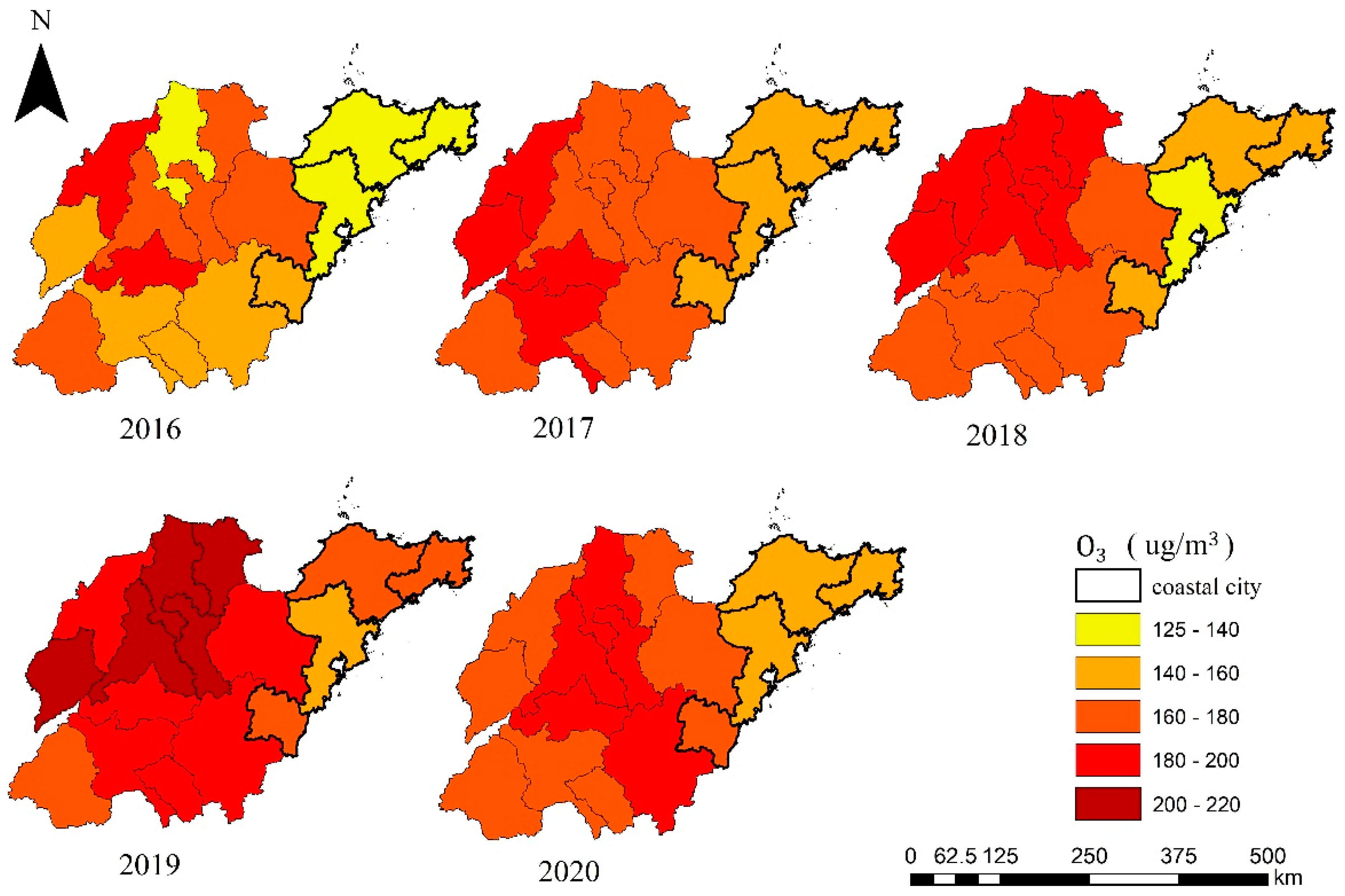
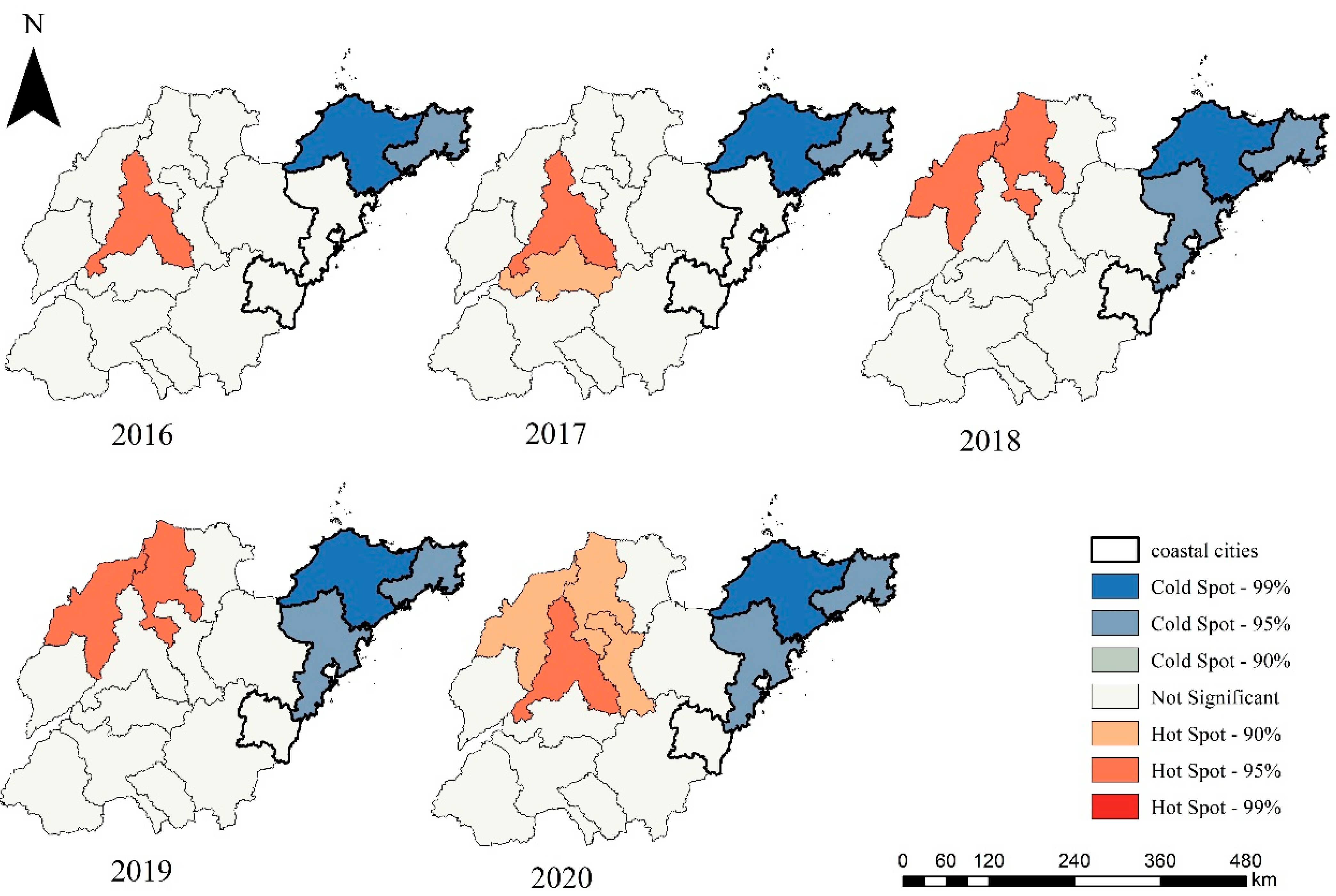
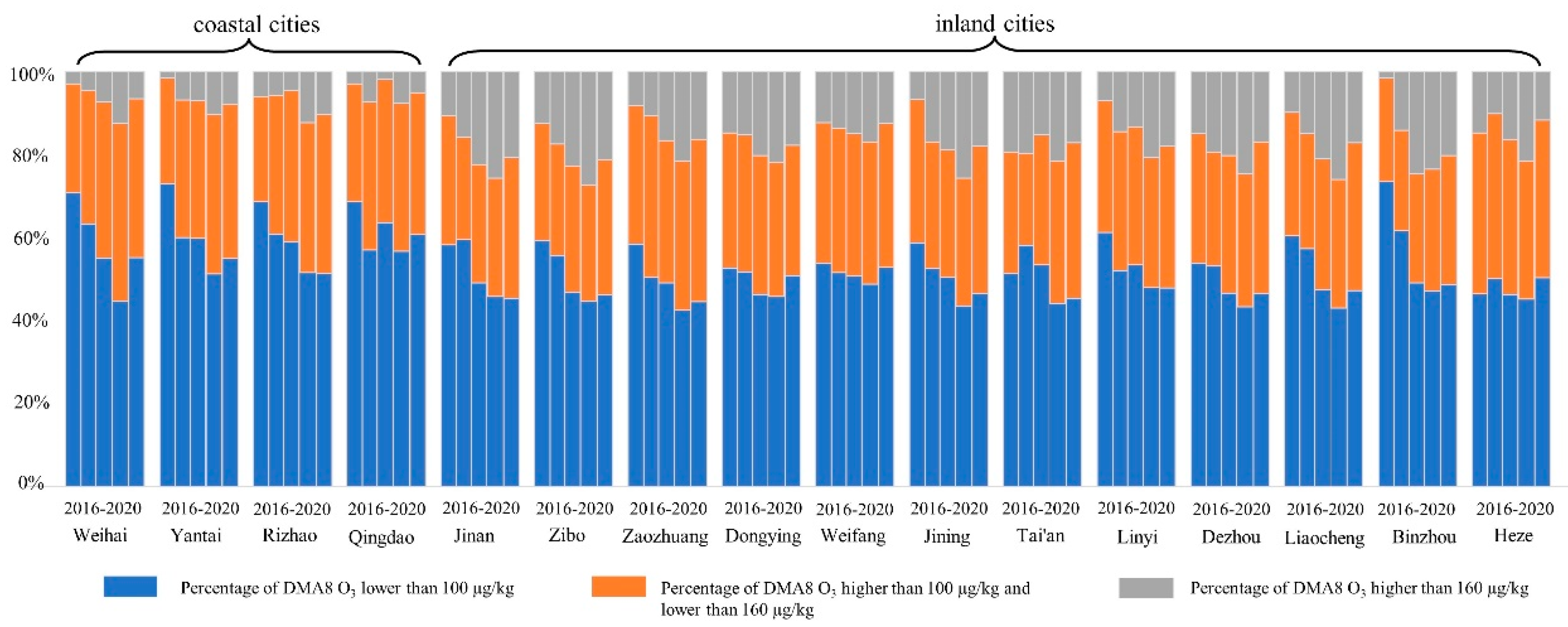
3.1. Spatiotemporal Distribution Characteristics of O3
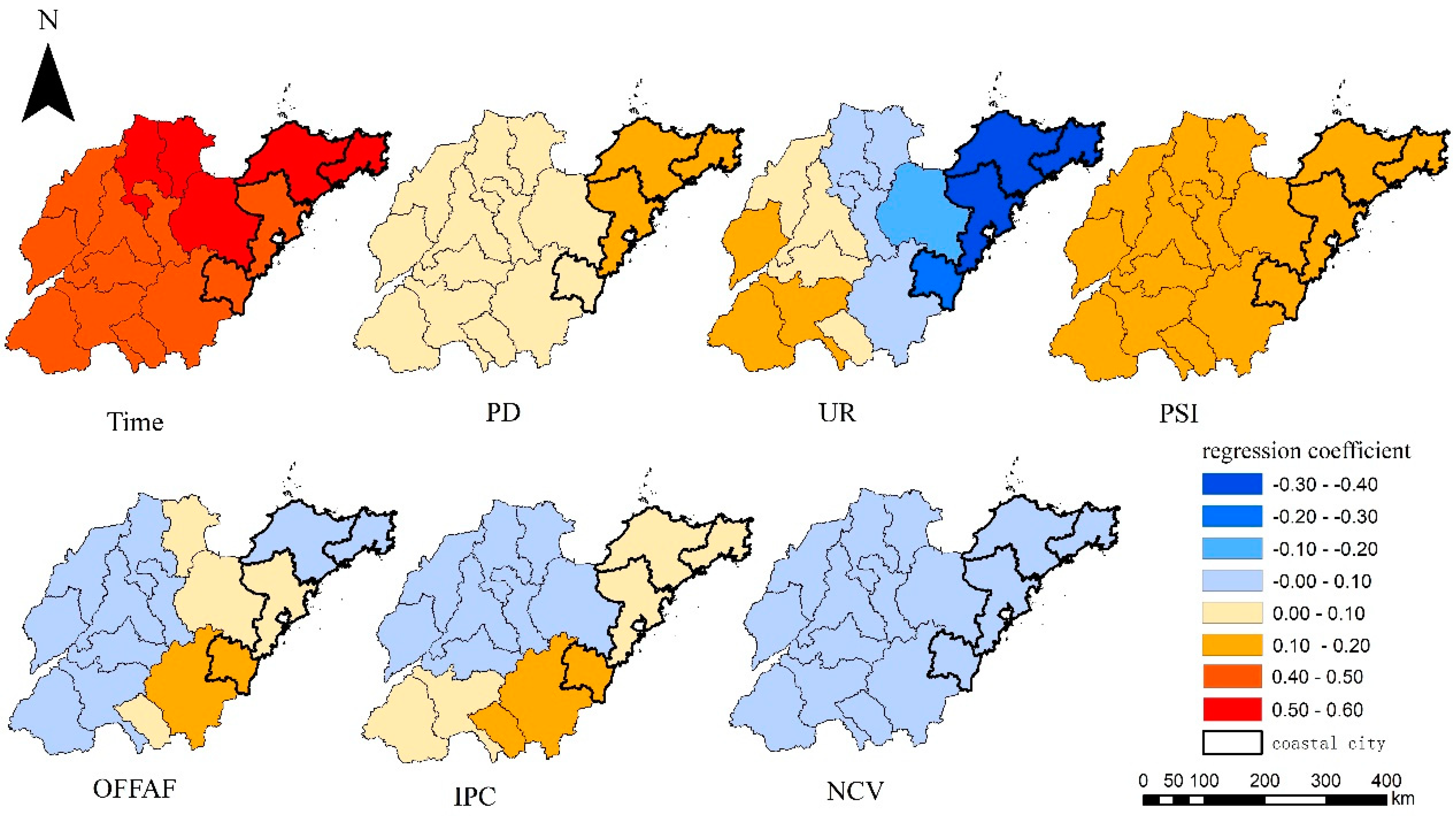
3.2. Socioeconomic Impacts
3.3. Impact of Other Air Pollutants and Meteorological Factors
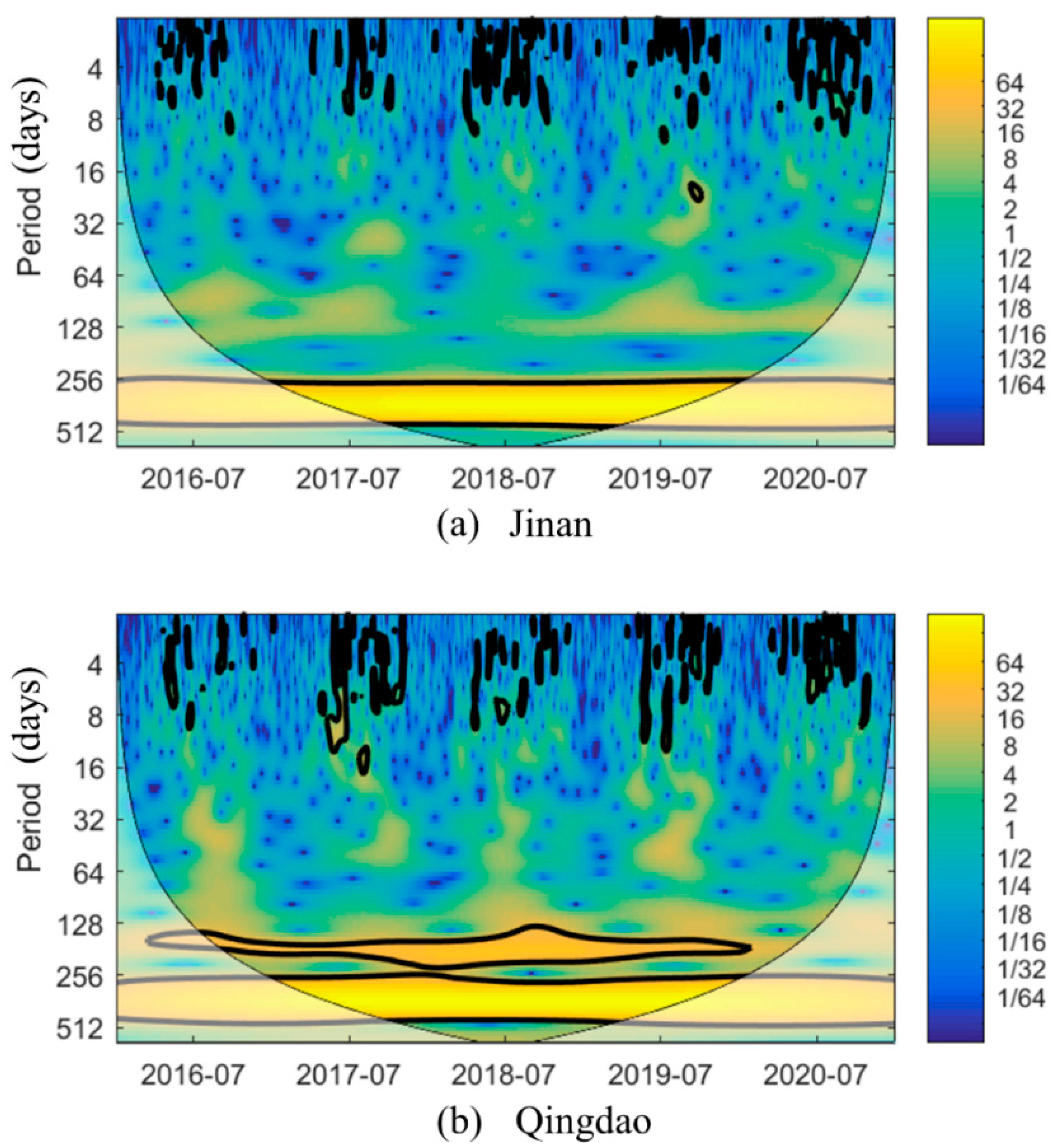
3.3.1. Wavelet Power Spectrum of O3 in Jinan and Qingdao
3.3.2. Wavelet Coherence Coefficient
3.3.3. Time Frequency and Phase Relationship between O3 and Other Air Pollutants
- (1)
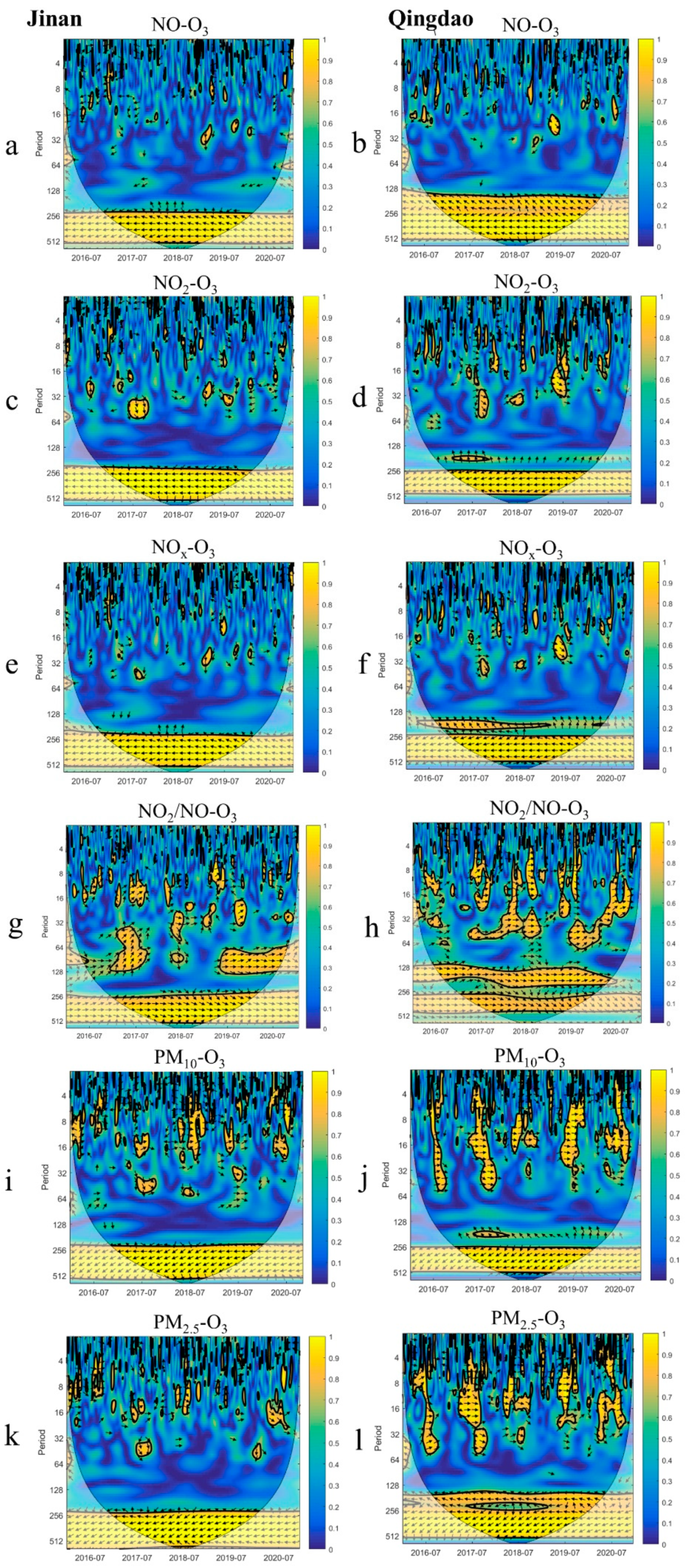
- NO, NO2, NOx, and NO2/NO. In the annual cycle, nitrogen oxides (including NO, NO2, and NOx) and O3 attained an inverse phase relationship, in which the value/phase of one parameter increased and that of the other parameter decreased (Figure 7). NO and O3 exhibited an inverse phase relationship with a short period (less than 14 days). This may occur as a result of NO titration reaction (R1). NO2 and O3, NOx and O3 mostly attained a positive phase relationship in summer and an inverse phase relationship in winter in the short period. O3 production in winter was generally in the NOx-saturated regime that high NOx concentration restrains O3 formation. Simultaneously, high NO emissions titration contributed to a reduction in O3 [11]. In summer, O3 was in the NOx-limited regime that the increase of NO2 was conducive to O3 formation (R2). Xia et al. (2021) similarly showed that the daily O3 concentration is higher when the daily NO2 concentration is higher in summer [36]. In addition to NOx, VOCs are also important precursors for O3 formation, which readily affect the variation of O3 concentration in winter [74,75,76]. However, VOCs were not regarded as an influencing factor in this paper. The unexplained part of the figure may be mainly attributed to VOCs.
- (2)
- PM10and PM2.5. Particulate matter (PM) (including PM10 and PM2.5) fluctuate frequently in winter and spring in Jinan and Qingdao. The phase trend of PM with O3 was inclined to the left during the annual cycle, indicating that PM and O3 exhibited an inverse phase relationship, and the change in O3 preceded that in PM (Figure 7). In the short term (1~30 days), PM2.5 and O3 revealed opposite phases in winter and spring but the same phase in summer. In winter and spring, the PM2.5 concentration was high due to the increase in energy consumption (heating). An ultrahigh PM2.5 concentration could lead to light radiation weakening, which could reduce O3 production. In addition, PM2.5 scavenges HO2 and NOx radicals, resulting in O3 reduction [78]. O3 production is high in summer due to the high temperatures and strong solar irradiation. The PM concentration was low in summer. When the PM2.5 concentration increases to a certain extent, this could enhance the photochemical reactions of O3 [36]. PM10 attained a similar periodic relationship with O3. In this study, the relationship between PM and O3 in summer was closer in coastal areas. This is consistent with the findings of Xia et al. (2021) that the daily maximum PM2.5 concentration has a greater impact on the daily maximum O3 concentration [36]. While Hu et al. (2021) and Wang et al. (2020) both showed that PM10 has a much greater impact on O3 than PM2.5 due to different data accuracy and study area [14,79].
3.3.4. Time Frequency and Phase Relationship between O3 and Meteorological Factors
- (1)
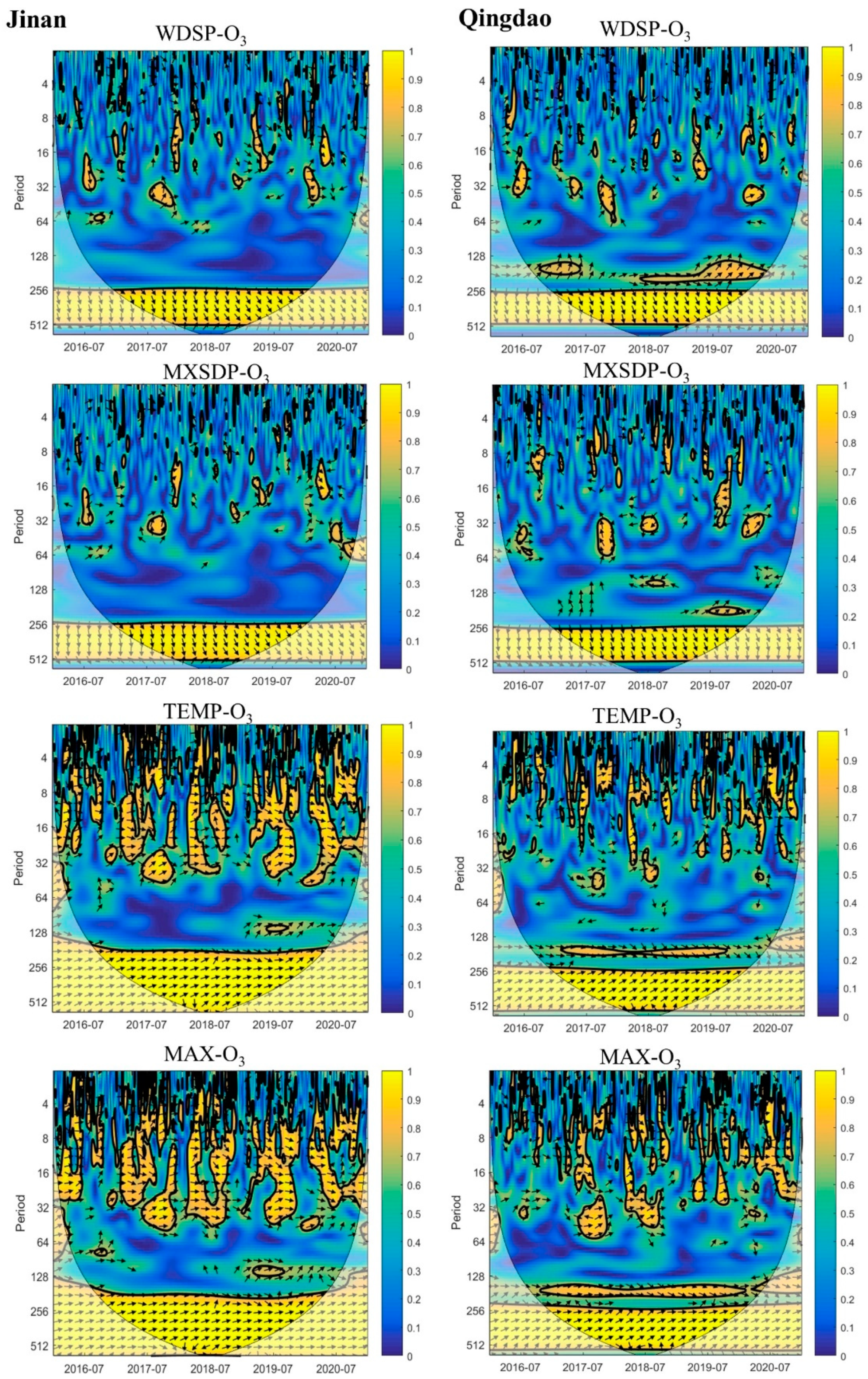
- Wind speed. Short-term (1~30 days) in-phase variation between WDSP and O3 in Jinan mostly occurred in winter and spring (Figure 8). The low temperature and low light in winter and spring lead to less O3 production. The observed increase in the O3 concentration probably occurred due to external transport. When the wind speed is high, exogenous O3 may be transported. This could cause an O3 increase in Jinan. Affected by sea and land winds, a complex correlation existed between WDSP and O3 in Qingdao. Sea breezes can not only lead to the accumulation of land air pollutants but can also lead to pollutant diffusion and transport [17]. This could result in the absence of obvious short-term coherence between WDSP and O3. In addition to WDSP, an obvious annual cycle was observed between MXSPD and O3. The corresponding phase relationship trended downward, indicating that the change in O3 preceded that in the wind speed. High wind speeds occur in winter and spring in both Qingdao and Jinan. In contrast, the O3 concentration is low in winter and spring.
- (2)
- Temperature. TEMP and O3 attained a high correlation over the annual cycle. Over the annual cycle, the trend was inclined upward, indicating that O3 change lagged behind that in TEMP. This is because the temperature rises slowly in spring, and the O3 concentration gradually increases thereafter. In the short term (within 14 days), mostly the same phase was observed. This indicates that O3 and TEMP simultaneously increased or decreased. A high temperature and notable radiation results in a high O3 production rate. The time–frequency relationship between O3 and MAX was the same as that between O3 and TEMP. However, the ARsq value between O3 and MAX (JN: 0.6283; QD: 0.5444) was higher than that between O3 and TEMP (JN: 0.5037; QD: 0.5185), which is consistent with Zhao et al. (2020) [3]. This may occur because the O3 concentration was the highest in the afternoon, and the highest temperature throughout the day also occurred in the afternoon [3.36]. Compared with Jinan, Qingdao attained a lower coherence between O3 and temperature.
3.4. Limitations
4. Conclusions
Supplementary Materials
Author Contributions
Funding
Institutional Review Board Statement
Informed Consent Statement
Data Availability Statement
Conflicts of Interest
References
- Kley, D.; Kleinmann, M.; Sanderman, H.; Krupa, S. Photochemical oxidants: State of the science. Environ. Pollut. 1999, 100, 19–42. [Google Scholar] [CrossRef]
- Lu, X.; Hong, J.; Zhang, L.; Cooper, O.R.; Schultz, M.G.; Xu, X.; Wang, T.; Gao, M.; Zhao, Y.; Zhang, Y. Severe Surface Ozone Pollution In Chinese: A Global Perspective. Environ. Sci. Technol. Lett. 2018, 5, 487–494. [Google Scholar] [CrossRef]
- Zhao, S.; Yin, D.; Yu, Y.; Kang, S.; Qin, D.; Dong, L. PM2.5 and O3 pollution during 2015–2019 over 367 Chinese cities: Spatiotemporal variations, meteorological and topographical impacts. Environ. Pollut. 2020, 264, 114694. [Google Scholar] [CrossRef] [PubMed]
- Ministry of Ecology and Environment of the People’s Republic of China (M.E.E.). Bulletin of the Ecological Environment of China in 2016. 2017. Available online: http://www.mee.gov.cn/hjzl/sthjzk/zghjzkgb/201706/P020170605833655914077.pdf (accessed on 26 May 2022). (In Chinese)
- Ministry of Ecology and Environment of the People’s Republic of China (M.E.E.). Bulletin of the Ecological Environment of China in 2017. 2018. Available online: https://www.mee.gov.cn/hjzl/sthjzk/zghjzkgb/201805/P020180531534645032372.pdf (accessed on 26 May 2022). (In Chinese)
- Ministry of Ecology and Environment of the People’s Republic of China (M.E.E.). Bulletin of the Ecological Environment of China in 2018. 2019. Available online: https://www.mee.gov.cn/hjzl/sthjzk/zghjzkgb/201905/P020190619587632630618.pdf (accessed on 26 May 2022). (In Chinese)
- Ministry of Ecology and Environment of the People’s Republic of China (M.E.E.). Bulletin of the Ecological Environment of China in 2019. 2020. Available online: http://www.mee.gov.cn/hjzl/sthjzk/zghjzkgb/202006/P020200602509464172096.pdf (accessed on 26 May 2022). (In Chinese)
- Ministry of Ecology and Environment of the People’s Republic of China (M.E.E.). Bulletin of the Ecological Environment of China in 2020. 2021. Available online: http://www.mee.gov.cn/hjzl/sthjzk/zghjzkgb/202105/P020210526572756184785.pdf (accessed on 26 May 2022). (In Chinese)
- Dong, Y.; Li, J.; Guo, J.; Jiang, Z.; Chu, Y.; Chang, L.; Yang, Y.; Liao, H. The impact of synoptic patterns on summertime ozone pollution in the North China Plain. Sci. Total Environ. 2020, 735, 139559. [Google Scholar] [CrossRef]
- Gong, C.; Liao, H.; Zhang, L.; Yue, X.; Dong, R.; Yang, Y. Persistent ozone pollution episodes in North China exacerbated by regional transport. Environ. Pollut. 2020, 265, 115056. [Google Scholar] [CrossRef]
- Li, K.; Jacob, D.J.; Liao, H.; Qiu, Y.; Shen, L.; Zhai, S.; Kelvin, H.; Bates, K.H.; Melissa, P.; Sulprizio, M.P.; et al. Ozone pollution in the North China Plain spreading into the late-winter haze season. Proc. Natl. Acad. Sci. USA 2021, 118, e2015797118. [Google Scholar] [CrossRef]
- Qin, Y.; Li, J.; Gong, K.; Wu, Z.; Chen, M.; Qin, M.; Huang, L.; Hu, J. Double high pollution events in the Yangtze River Delta from 2015 to 2019: Characteristics, trends, and meteorological situations. Sci. Total Environ. 2021, 792, 148349. [Google Scholar] [CrossRef]
- Zhang, X.; Feng, T.; Zhao, S.; Yang, G.; Quan Zhang, Q.; Qin, G.; Liu, L.; Long, X.; Sun, W.; Cao, G.; et al. Elucidating the impacts of rapid urban expansion on air quality in the Yangtze River Delta, China. Sci. Total Environ. 2021, 799, 149426. [Google Scholar] [CrossRef]
- Hu, M.; Wang, Y.; Wang, S.; Jiao, M.; Huang, G.; Xia, B. Spatial-temporal heterogeneity of air pollution and its relationship with meteorological factors in the Pearl River Delta, China. Atmos. Environ. 2021, 254, 118415. [Google Scholar] [CrossRef]
- Fang, T.; Zhu, Y.; Wang, S.; Xing, J.; Zhao, B.; Fan, S.; Li, M.; Yang, W.; Chen, Y.; Huang, R. Source impact and contribution analysis of ambient ozone using multi-modeling approaches over the Pearl River Delta region, China. Environ. Pollut. 2021, 289, 117860. [Google Scholar] [CrossRef]
- Wu, J.; Wang, Y.; Liang, J.; Yao, F. Exploring common factors influencing PM2.5 and O3 concentrations in the Pearl River Delta: Tradeoffs and synergies. Environ. Pollut. 2021, 285, 117138. [Google Scholar] [CrossRef]
- Zhao, D.; Xin, J.; Wang, W.; Jia, D.; Wang, Z.; Xiao, H.; Liu, C.; Zhou, J.; Tong, L.; Ma, M.; et al. Effects of the sea-land breeze on coastal ozone pollution in the Yangtze River Delta, China. Sci. Total Environ. 2022, 807, 150306. [Google Scholar] [CrossRef]
- Li, P.; Feng, Z.; Catalayud, V.; Yuan, X.; Xu, Y.; Paoletti, E. A meta-analysis on growth, physiological, and biochemical responses of woody species to ground-level ozone highlights the role of plant functional types. Plant Cell Environ. 2017, 40, 2369–2380. [Google Scholar] [CrossRef]
- Singh, A.A.; Agrawal, S.B. Tropospheric ozone pollution in India: Effects on crop yield and product quality. Environ. Sci. Pollut. Res. 2017, 24, 4367–4382. [Google Scholar] [CrossRef]
- Mills, G.; Sharps, K.; Simpson, D.; Pleijel, H.; Broberg, M.; Uddling, J.; Jaramillo, F.; Davies, W.J.; Dentener, F.; Berg, M.V.; et al. Ozone pollution will compromise efforts to increase global wheat production. Glob. Chang. Biol. 2018, 24, 3560–3574. [Google Scholar] [CrossRef]
- Yin, P.; Brauer, M.; Aaron, J.; Cohen, A.J.; Wang, H.; Li, J.; Burnett, R.T.; Stanaway, J.D.; Causey, K.; Larson, S.; et al. The effect of air pollution on deaths, disease burden, and life expectancy across China and its provinces, 1990–2017: An analysis for the Global Burden of Disease Study 2017. Lancet Planet. Health 2020, 4, e386–e398. [Google Scholar] [CrossRef]
- Lu, X.; Zhang, L.; Wang, X.; Gao, M.; Li, K.; Zhang, Y.; Yue, X.; Zhang, Y. Rapid Increases in Warm-Season Surface Ozone and Resulting Health Impact In Chinese since 2013. Environ. Sci. Technol. Lett. 2020, 7, 240–247. [Google Scholar] [CrossRef]
- Guan, Y.; Yang, X.; Wang, Y.; Zhang, N.; Chun, C. Long-term health impacts attributable to PM2.5 and ozone pollution In Chinese’s most polluted region during 2015–2020. J. Clean. Prod. 2021, 321, 128970. [Google Scholar] [CrossRef]
- Wu, S.; Mickley, L.J.; Jacob, D.J.; Rind, D.; Streets, D.G. Effects of 2000–2050 changes in climate and emissions on global tropospheric ozone and the policy-relevant background surface ozone in the United States. J. Geophys. Res. 2008, 113, D18312. [Google Scholar] [CrossRef] [Green Version]
- Jacob, D.J.; Winner, D.A. Effect of climate change on air quality. Atmos. Environ. 2009, 43, 51–63. [Google Scholar] [CrossRef] [Green Version]
- Ministry of Ecology and Environment of the People’s Republic of China (M.E.E.). 2020 Plan for against Volatile Organic Compounds. 2020. Available online: https://www.mee.gov.cn/xxgk2018/xxgk/xxgk03/202006/t20200624_785827.html (accessed on 28 May 2022). (In Chinese)
- Sillman, S. The relation between ozone, NOx and hydrocarbons in urban and polluted rural environments. Atmos. Environ. 1994, 33, 1821–1845. [Google Scholar] [CrossRef]
- Shao, M.; Zhang, Y.; Zeng, L.; Tang, X.; Zhang, J.; Zhong, L.; Wang, B. Ground-level ozone in the Pearl River Delta and the roles of VOC and NOx in its production. J. Environ. Manag. 2009, 90, 512–518. [Google Scholar] [CrossRef]
- Zhang, Q.; Yuan, B.; Shao, M.; Wang, X.; Lu, S.; Lu, K.; Wang, M.; Chen, L.; Chang, C.-C.; Liu, S.C. Variations of ground-level O3 and its precursors in Beijing in summertime between 2005 and 2011. Atmos. Chem. Phys. 2014, 14, 6089–6101. [Google Scholar] [CrossRef] [Green Version]
- Li, B.; Ho, S.S.H.; Gong, S.; Ni, J.; Li, H.; Han, L.; Yang, Y.; Qi, Y.; Zhao, D. Characterization of VOCs and their related atmospheric processes in a central Chinese city during severe ozone pollution periods. Atmos. Chem. Phys. 2019, 19, 617–638. [Google Scholar] [CrossRef] [Green Version]
- Li, H.; Ma, Y.; Duan, F.; Zhu, L.; Ma, T.; Yang, S.; Xu, Y.; Li, F.; Huang, T.; Kimoto, T.; et al. Stronger secondary pollution processes despite decrease in gaseous precursors: A comparative analysis of summer 2020 and 2019 in Beijing. Environ. Pollut. 2021, 279, 116923. [Google Scholar] [CrossRef] [PubMed]
- Xie, Y.; Cheng, C.; Wang, Z.; Wang, K.; Wang, Y.; Zhang, X.; Li, X.; Ren, L.; Liu, M.; Li, M. Exploration of O3-precursor relationship and observation-oriented O3 control strategies in a non-provincial capital city, southwestern China. Sci. Total Environ. 2021, 800, 149422. [Google Scholar] [CrossRef] [PubMed]
- Li, R.; Xu, M.; Li, M.; Chen, Z.; Zhao, N.; Gao, B.; Yao, Q. Identifying the spatiotemporal variations in ozone formation regimes across China from 2005 to 2019 based on polynomial simulation and causality analysis. Atmos. Chem. Phys. 2021, 21, 15631–15646. [Google Scholar] [CrossRef]
- Liu, P.; Song, H.; Wang, T.; Wang, F.; Li, X.; Miao, C.; Zhao, H. Effects of meteorological conditions and anthropogenic precursors on ground-level ozone concentrations in Chinese cities. Environ. Pollut. 2020, 262, 114366. [Google Scholar] [CrossRef]
- Yang, Z.; Yang, J.; Li, M.; Chen, J.J.; Ou, C.Q. Nonlinear and lagged meteorological effects on daily levels of ambient PM2.5 and O3: Evidence from 284 Chinese cities. J. Clean. Prod. 2021, 278, 123931. [Google Scholar] [CrossRef]
- Xia, N.; Du, E.; Guo, Z.; Vries, W.D. The diurnal cycle of summer tropospheric ozone concentrations across Chinese cities: Spatial patterns and main drivers. Environ. Pollut. 2021, 286, 117547. [Google Scholar] [CrossRef]
- Liang, D.; Wang, Y.Q.; Wang, Y.J.; Ma, C. National air pollution distribution In Chinese and related geographic, gaseous pollutant, and socio-economic factors. Environ. Pollut. 2019, 250, 998–1009. [Google Scholar] [CrossRef]
- Zhao, H.; Guo, S.; Zhao, H. Characterizing the Influences of Economic Development, Energy Consumption, Urbanization, Industrialization, and Vehicles Amount on PM2.5 Concentrations of China. Sustainability 2018, 10, 2574. [Google Scholar] [CrossRef]
- Jin, J.Q.; Du, Y.; Xu, L.J.; Chen, Z.Y.; Chen, J.J.; Wu, Y.; Ou, C.Q. Using Bayesian spatio-temporal model to determine the socioeconomic and meteorological factors influencing ambient PM2.5 levels in 109 Chinese cities. Environ. Pollut. 2019, 254, 113023. [Google Scholar] [CrossRef]
- Allen, R.J.; Hassan, T.; Randles, C.A.; Su, H. Enhanced land–sea warming contrast elevates aerosol pollution in a warmer world. Nat. Clim. Chang. 2019, 9, 300–305. [Google Scholar] [CrossRef]
- Fotheringham, A.S.; Yang, W.B.; Kang, W. Multiscale geographically weighted regression (MGWR). Ann. Am. Assoc. Geogr. 2017, 107, 1247–1265. [Google Scholar] [CrossRef]
- Guo, B.; Wang, X.; Pei, L.; Su, Y.; Zhang, D.; Wang, Y. Identifying the spatiotemporal dynamic of PM2.5 concentrations at multiple scales using geographically and temporally weighted regression model across China during 2015–2018. Sci. Total Environ. 2021, 751, 141765. [Google Scholar] [CrossRef]
- Zeng, C.; Yang, L.; Zhu, A.X.; Rossiter, D.G.; Liu, J.; Liu, J.; Qin, C.; Wang, D. Mapping soil organic matter concentration at different scales using a mixed geographically weighted regression method. Geoderma 2016, 281, 69–82. [Google Scholar] [CrossRef]
- Wu, T.; Zhou, L.; Jiang, G.; Meadows, M.E.; Zhang, J.; Pu, L.; Wu, C.; Xie, X. Modelling Spatial Heterogeneity in the Effects of Natural and Socioeconomic Factors, and Their Interactions, on Atmospheric PM2.5 Concentrations In Chinese from 2000–2015. Remote Sens. 2021, 13, 2152. [Google Scholar] [CrossRef]
- Zhan, D.; Zhang, Q.; Xu, X.; Zeng, C. Spatiotemporal distribution of continuous air pollution and its relationship with socioeconomic and natural factors In Chinese. Int. J. Environ. Res. Public Health 2022, 19, 6635. [Google Scholar] [CrossRef]
- Lau, K.M.; Weng, H. Climate Signal Detection Using Wavelet Transform: How to Make a Time Series Sing. Bull. Am. Meteorol. Soc. 1995, 76, 2391–2402. [Google Scholar] [CrossRef] [Green Version]
- Torrence, C.; Compo, C.P. A Practical Guide to Wavelet Analysis. Bull. Am. Meteorol. Soc. 1998, 79, 61–78. [Google Scholar] [CrossRef] [Green Version]
- Yi, H.; Shu, H. The improvement of the Morlet wavelet for multi-period analysis of climate data. Comptes Rendus Geosci. 2012, 344, 483–497. [Google Scholar] [CrossRef]
- Ng, E.K.W.; Chan, J.C.L. Geophysical Applications of Partial Wavelet Coherence and Multiple Wavelet Coherence. J Atmos. Ocean Technol. 2012, 29, 1845–1853. [Google Scholar] [CrossRef]
- Hu, W.; Si, B.C. Technical note: Multiple wavelet coherence for untangling scale-specific and localized multivariate relationships in geosciences. Earth Syst. Sci. 2016, 20, 3183–3191. [Google Scholar] [CrossRef] [Green Version]
- Cheng, Q.; Zhong, F.; Wang, P. Baseflow dynamics and multivariate analysis using bivariate and multiple wavelet coherence in an alpine endorheic river basin (Northwest China). Sci. Total Environ. 2021, 772, 145013. [Google Scholar] [CrossRef]
- Bilgili, F.; Lorente, D.B.; Kuşkaya, S.; Ünlü, F.; Gençoģlu, P.; Rosha, P. The role of hydropower energy in the level of CO2 emissions: An application of continuous wavelet transform. Renew. Energy 2021, 178, 283–294. [Google Scholar] [CrossRef]
- Trott, C.B.; Subrahmanyam, B.; Washburn, C.E. Investigating the Response of Temperature and Salinity in the Agulhas Current Region to ENSO Events. Remote Sens. 2021, 13, 1829. [Google Scholar] [CrossRef]
- Mensi, W.; Rehman, M.U.; Maitra, D.; Al-Yahyaee, K.H.; Vo, X.V. Oil, natural gas and BRICS stock markets: Evidence of systemic risks and co-movements in the time-frequency domain. Resour. Policy 2021, 72, 102062. [Google Scholar] [CrossRef]
- Tankanag, A.V.; Grinevich, A.A.; Kirilina, T.V.; Krasnikov, G.V.; Piskunova, G.M.; Chemeris, N.K. Wavelet phase coherence analysis of the skin blood flow oscillations in human. Microvasc. Res. 2014, 95, 53–59. [Google Scholar] [CrossRef]
- Rahman, M.S.; Azad, M.A.; Hasanuzzaman, M.; Salam, R.; Islam, A.R.; Rahman, M.M.; Hoque, M.M. How air quality and COVID-19 transmission change under different lockdown scenarios? A case from Dhaka city, Bangladesh. Sci. Total Environ. 2021, 762, 143161. [Google Scholar] [CrossRef]
- Ministry of Ecology and Environment of the People’s Republic of China (M.E.E.). Technical Regulation for Ambient Air Quality Assessment (on Trial) (HJ 663—2013). 2013. Available online: https://www.mee.gov.cn/ywgz/fgbz/bz/bzwb/jcffbz/201309/W020131105548549111863.pdf (accessed on 27 September 2021). (In Chinese)
- Ministry of Ecology and Environment of the People’s Republic of China (M.E.E.). Technical Regulation for Selection of Ambient Air Quality Monitoring Stations (on Trial) (HJ 664—2013). 2013. Available online: https://www.mee.gov.cn/ywgz/fgbz/bz/bzwb/jcffbz/201309/W020131105548727856307.pdf (accessed on 27 September 2021). (In Chinese)
- Ministry of Ecology and Environment of the People’s Republic of China (M.E.E.). Ambient Air Quality Standards (GB 3095-2012). 2012. Available online: https://www.mee.gov.cn/ywgz/fgbz/bz/bzwb/dqhjbh/dqhjzlbz/201203/W020120410330232398521.pdf (accessed on 25 September 2021). (In Chinese)
- Shandong Province Bureau of Statistics (SPBS). Shandong Statistical Yearbook-2021. 2021. Available online: http://tjj.shandong.gov.cn/tjnj/nj2021/zk/indexch.htm (accessed on 3 March 2022). (In Chinese)
- SPBS. Shandong Statistical Yearbook-2020. 2020. Available online: http://tjj.shandong.gov.cn/tjnj/nj2020/zk/indexch.htm (accessed on 3 March 2022). (In Chinese)
- SPBS. Shandong Statistical Yearbook-2019. 2019. Available online: http://tjj.shandong.gov.cn/tjnj/nj2019/indexch.htm (accessed on 3 March 2022). (In Chinese)
- SPBS. Shandong Statistical Yearbook-2018. 2018. Available online: http://tjj.shandong.gov.cn/tjnj/nj2018/indexch.htm (accessed on 3 March 2022). (In Chinese)
- SPBS. Shandong Statistical Yearbook-2017. 2017. Available online: http://tjj.shandong.gov.cn/tjnj/nj2017/indexch.htm (accessed on 3 March 2022). (In Chinese)
- Domingues, M.O.; Mendes, O., Jr.; da Costa, A.M. On wavelet techniques in atmospheric sciences. Adv. Space Res. 2005, 35, 831–842. [Google Scholar] [CrossRef] [Green Version]
- Hermida, L.; López, L.; Merino, A.; Berthet, C.; García-Ortega, E.; Sánchez, J.L.; Dessens, D. Hailfall in southwest France: Relationship with precipitation, trends and wavelet analysis. Atmos. Res. 2015, 156, 174–188. [Google Scholar] [CrossRef]
- Grinsted, A.; Moore, J.C.; Jevrejeva, S. Application of the cross wavelet transform and wavelet coherence to geophysical time series. Nonlinear Process Geophys. 2004, 11, 561–566. [Google Scholar] [CrossRef]
- World Health Organization. WHO Global Air Quality Guidelines. Particulate Matter (PM2.5 and PM10), Ozone, Nitrogen Dioxide, Sulfur Dioxide and Carbon Monoxide. CC BY-NC-SA 3.0 IGO. 2021. Available online: https://www.who.int/publications/i/item/9789240034228 (accessed on 3 March 2022).
- Yao, Y.; He, C.; Li, S.Y.; Ma, W.; Li, S.; Yu, Q.; Mi, N.; Yu, J.; Wang, W.; Yin, L.; et al. Properties of particulate matter and gaseous pollutants in Shandong, China: Daily fluctuation, influencing factors, and spatiotemporal distribution. Sci. Total Environ. 2019, 660, 384–394. [Google Scholar] [CrossRef]
- Li, L.; An, J.Y.; Shi, Y.Y.; Zhou, M.; Yan, R.S.; Huang, C.; Wang, H.L.; Lou, S.R.; Wang, Q.; Lu, Q.; et al. Source apportionment of surface ozone in the Yangtze River Delta, China in the summer of 2013. Atmos. Environ. 2016, 144, 194–207. [Google Scholar] [CrossRef]
- Lee, G.; Lee, J.H. Spatial correlation analysis using the indicators of the anthropocene focusing on atmospheric pollution: A case study of Seoul. Ecol. Indic. 2021, 125, 107535. [Google Scholar] [CrossRef]
- Yang, L.; Luo, H.; Yuan, Z.; Zheng, J.; Huang, Z.; Li, C.; Lin, X.; Louie, P.K.K.; Chen, D.; Bian, Y. Quantitative impacts of meteorology and precursor emission changes on the long-term trend of ambient ozone over the Pearl River Delta, China, and implications for ozone control strategy. Atmos. Chem. Phys. 2019, 19, 12901–12916. [Google Scholar] [CrossRef] [Green Version]
- Li, K.; Jacob, D.J.; Shen, L.; Lu, X.; De Smedt, I.; Liao, H. Increasing in surface ozone pollution In Chinese from 2013 to 2019: Anthropogenic and meteorological influences. Atmos. Chem. Phys. 2020, 20, 11423–11433. [Google Scholar] [CrossRef]
- Wang, M.Y.; Yim, S.H.L.; Wong, D.C.; Ho, K.F. Source contributions of surface ozone In Chinese using an adjoint sensitivity analysis. Sci. Total Environ. 2019, 662, 385–392. [Google Scholar] [CrossRef]
- Wang, X.; Fu, T.M.; Zhang, L.; Cao, H.; Zhang, Q.; Ma, H.; Shen, L.; Evans, M.J.; Ivatt, P.D.; Lu, X.; et al. Sensitivities of Ozone Air Pollution in the Beijing-Tianjin-Hebei Area to Local and Upwind Precursor Emissions Using Adjoint Modeling. Environ. Sci. Technol. 2021, 55, 5752–5762. [Google Scholar] [CrossRef]
- Zhang, Y.; Zhao, Y.; Li, J.; Wu, Q.; Wang, H.; Du, H.; Yang, W.; Wang, Z.; Zhu, L. Modeling Ozone Source Apportionment and Performing Sensitivity Analysis in Summer on the North China Plain. Atmosphere 2020, 11, 992. [Google Scholar] [CrossRef]
- Wang, H.; Lyu, X.; Guo, H.; Wang, Y.; Zou, S.; Ling, Z.; Wang, X.; Jiang, F.; Zeren, Y.; Pan, W.; et al. Ozone pollution around a coastal region of South China Sea: Interaction between marine and continental air. Atmos. Chem. Phys. 2018, 18, 4277–4295. [Google Scholar] [CrossRef] [Green Version]
- Li, K.; Jacob, D.J.; Liao, H.; Zhu, J.; Shah, V.; Shen, L.; Bates, K.H.; Zhang, Q.; Zhai, S. A two-pollutant strategy for improving ozone and particulate air quality In Chinese. Nat. Geosci. 2019, 12, 906–910. [Google Scholar] [CrossRef]
- Wang, Z.B.; Li, J.X.; Liang, L.W. Spatio-temporal evolution of ozone pollution and its influencing factors in the Beijing-Tianjin-Hebei Urban Agglomeration. Environ. Pollut. 2020, 256, 113419. [Google Scholar] [CrossRef]


| Factors | OLS | GWR | MGWR | |||||||
|---|---|---|---|---|---|---|---|---|---|---|
| C | P | VIF | Max | Mean | Min | Max | Mean | Min | Bandwidth | |
| Time | 0.577 | 0.000 | 1.471 | 0.752 | 0.507 | 0.275 | 0.534 | 0.481 | 0.441 | 71 |
| PD | 0.294 | 0.032 | 1.963 | 0.495 | 0.096 | −0.367 | 0.135 | 0.079 | 0.054 | 71 |
| UR | −0.249 | 0.032 | 1.394 | 0.282 | −0.097 | −0.460 | 0.158 | −0.065 | −0.362 | 62 |
| PSI | 0.336 | 0.029 | 2.458 | 0.821 | 0.214 | −0.142 | 0.149 | 0.135 | 0.125 | 71 |
| OFFAF | −0.092 | 0.544 | 2.361 | 0.170 | −0.079 | −0.368 | 0.158 | 0.003 | −0.081 | 57 |
| IPC | 0.180 | 0.119 | 1.377 | 0.351 | 0.058 | −0.181 | 0.155 | 0.012 | −0.064 | 57 |
| NCV | −0.010 | 0.954 | 3.050 | 0.305 | −0.001 | −0.166 | −0.026 | −0.057 | −0.087 | 71 |
| AICc | 218.54 | 180.85 | 171.102 | |||||||
| R2 | 0.305 | 0.683 | 0.700 | |||||||
| Adj. R2 | 0.237 | 0.599 | 0.630 | |||||||
| Bandwidth | 62 | |||||||||
| NO | NO2 | NOx | NO2/NO | PM2.5 | PM10 | WDSP | MXSPD | TEMP | MAX | |
|---|---|---|---|---|---|---|---|---|---|---|
| Jinan | 0.397 | 0.406 | 0.404 | 0.488 | 0.446 | 0.458 | 0.401 | 0.387 | 0.604 | 0.628 |
| Qingdao | 0.435 | 0.412 | 0.419 | 0.527 | 0.509 | 0.454 | 0.418 | 0.403 | 0.519 | 0.544 |
Publisher’s Note: MDPI stays neutral with regard to jurisdictional claims in published maps and institutional affiliations. |
© 2022 by the authors. Licensee MDPI, Basel, Switzerland. This article is an open access article distributed under the terms and conditions of the Creative Commons Attribution (CC BY) license (https://creativecommons.org/licenses/by/4.0/).
Share and Cite
Zhou, M.; Li, Y.; Zhang, F. Spatiotemporal Variation in Ground Level Ozone and Its Driving Factors: A Comparative Study of Coastal and Inland Cities in Eastern China. Int. J. Environ. Res. Public Health 2022, 19, 9687. https://doi.org/10.3390/ijerph19159687
Zhou M, Li Y, Zhang F. Spatiotemporal Variation in Ground Level Ozone and Its Driving Factors: A Comparative Study of Coastal and Inland Cities in Eastern China. International Journal of Environmental Research and Public Health. 2022; 19(15):9687. https://doi.org/10.3390/ijerph19159687
Chicago/Turabian StyleZhou, Mengge, Yonghua Li, and Fengying Zhang. 2022. "Spatiotemporal Variation in Ground Level Ozone and Its Driving Factors: A Comparative Study of Coastal and Inland Cities in Eastern China" International Journal of Environmental Research and Public Health 19, no. 15: 9687. https://doi.org/10.3390/ijerph19159687
APA StyleZhou, M., Li, Y., & Zhang, F. (2022). Spatiotemporal Variation in Ground Level Ozone and Its Driving Factors: A Comparative Study of Coastal and Inland Cities in Eastern China. International Journal of Environmental Research and Public Health, 19(15), 9687. https://doi.org/10.3390/ijerph19159687