
Prediction of Dichloroethene Concentration in the Groundwater of a Contaminated Site Using XGBoost and LSTM

 ,
,  ,
,
Abstract
:1. Introduction
2. Materials and Methods
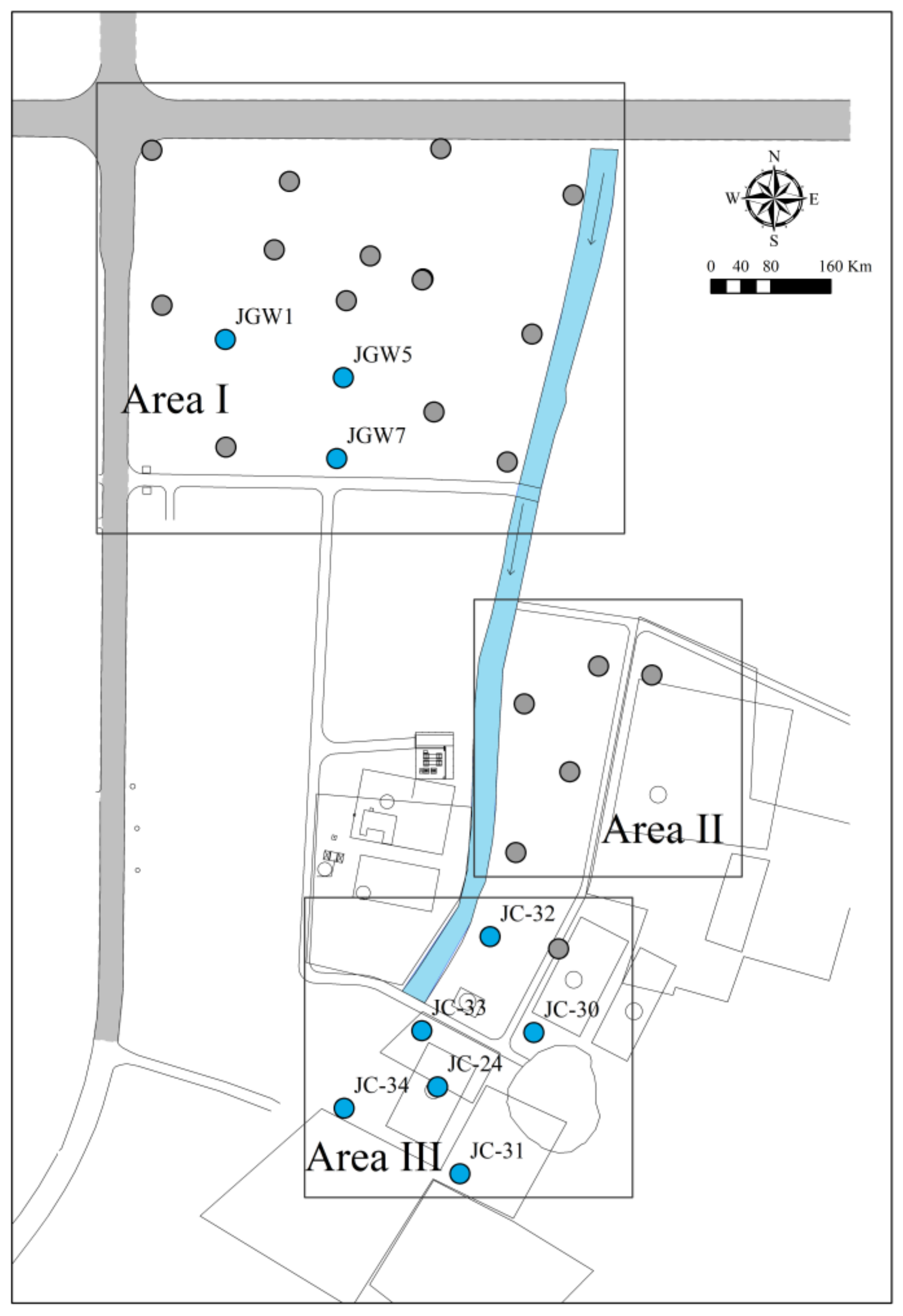
2.1. Study Site
2.2. Sampling Method
2.3. Laboratory Analysis
2.4. Prediction Model
2.4.1. Variables’ Selection
2.4.2. Data Processing Method
2.4.3. Model Description
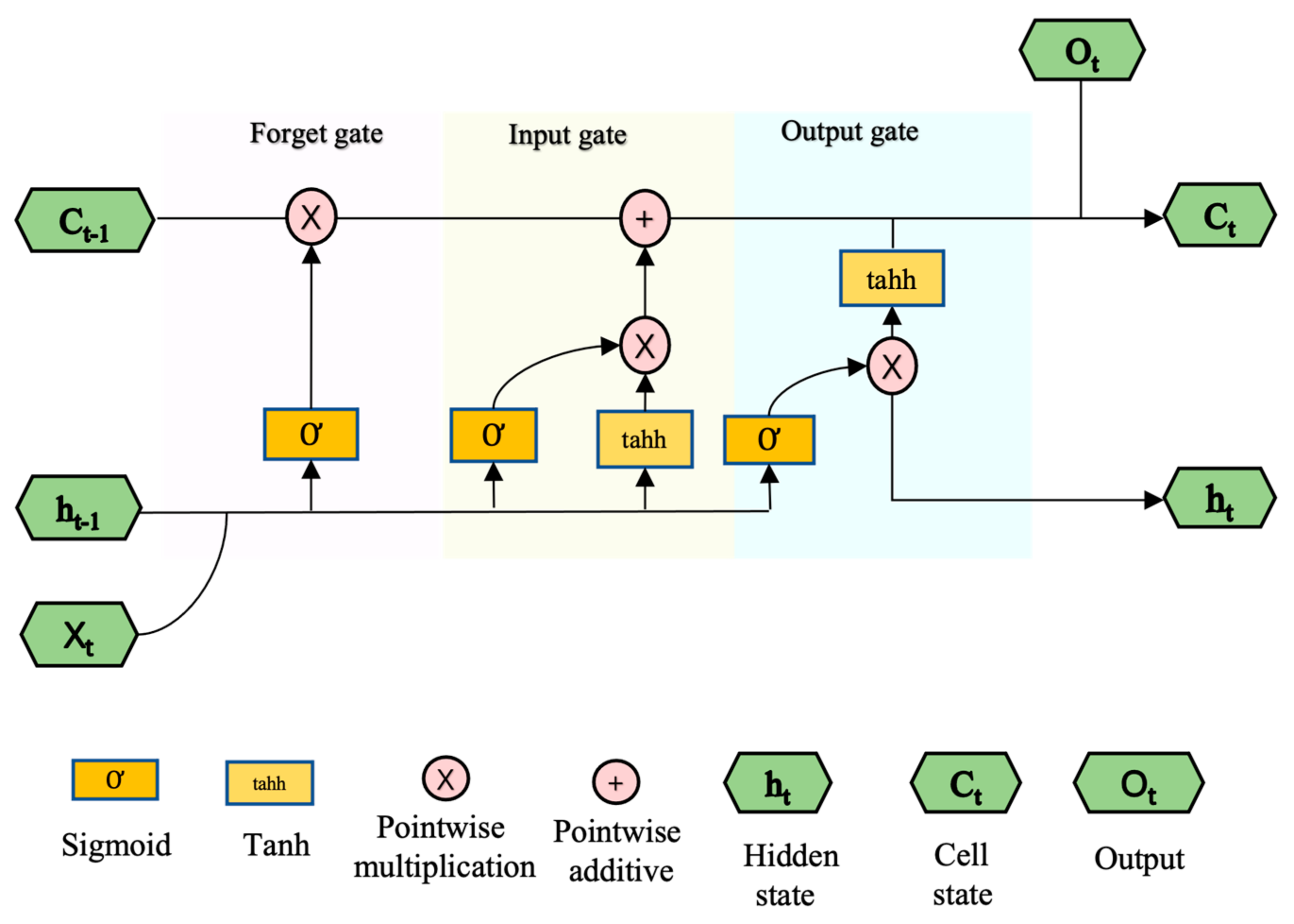
Long Short-Term Memory (LSTM)
Extreme Gradient Boosting (XGBoost)
SHapley Additive exPlanations (SHAP)
2.4.4. Model Training and Evaluation
Model Training
Model Evaluation
3. Results
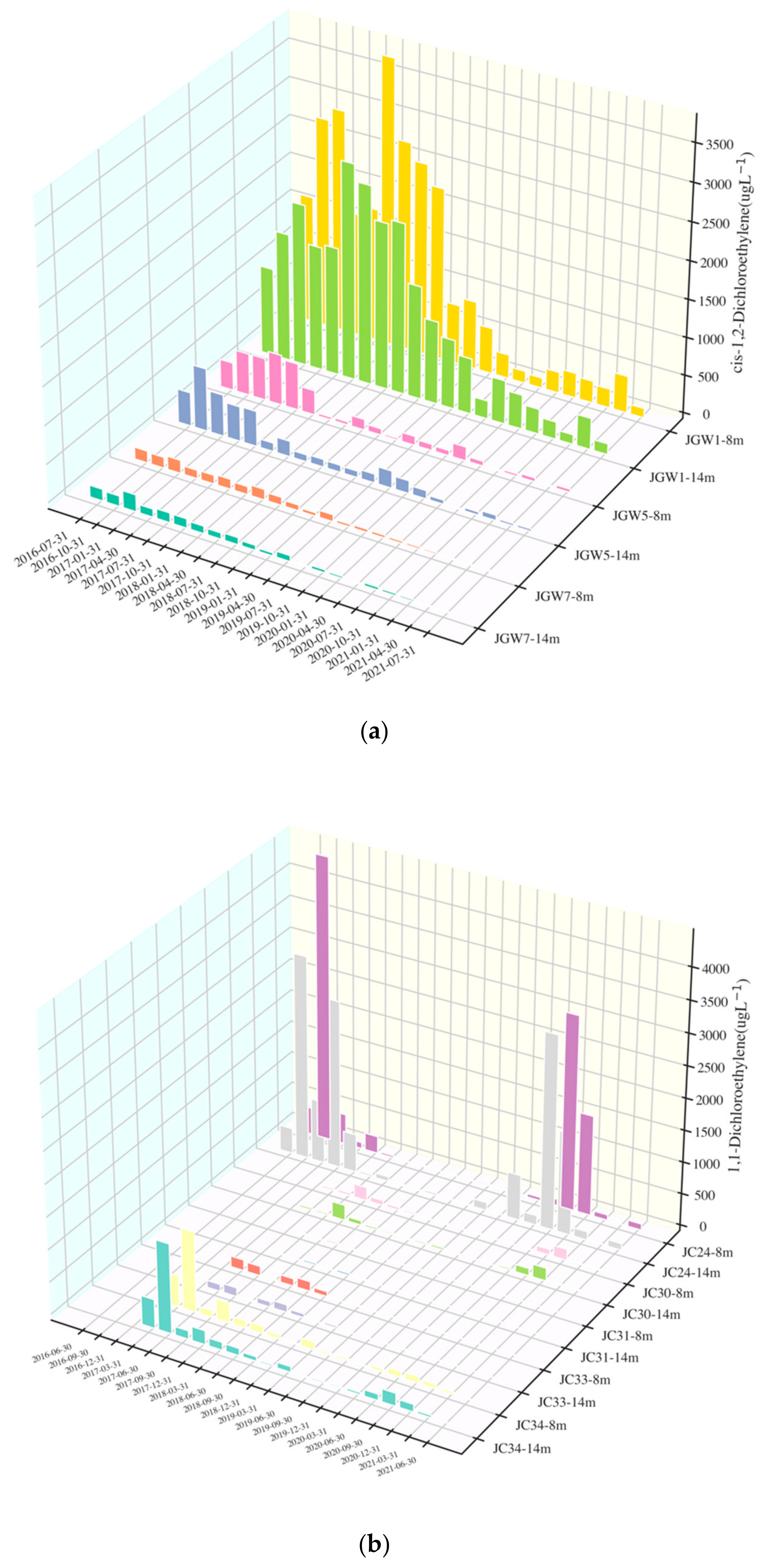
3.1. Characteristics of Selected Wells
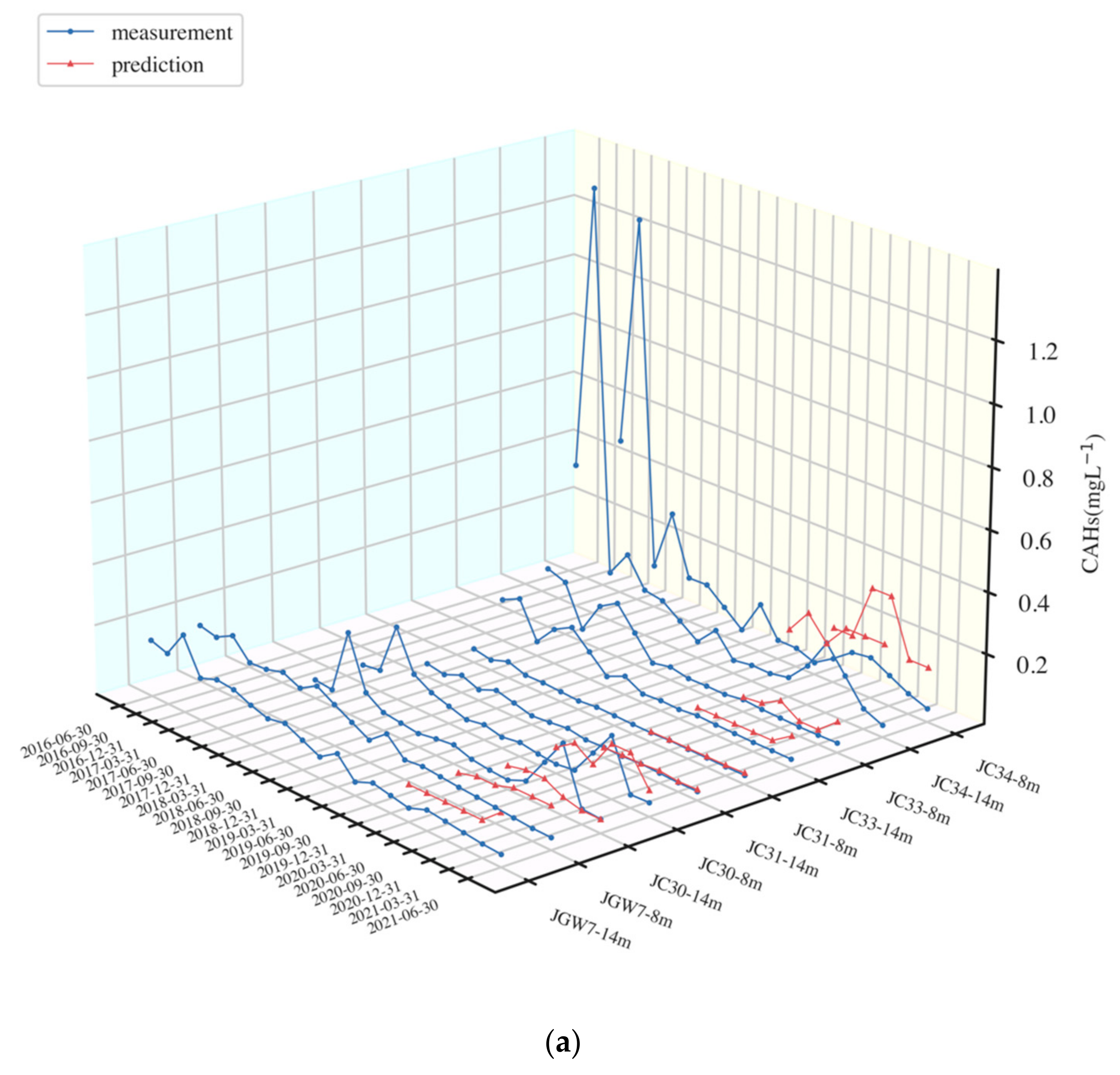
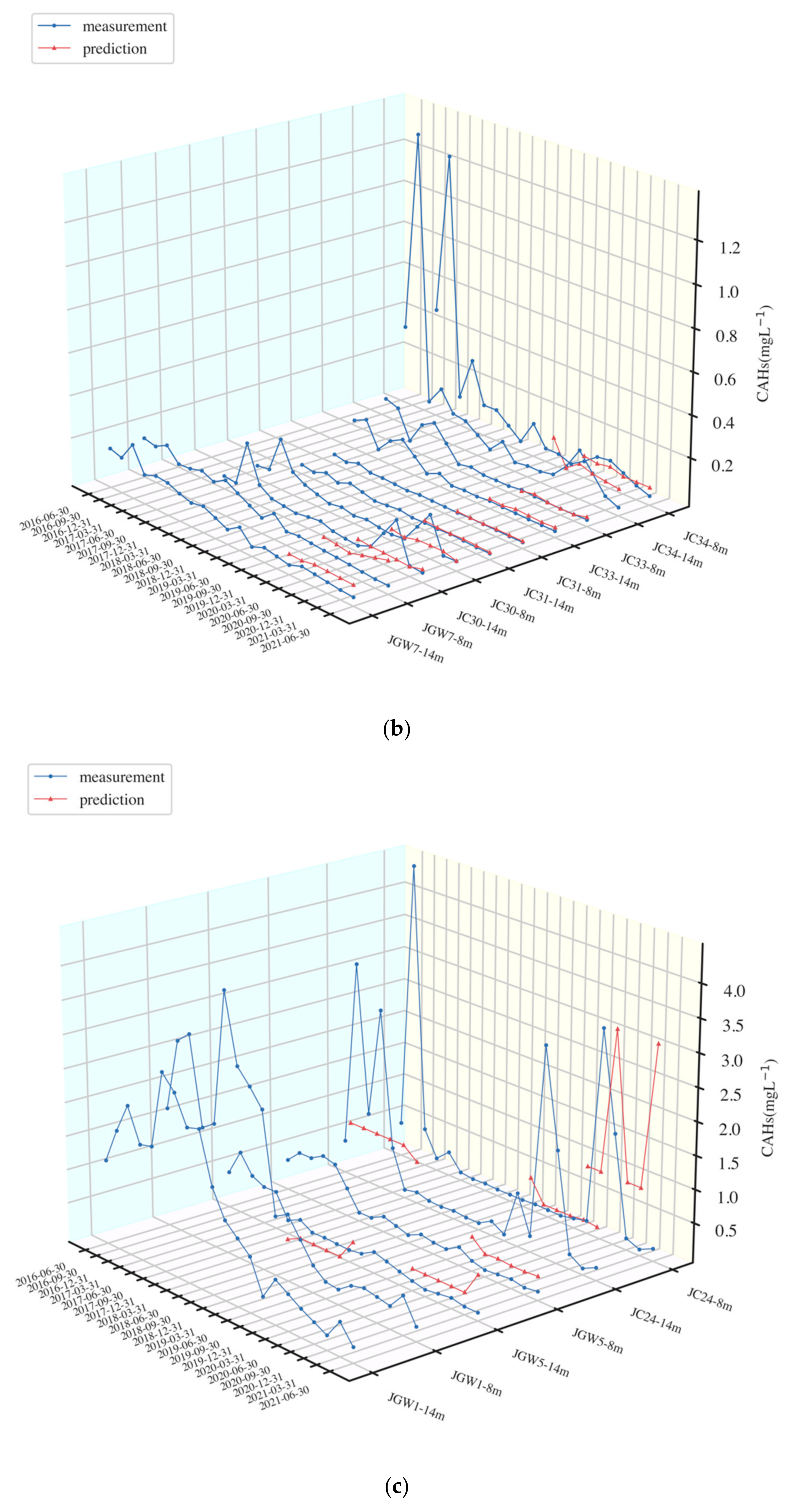
3.2. Prediction Results of XGBoost and LSTM
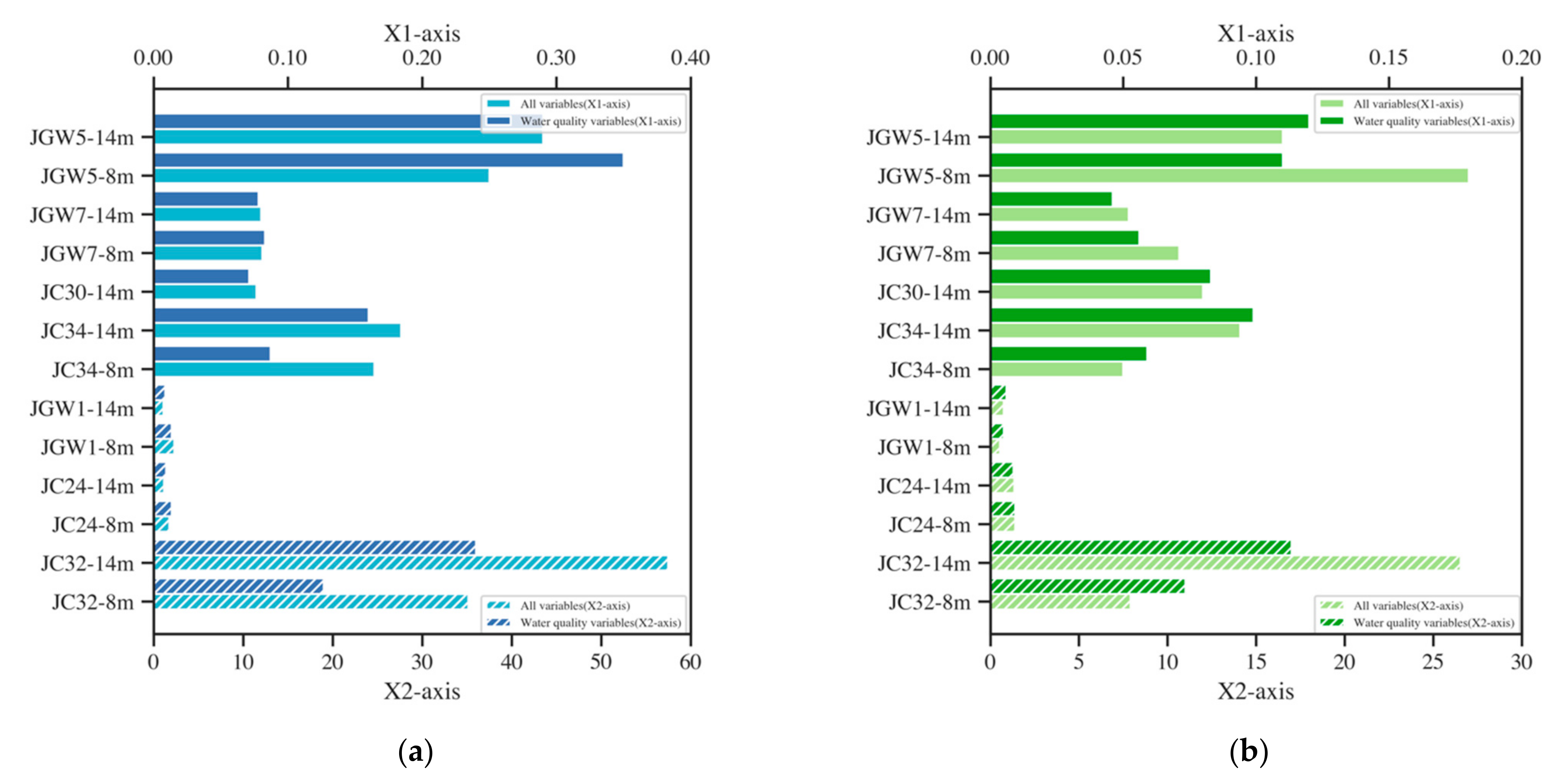
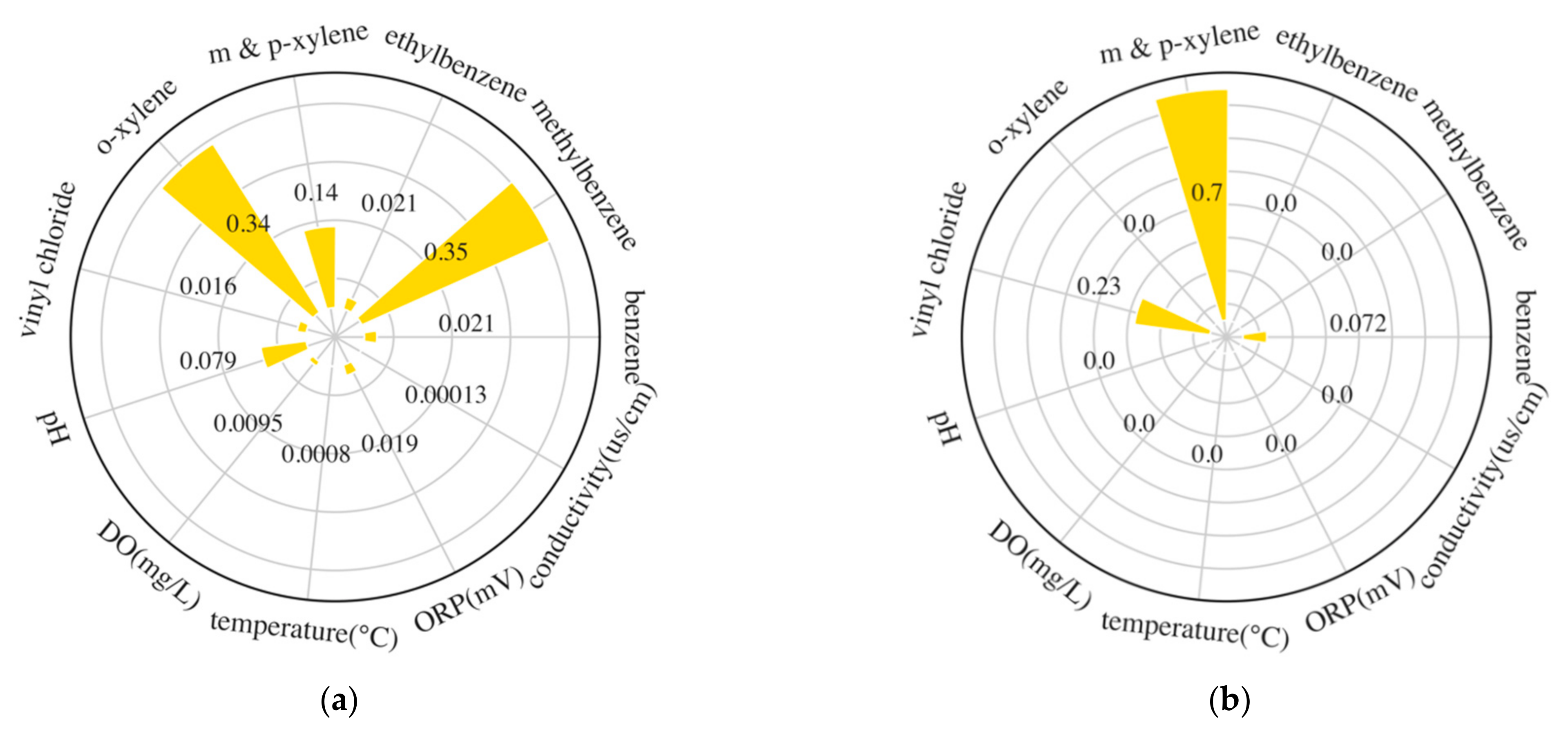
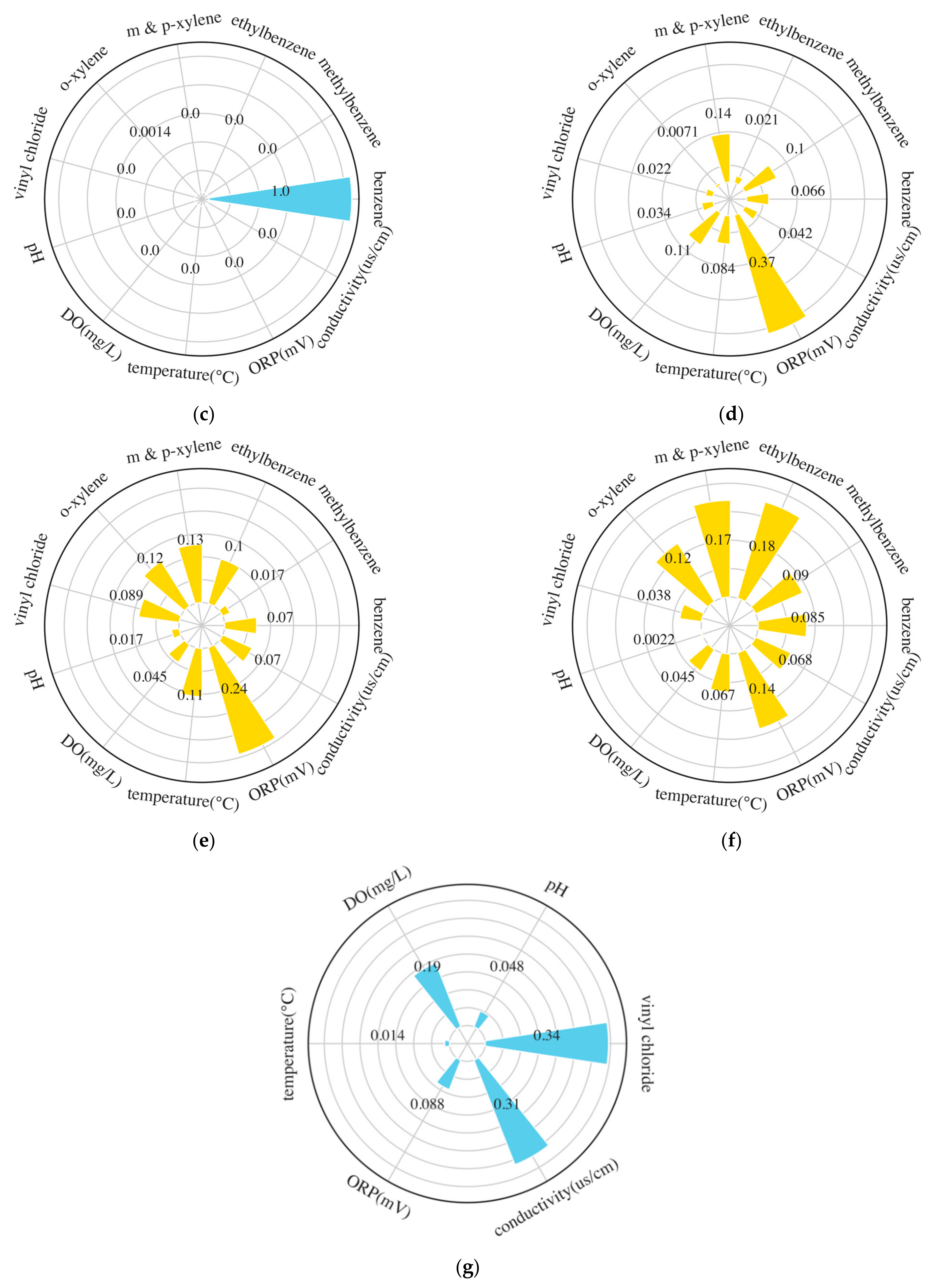
3.3. SHAP Analysis on XGBoost and LSTM
3.4. Prediction Results of Water Quality Indicators
4. Discussion
4.1. Influences on Models’ Prediction
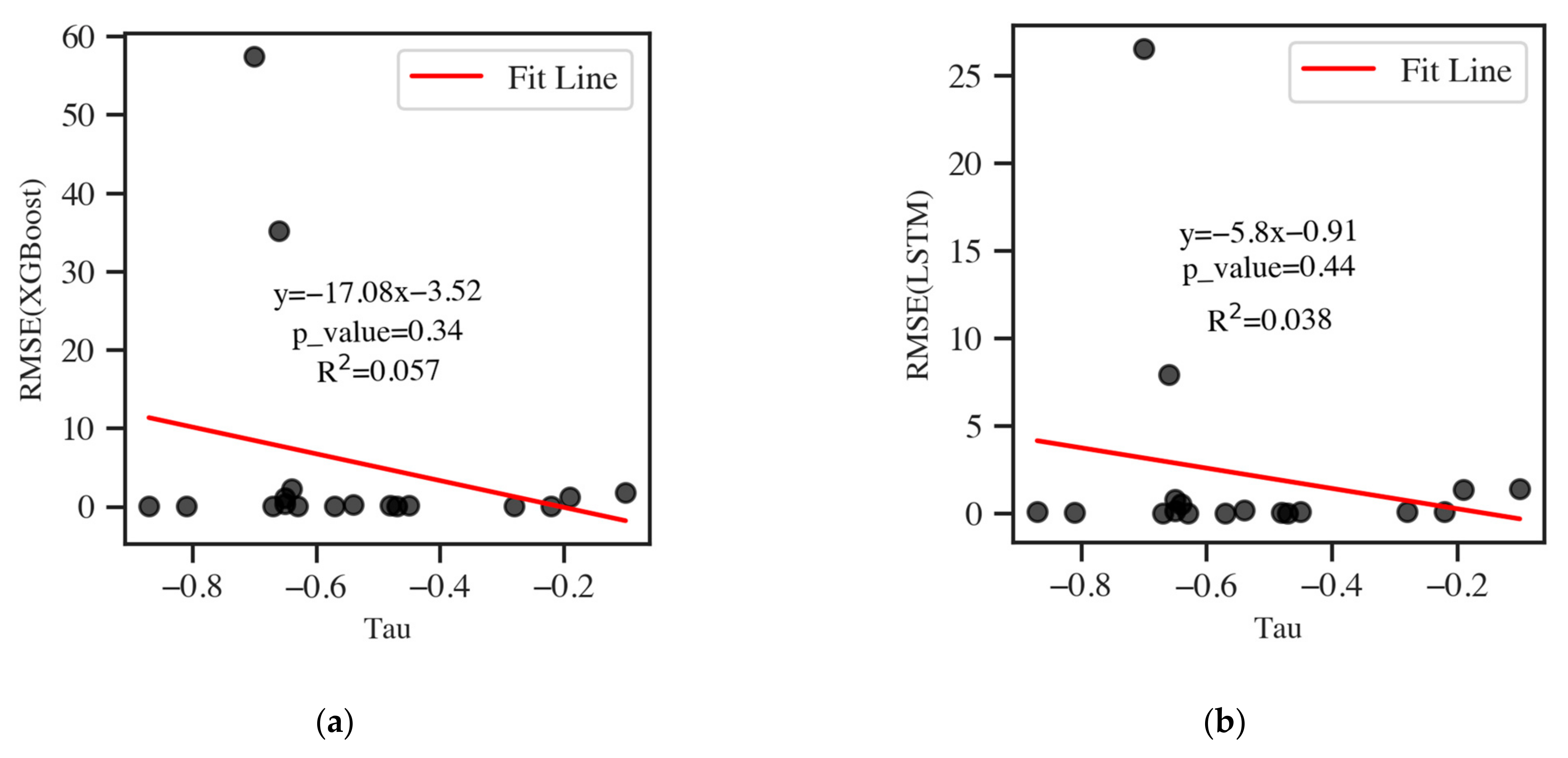
4.1.1. Influences of DCE Concentrations
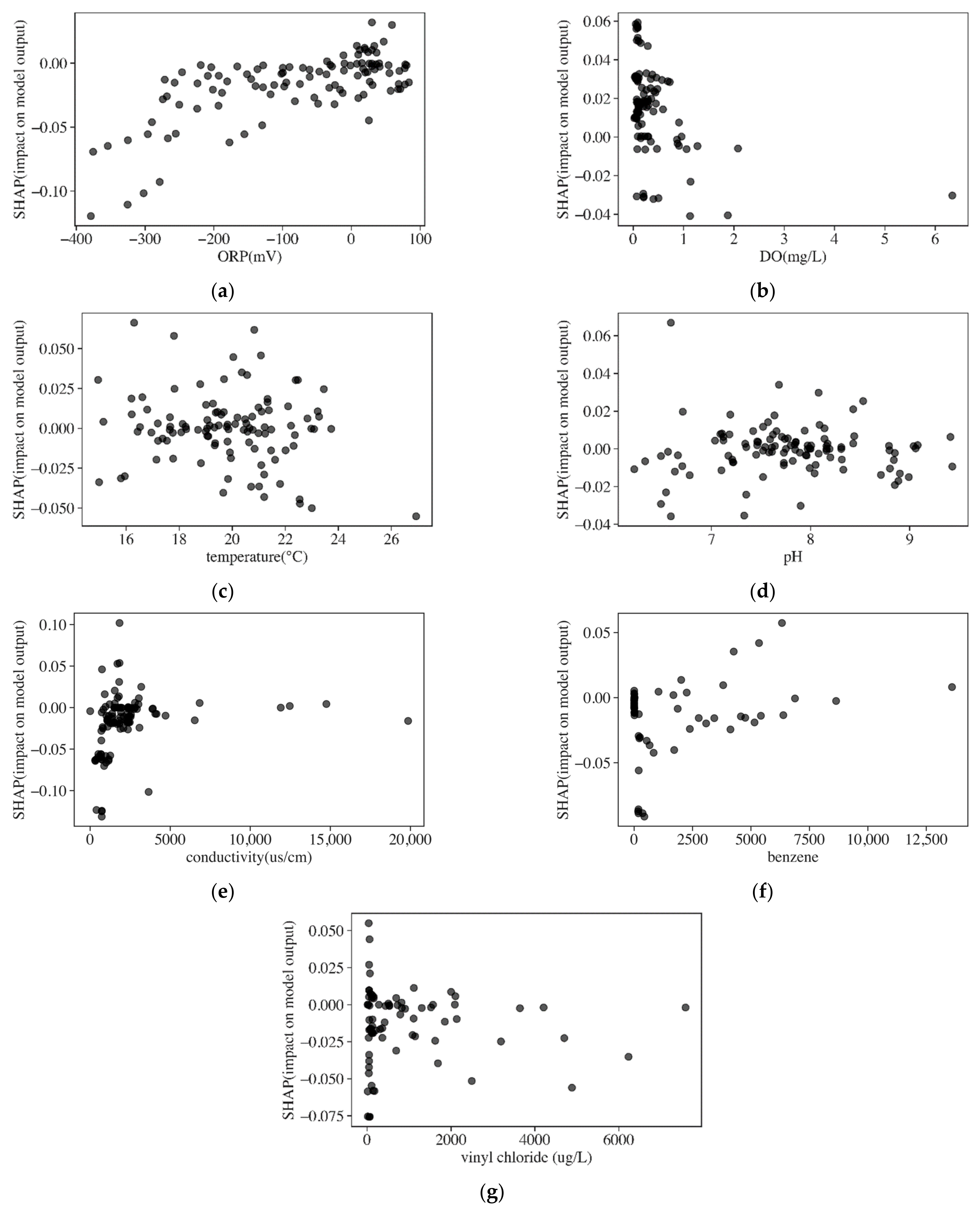
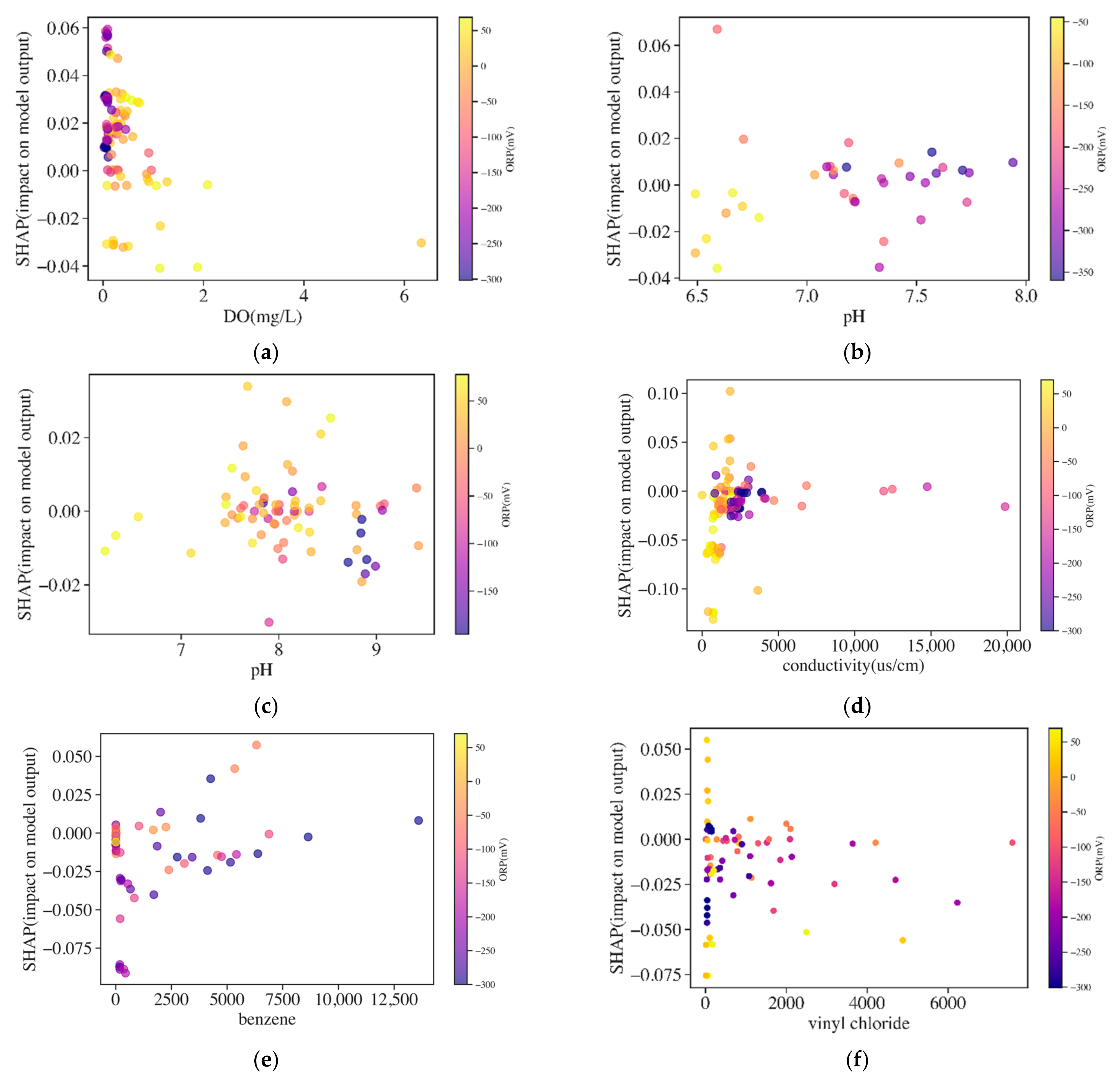
4.1.2. Influences of Variables
Water Quality Indicators
Organic Indicators
4.2. Comparison between XGBoost and LSTM
4.3. Suggestions for the Model and the Potential for Low-Cost Modeling
5. Conclusions
Supplementary Materials
Author Contributions
Funding
Institutional Review Board Statement
Informed Consent Statement
Data Availability Statement
Conflicts of Interest
References
- Lien, P.J.; Yang, Z.H.; Chang, Y.M.; Tu, Y.T.; Kao, C.M. Enhanced bioremediation of TCE-contaminated groundwater with coexistence of fuel oil: Effectiveness and mechanism study. Chem. Eng. J. 2016, 289, 525–536. [Google Scholar] [CrossRef]
- Danish, M.; Gu, X.; Lu, S.; Farooq, U.; Ahmad, A.; Naqvi, M.; Zhang, X.; Fu, X.; Xue, Y. Effect of solution matrix and pH in Z-nZVI-catalyzed percarbonate system on the generation of reactive oxygen species and degradation of 1,1,1-trichloroethane. Water Supply 2017, 6, 1568–1578. [Google Scholar] [CrossRef]
- Lu, Q.; Luo, Q.; Li, H.; Liu, Y.; Gu, J.; Lin, K. Characterization of chlorinated aliphatic hydrocarbons and environmental variables in a shallow groundwater in Shanghai using kriging interpolation and multifactorial analysis. PLoS ONE 2015, 10, e0142241. [Google Scholar] [CrossRef] [Green Version]
- Ko, J.; Musson, S.; Townsend, T. Removal of trichloroethylene from soil using the hydration of calcium oxide. J. Environ. Manag. 2011, 92, 1767–1773. [Google Scholar] [CrossRef] [PubMed]
- Wright, J.; Kirchner, V.; Bernard, W.; Ulrich, N.; McLimans, C.; Campa, M.; Hazen, T.; Macbeth, T.; Marabello, D.; McDermott, J.; et al. Bacterial community dynamics in dichloromethane-contaminated groundwater undergoing natural attenuation. Front. Microbiol. 2017, 22, 2300. [Google Scholar] [CrossRef]
- Rahim, F.; Abdullah, S.; Hasan, H.; Kurniawan, S.; Mamat, A.; Yusof, K.; Ambak, K. A feasibility study for the treatment of 1,2-dichloroethane-contaminated groundwater using reedbed system and assessment of its natural attenuation. Sci. Total Environ. 2022, 814, 152799. [Google Scholar] [CrossRef]
- Scheutz, C.; Durant, N.; Hansen, M.; Bjerg, P. Natural and enhanced anaerobic degradation of 1,1,1-trichloroethane and its degradation products in the subsurface—A critical review. Water Res. 2011, 45, 2701–2723. [Google Scholar] [CrossRef] [PubMed]
- Wiedemeier, T.; Swanson, M.; Moutoux, D.; Kinzie Gordon, E.; Wilson, B.; Kampbell, D.; Haas, P.; Miller, R.; Hansen, J.; Chapelle, F.; et al. Technical Protocol for Evaluating Natural Attenuation of Chlorinated Solvents in Groundwater; EPA/600/R-98/128; Office of Research and Development, U.S. EPA: Washington, DC, USA, 1998. Available online: https://semspub.epa.gov/work/06/668746.pdf (accessed on 20 March 2022).
- Broholm, K.; Ludvigsen, L.; Jensen, T.; Østergaard, H. Aerobic biodegradation of vinyl chloride and cis-1,2-dichloroethene in aquifer sediments. Chemosphere 2005, 60, 1555–1564. [Google Scholar] [CrossRef]
- Freedman, D.; Gossett, J. Biological reductive dechlorination of tetrachloroethylene and trichloroethylene to ethylene under methanogenic conditions. Appl. Environ. Microbiol. 1989, 55, 2144–2151. [Google Scholar] [CrossRef] [Green Version]
- Yang, J.; Zhang, Q.; Fu, X.; Chen, H.; Hu, P.; Wang, L. Natural attenuation mechanism and health risk assessment of 1,1,2-trichloroethane in contaminated groundwater. J. Environ. Manag. 2019, 242, 457–464. [Google Scholar] [CrossRef]
- Zhong, S.; Zhang, K.; Bagheri, M.; Burken, J.; Gu, A.; Li, B.; Ma, X.; Marrone, B.L.; Ren, Z.J.; Schrier, J.; et al. Machine Learning: New Ideas and Tools in Environmental Science and Engineering. Environ. Sci. Technol. 2021, 55, 12741–12754. [Google Scholar] [CrossRef] [PubMed]
- Le, X.; Ho, H.; Lee, G.; Jung, S. Application of Long Short-Term Memory (LSTM) neural network for flood forecasting. Water 2019, 11, 1387. [Google Scholar] [CrossRef] [Green Version]
- Vu, M.; Jardani, A.; Massei, N.; Fournier, M. Reconstruction of missing groundwater level data by using Long Short-Term Memory (LSTM) deep neural network. J. Hydrol. 2021, 597, 125776. [Google Scholar] [CrossRef]
- Zhi, W.; Feng, D.; Tsai, W.; Sterle, G.; Harpold, A.; Shen, C.; Li, L. From Hydrometeorology to River Water Quality: Can a Deep Learning Model Predict Dissolved Oxygen at the Continental Scale? Environ. Sci. Technol. 2021, 55, 2357–2368. [Google Scholar] [CrossRef] [PubMed]
- Feng, D.; Fang, K.; Shen, C. Enhancing streamflow forecast and extracting insights using long-short term memory networks with data integration at continental scales. Water Resour. Res. 2020, 56, e2019WR026793. [Google Scholar] [CrossRef]
- Hu, Z.; Zhang, Y.; Zhao, Y.; Xie, M.; Zhong, J.; Tu, Z.; Liu, J. A water quality prediction method based on the deep LSTM network considering correlation in smart mariculture. Sensors 2019, 6, 1420. [Google Scholar] [CrossRef] [PubMed] [Green Version]
- Ching, P.; Zou, X.; Wu, D.; So, R.; Chen, G. Development of a wide-range soft sensor for predicting wastewater BOD5 using an eXtreme gradient boosting (XGBoost) machine. Environ. Res. 2022, 210, 112953. [Google Scholar] [CrossRef]
- Sharafati, A.; Asadollah, S.; Hosseinzadeh, M. The potential of new ensemble machine learning models for effluent quality parameters prediction and related uncertainty. Proc. Saf. Environ. 2020, 140, 68–78. [Google Scholar] [CrossRef]
- Chen, T.; Guestrin, C. XGBoost: A scalable tree boosting system. In Proceedings of the 22nd ACM SIGKDD International Conference on Knowledge Discovery and Data Mining (KDD ’16), San Francisco, CA, USA, 13–17 August 2016; pp. 784–794. [Google Scholar]
- Lundberg, S.; Lee, S. A unified approach to interpreting model predictions. In Proceedings of the 31st International Conference on Neural Information Processing Systems (NIPS’17), Long Beach, CA, USA, 4–9 December 2016; Curran Associates Inc.: Red Hook, NY, USA, 2017; pp. 4768–4777. [Google Scholar]
- Lundberg, S.; Erion, G.; Lee, S. Consistent Individualized Feature Attribution for Tree Ensembles. arXiv 2018, arXiv:1802.03888. [Google Scholar]
- Hochreiter, S.; Schmidhuber, J. Long short-term memory. Neural Comput. 1997, 9, 1735–1780. [Google Scholar] [CrossRef]
- Man, Y.; Yang, Q.; Shao, J.; Wang, G.; Bai, L.; Xue, Y. Enhanced LSTM model for daily runoff prediction in the upper Huai river basin, China. Engineering, 2022; in press. [Google Scholar] [CrossRef]
- Engelmann, C.; Händel, F.; Binder, M.; Yadav, P.; Dietrich, P.; Liedl, R.; Walther, M. The fate of DNAPL contaminants in non-consolidated subsurface systems—Discussion on the relevance of effective source zone geometries for plume propagation. J. Hazard. Mater. 2019, 375, 233–240. [Google Scholar] [CrossRef] [PubMed]
- Cavelan, A.; Golfier, F.; Colombano, S.; Davarzani, H.; Deparis, J.; Faure, P. A critical review of the influence of groundwater level fluctuations and temperature on LNAPL contaminations in the context of climate change. Sci. Total Environ. 2022, 806, 150412. [Google Scholar] [CrossRef] [PubMed]
- Flores, G.; Katsumi, T.; Inui, T.; Kamon, M. A simplified image analysis method to study lnapl migration in porous media. Soils Found. 2011, 51, 835–847. [Google Scholar] [CrossRef] [Green Version]
- Wang, D.; Thunell, S.; Lindberg, U.; Jiang, L.; Trygg, J.; Tysklind, M. Towards better process management in wastewater treatment plants: Process analytics based on SHAP values for tree-based machine learning methods. J. Environ. Manag. 2022, 301, 113941. [Google Scholar] [CrossRef] [PubMed]
- Cerna, S.; Guyeux, C.; Arcolezi, H.; Couturier, R.; Royer, G. A Comparison of LSTM and XGBoost for Predicting Firemen Interventions. Available online: https://hharcolezi.github.io/files/2019_WCIST_LSTM_vs_XGBoost.pdf (accessed on 20 April 2022).
- Jiang, Y.; Li, C.; Song, H.; Wang, W. Deep learning model based on urban multi-source data for predicting heavy metals (Cu, Zn, Ni, Cr) in industrial sewer networks. J. Hazard. Mater. 2022, 432, 128732. [Google Scholar] [CrossRef]
- Mortan, S.; Martín-González, L.; Vicent, T.; Caminal, G.; Nijenhuis, I.; Adrian, L.; Marco-Urrea, E. Detoxification of 1,1,2-trichloroethane to ethene in a bioreactor co-culture of Dehalogenimonas and Dehalococcoides mccartyi strains. J. Hazard. Mater. 2017, 331, 218–225. [Google Scholar] [CrossRef]
- Nemecek, J.; Dolinova, I.; Machackova, J.; Spanek, R.; Sevcu, A.; Lederer, T.; Cernik, M. Stratification of chlorinated ethenes natural attenuation in an alluvial aquifer assessed by hydrochemical and biomolecular tools. Chemosphere 2017, 184, 1157–1167. [Google Scholar] [CrossRef]
- Chang, C.; Yang, H.; Hung, J.; Lu, C.; Liu, M. Simulation of combined anaerobic/aerobic bioremediation of tetrachloroethylene in groundwater by a column system. Int. Biodeter. Biodegr. 2017, 117, 150–157. [Google Scholar] [CrossRef]
- Wu, N.; Zhang, W.; Wei, W.; Yang, S.; Wang, H.; Sun, Z.; Song, Y.; Li, P.; Yang, Y. Field study of chlorinated aliphatic hydrocarbon degradation in contaminated groundwater via micron zero-valent iron coupled with biostimulation. Chem. Eng. J. 2019, 284, 123349. [Google Scholar] [CrossRef]
- Zhang, X.; Luo, M.; Deng, S.; Long, T.; Sun, L.; Yu, R. Field study of microbial community structure and dechlorination activity in a multi-solvents co-contaminated site undergoing natural attenuation. J. Hazard. Mater. 2022, 423 Pt A, 127010. [Google Scholar] [CrossRef]
- Cubillos, M. Multi-site household waste generation forecasting using a deep learning approach. Waste Manag. 2020, 115, 8–14. [Google Scholar] [CrossRef] [PubMed]


| Well | Indicator | Tau | p-Value | Std | Mean | Range |
|---|---|---|---|---|---|---|
| JGW7-14m | cis-1,2-DCE | −0.81 | 3.21 × 10⁻⁹ | 56.11 | 75.08 | 12.7–225 |
| JGW7-8m | cis-1,2-DCE | −0.87 | 3.23 × 10⁻⁸ | 52.45 | 78.16 | 11.6–175 |
| JGW5-14m | cis-1,2-DCE | −0.65 | 1.13 × 10⁻⁵ | 210.84 | 204.75 | 13.4–826 |
| JGW5-8m | cis-1,2-DCE | −0.54 | 3.63 × 10⁻⁴ | 215.58 | 194.27 | 13.2–664 |
| JGW1-14m | cis-1,2-DCE | −0.65 | 3.49 × 10⁻⁵ | 849.37 | 1185.95 | 127–2840 |
| JGW1-8m | cis-1,2-DCE | −0.64 | 1.62 × 10⁻⁵ | 1125.59 | 1273.33 | 127–3780 |
| JC24-14m | 1,1-DCE | −0.19 | 2.39 × 10⁻¹ | 1021.69 | 662.29 | 5.6–3205 |
| JC24-8m | 1,1-DCE | −0.10 | 5.71 × 10⁻¹ | 1128.40 | 516.47 | 3–4470 |
| JC30-14m | 1,1-DCE | −0.22 | 2.36 × 10⁻¹ | 66.45 | 53.03 | 2–240 |
| JC30-8m | 1,1-DCE | −0.28 | 1.29 × 10⁻¹ | 58.51 | 48.30 | 1.7–211 |
| JC31-14m | 1,1-DCE | −0.47 | 1.15 × 10⁻² | 9.29 | 9.45 | 0.7–31.8 |
| JC31-8m | 1,1-DCE | −0.63 | 3.36 × 10⁻⁴ | 6.47 | 6.13 | 0.8–26.2 |
| JC32-14m | 1,1-DCE | −0.70 | 1.18 × 10⁻⁵ | 36,457.41 | 27,074.67 | 36.9–115,000 |
| JC32-8m | 1,1-DCE | −0.66 | 4.59 × 10⁻⁵ | 30,503.07 | 20,623.70 | 27.4–105,000 |
| JC33-14m | 1,1-DCE | −0.67 | 1.76 × 10⁻⁴ | 46.37 | 35.59 | 0.9–138.1 |
| JC33-8m | 1,1-DCE | −0.57 | 9.01 × 10⁻⁴ | 60.41 | 43.19 | 2–169 |
| JC34-14m | 1,1-DCE | −0.45 | 8.54 × 10⁻³ | 311.65 | 177.02 | 10.5–1390 |
| JC34-8m | 1,1-DCE | −0.48 | 5.14 × 10⁻³ | 285.68 | 170.98 | 10.8–1250 |
| Well | XGBoost | LSTM | ||||
|---|---|---|---|---|---|---|
| RMSE | MAE | MAPE | RMSE | MAE | MAPE | |
| cis-1,2-DCE | ||||||
| JGW7-14m | 0.08 | 0.076 | 4.30 | 0.052 | 0.050 | 2.80 |
| JGW7-8m | 0.081 | 0.078 | 4.80 | 0.071 | 0.069 | 4.20 |
| JGW5-14m | 0.29 | 0.25 | 8.60 | 0.11 | 0.096 | 3.80 |
| JGW5-8m | 0.25 | 0.25 | 9.50 | 0.18 | 0.14 | 5.00 |
| JGW1-14m | 1.10 | 1.10 | 5.30 | 0.76 | 0.67 | 3.60 |
| JGW1-8m | 2.30 | 2.30 | 9.30 | 0.53 | 0.44 | 2.20 |
| Average | 0.68 | 0.68 | 6.97 | 0.28 | 0.24 | 3.60 |
| 1,1-DCE | ||||||
| JC24-14m | 1.17 | 1.0010 | 24.40 | 1.35 | 0.77 | 3.91 |
| JC24-8m | 1.75 | 1.548 | 59.76 | 1.40 | 0.82 | 0.82 |
| JC30-14m | 0.077 | 0.052 | 4.26 | 0.080 | 0.055 | 4.03 |
| JC30-8m | 0.073 | 0.063 | 8.75 | 0.068 | 0.042 | 2.24 |
| JC31-14m | 0.0044 | 0.0036 | 2.49 | 0.0049 | 0.0045 | 2.72 |
| JC31-8m | 0.0043 | 0.0040 | 2.83 | 0.0037 | 0.0032 | 2.26 |
| JC32-14m | 57.46 | 54.68 | 563.40 | 26.54 | 21.07 | 253.60 |
| JC32-8m | 35.16 | 34.45 | 415.80 | 7.90 | 7.31 | 103.70 |
| JC33-14m | 0.041 | 0.038 | 17.62 | 0.013 | 0.011 | 5.37 |
| JC33-8m | 0.039 | 0.032 | 9.02 | 0.0074 | 0.0067 | 1.74 |
| JC34-14m | 0.18 | 0.16 | 6.46 | 0.094 | 0.076 | 2.97 |
| JC34-8m | 0.16 | 0.15 | 3.30 | 0.050 | 0.044 | 1.19 |
| Average | 8.01 | 7.68 | 93.18 | 3.13 | 2.52 | 32.05 |
Publisher’s Note: MDPI stays neutral with regard to jurisdictional claims in published maps and institutional affiliations. |
© 2022 by the authors. Licensee MDPI, Basel, Switzerland. This article is an open access article distributed under the terms and conditions of the Creative Commons Attribution (CC BY) license (https://creativecommons.org/licenses/by/4.0/).
Share and Cite
Xia, F.; Jiang, D.; Kong, L.; Zhou, Y.; Wei, J.; Ding, D.; Chen, Y.; Wang, G.; Deng, S. Prediction of Dichloroethene Concentration in the Groundwater of a Contaminated Site Using XGBoost and LSTM. Int. J. Environ. Res. Public Health 2022, 19, 9374. https://doi.org/10.3390/ijerph19159374
Xia F, Jiang D, Kong L, Zhou Y, Wei J, Ding D, Chen Y, Wang G, Deng S. Prediction of Dichloroethene Concentration in the Groundwater of a Contaminated Site Using XGBoost and LSTM. International Journal of Environmental Research and Public Health. 2022; 19(15):9374. https://doi.org/10.3390/ijerph19159374
Chicago/Turabian StyleXia, Feiyang, Dengdeng Jiang, Lingya Kong, Yan Zhou, Jing Wei, Da Ding, Yun Chen, Guoqing Wang, and Shaopo Deng. 2022. "Prediction of Dichloroethene Concentration in the Groundwater of a Contaminated Site Using XGBoost and LSTM" International Journal of Environmental Research and Public Health 19, no. 15: 9374. https://doi.org/10.3390/ijerph19159374
APA StyleXia, F., Jiang, D., Kong, L., Zhou, Y., Wei, J., Ding, D., Chen, Y., Wang, G., & Deng, S. (2022). Prediction of Dichloroethene Concentration in the Groundwater of a Contaminated Site Using XGBoost and LSTM. International Journal of Environmental Research and Public Health, 19(15), 9374. https://doi.org/10.3390/ijerph19159374