
Socioeconomic and Demographic Factors Effect in Association with Driver’s Medical Services after Crashes

 ,
,  ,
,
Abstract
:1. Introduction
2. Materials and Methods
2.1. Dataset Development
2.2. Socioeconomic Data
2.3. Statistical Analysis
2.4. Model Development Process
3. Results
3.1. Correlation Test
3.2. Recursive Partitioning Analysis
3.3. Final Model
4. Discussion
5. Conclusions
Author Contributions
Funding
Conflicts of Interest
Appendix A

| Category | Variable | Category | Variable |
|---|---|---|---|
| Race | Percent white (WH) | Marital Status | Percent now married (MRD) |
| Percent black (BL) | Percent widowed (WID) | ||
| Percent American Indian (AI) | Percent divorced (DIV) | ||
| Percent Asian (AS) | Percent separated (SEP) | ||
| Percent other races (OR) | Percent never married (NMD) | ||
| Housing | Household units (HH) | Education | Percent less than high school graduate (LHS) |
| Household ownership total (HHO) | Percent high school graduate (HS) | ||
| Owner occupied housing units (OHU) | Percent some college/associate degree (COL) | ||
| Renter occupied housing units (RHU) | Percent bachelor’s degree or higher (BS) | ||
| Median housing value (HVL) | Percent graduate or professional degree (GD) | ||
| Other | Employment population ratio (EMP) | Income | Median individual income (MDIINC) |
| Percentage rural (RUR) | Household median income (MDHINC) | ||
| Unemployment rate (UEMP) | Household mean income (MHINC) | ||
| Percent below poverty level (POV) | Mean individual income (MIINC) | ||
| Total population (POP) | |||
| Variables | Kentucky | Utah | Ohio | |||
|---|---|---|---|---|---|---|
| Relative | Importance | Relative | Importance | Relative | Importance | |
| Percent bachelor’s degree or higher (BS) | 1.000 | 33.969 | 0.543 | 9.292 | 0.667 | 22.4812 |
| Gender | 0.599 | 20.353 | 0.918 | 15.699 | 1.000 | 33.693 |
| Median housing value (HVL) | 0.558 | 18.944 | 0.356 | 12.005 | ||
| Percent graduate or professional degree (GD) | 0.532 | 18.069 | 0.134 | 4.527 | ||
| Age Groups (AGE) | 0.417 | 14.155 | 0.334 | 5.713 | 0.495 | 16.689 |
| Percentage rural (RUR) | 0.396 | 13.465 | 1.000 | 17.108 | 0.216 | 7.292 |
| Employment population ratio (EMP) | 0.335 | 11.364 | 0.267 | 4.497 | ||
| Percent white (WH) | 0.230 | 7.817 | 0.083 | 1.412 | ||
| Percent high school graduate (HS) | 0.206 | 7.005 | 0.178 | 3.046 | 0.186 | 6.275 |
| Percent less than high school graduate (LHS) | 0.194 | 6.587 | 0.553 | 9.454 | ||
| Percent some college/associate degree (COL) | 0.193 | 6.553 | 0.188 | 3.209 | 0.264 | 8.883 |
| Percent black (BL) | 0.247 | 4.229 | 0.188 | 6.321 | ||
| State | Variables | Linked | Unlinked | ||||||||
|---|---|---|---|---|---|---|---|---|---|---|---|
| N | Minimum | Maximum | Mean | Std. Deviation | N | Minimum | Maximum | Mean | Std. Deviation | ||
| Kentucky | RUR 1 | 114,051 | 0 | 10 | 4.45 | 3.80 | 114,051 | 0 | 10 | 3.73 | 3.66 |
| EMP 1 | 114,046 | 0 | 10 | 5.37 | 1.01 | 114,043 | 0 | 10 | 5.59 | 0.95 | |
| BS 1 | 114,046 | 0 | 5.13 | 1.13 | 0.68 | 114,043 | 0 | 5.13 | 1.31 | 0.76 | |
| HVL 2 | 113,363 | 2.14 | 38.53 | 12.22 | 4.90 | 113,484 | 2.14 | 38.53 | 13.44 | 5.42 | |
| Utah | RUR 1 | 65,316 | 0.87 | 10 | 1.03 | 1.71 | 65,316 | 0.87 | 10 | 0.87 | 1.59 |
| EMP 1 | 64,669 | 11.8 | 8.48 | 6.54 | 0.58 | 64,577 | 0 | 10.00 | 6.59 | 0.53 | |
| BS 1 | 64,669 | 0 | 5.353 | 1.84 | 0.67 | 64,577 | 0 | 6.41 | 1.92 | 0.69 | |
| HVL 2 | 113,363 | 2.91 | 101.5 | 25.59 | 8.48 | 113,484 | 2.91 | 101.5 | 26.60 | 9.09 | |
| Ohio | RUR 1 | 116,098 | 0 | 10 | 7.19 | 3.48 | 131,772 | 0 | 10 | 7.21 | 3.45 |
| EMP 1 | NA | NA | NA | NA | NA | NA | NA | NA | NA | NA | |
| BS 1 | 116,073 | 0 | 5.33 | 1.47 | 0.79 | 131,772 | 0 | 5.33 | 1.58 | 0.88 | |
| HVL 2 | 113,363 | 1.48 | 49.67 | 12.78 | 4.79 | 113,484 | 1.48 | 49.67 | 13.46 | 5.26 | |
References
- KTC. Traffic Collision Facts 2002; Kentucky Transportation Center, University of Kentucky: Lexington, Kentucky, 2003; Available online: https://uknowledge.uky.edu/ktc_researchreports/1663/ (accessed on 15 February 2018).
- KTC. Traffic Collision Facts 2017; Kentucky Transportation Center, University of Kentucky: Lexington, Kentucky, 2018; Available online: https://uknowledge.uky.edu/ktc_researchreports/1614/ (accessed on 15 February 2018).
- Hasselberg, M.; Vaeza, M.; Laflamme, L. Socioeconomic aspects of the circumstances and consequences of car crashes among young adults. Soc. Sci. Med. 2005, 60, 287–295. [Google Scholar] [CrossRef] [PubMed]
- Sagar, S.; Stamatiadis, N.; Stromberg, A. Effect of Socioeconomic and Demographic Factors on Crash Occurrence. Transp. Res. Rec. 2021, 2675, 80–91. [Google Scholar] [CrossRef]
- Noland, R.B.; Oh, L. The effect of infrastructure and demographic change on traffic-related fatalities and crashes: A case study of Illinois county-level data. Accid. Anal. Prev. 2004, 36, 525–532. [Google Scholar] [CrossRef]
- Stamatiadis, N.; Puccini, G. Fatal crash rates in the southeastern united states: Why are they higher? Transp. Res. Rec. 1999, 1665, 118–124. [Google Scholar] [CrossRef]
- Adanu, E.K.; Smith, R.; Powell, L.; Jones, S. Multilevel analysis of the role of human factors in regional disparities in crash outcomes. Accid. Anal. Prev. 2017, 109, 10–17. [Google Scholar] [CrossRef] [PubMed]
- Factor, R.; Mahalel, D.; Yair, G. Inter-group differences in road-traffic crash involvement. Accid. Anal. Prev. 2008, 40, 2000–2007. [Google Scholar] [CrossRef] [PubMed]
- Brown, K.T. A Safety Analysis of Spatial Phenomena about the Residences of Drivers Involved in Crashes. Dissertation Presented to the Graduate School of Clemson University. 2016. Available online: https://www.proquest.com/openview/49271f968da309ebf2ed525360873f0f/1?pq-origsite=gscholar&cbl=18750 (accessed on 4 May 2022).
- Lee, J.; Abdel-Aty, M.; Choi, K. Analysis of Residence Characteristics of at-Fault Drivers in Traffic Crashes. Saf. Sci. 2014, 68, 6–13. [Google Scholar] [CrossRef]
- Noland, R.B.; Quddus, M.A. A Spatially Disaggregate Analysis of Road Casualties in England. Accid. Anal. Prev. 2004, 36, 973–984. [Google Scholar] [CrossRef] [PubMed] [Green Version]
- Blincoe, L.; Miller, T.R.; Zaloshnja, E.; Lawrence, B.A. The Economic and Societal Impact of Motor Vehicle Crashes. National Center for Statistics and Analysis, National Highway Traffic Safety Administration. 2015. Available online: https://trid.trb.org/view/1311862 (accessed on 4 May 2022).
- Chen, H.Y.; Ivers, R.Q.; Martiniuk, A.L.C.; Boufous, S.; Senserrick, T.; Woodward, M.; Stevenson, M.; Norto, R. Socioeconomic status and risk of car crash injury, independent of place of residence and driving exposure: Results from the drive study. J. Epidemiol. Community Health 2010, 64, 998–1003. [Google Scholar] [CrossRef] [PubMed]
- Cook, L.J.; Thomas, A.; Olson, C.; Funai, T.; Simmons, T. Crash Outcome Data Evaluation System (Codes): An Examination of Methodologies and Multi-State Traffic Safety Applications. Available online: https://trid.trb.org/view/1367813 (accessed on 8 May 2019).
- Doggett, S.; Ragland, D.; Felschundneff, G. Evaluating Research on Data Linkage to Assess Underreporting of Pedestrian and Bicyclist Injury in Police Crash Data. Available online: https://escholarship.org/uc/item/0jq5h6f5 (accessed on 16 November 2020).
- Singleton, M.; Xiao, Q.; Agent, K.R. Economic Costs of Low Safety Belt Usage in Motor Vehicle Crashes in Kentucky. 2005. Available online: https://uknowledge.uky.edu/ktc_researchreports/181/ (accessed on 4 April 2018).
- Olsen, C.S.; Thomas, A.M.; Cook, L.J. Hospital charges associated with motorcycle crash factors: A quantile regression analysis. Inj. Prev. 2014, 20, 276–280. [Google Scholar] [CrossRef] [PubMed]
- Wachelder, J.J.; van Drunen, I.; Stassen, P.M.; Brouns, S.H.; Lambooij, S.L.; Aarts, M.J.; Haak, H.R. Association of socioeconomic status with outcomes in older adult community-dwelling patients after visiting the emergency department: A retrospective cohort study. BMJ Open 2017, 7, e019318. [Google Scholar] [CrossRef] [PubMed]
- Andrist, E.; Riley, C.L.; Brokamp, C.; Taylor, S.; Beck, A.F. Neighborhood poverty and pediatric intensive care use. Off. J. Am. Acad. Pediatri. 2019, 144, e20190748. [Google Scholar] [CrossRef] [PubMed]
- ACS. United Census Bureau, American Census Survey. Available online: https://www.census.gov/programs-surveys/acs/ (accessed on 28 May 2017).
- Lambert, J.; Gong, L.; Elliott, C.F.; Thompson, K.; Stromberg, A. RFSA: An r package for finding best subsets and interaction. R J. 2018, 10, 295–308. [Google Scholar] [CrossRef] [PubMed] [Green Version]
- Cardet, J.C.; Chang, K.L.; Rooks, B.J.; Carroll, J.K.; Celedón, J.C.; Coyne-Beasley, T.; Cui, J.; Ericson, B.; Forth, V.E.; Fagan, M.; et al. Socioeconomic status associates with worse asthma morbidity among Black and Latinx adults. J. Allergy Clin. Immunol. 2022; online ahead of print. [Google Scholar] [CrossRef]
- Ukert, B.; Esquivel-Pickett, S.; Oza, M.; DeVries, A.; Sylwestrzak, G. Disparities in health care use among low-salary and high-salary employees. Am. J. Manag. Care 2022, 28, e170–e177. [Google Scholar] [CrossRef] [PubMed]
- Wharam, J.F.; Zhang, F.; Landon, B.E.; Soumerai, S.B.; Ross-Degnan, D. Low-socioeconomic-status enrollees in high-deductible plans reduced high-severity emergency care. Health Aff. 2013, 32, 1398–1406. [Google Scholar] [CrossRef] [PubMed]
- Kullgren, J.T.; Galbraith, A.A.; Hinrichsen, V.L.; Miroshnik, I.; Penfold, R.B.; Rosenthal, M.B.; Landon, B.E.; Lieu, T.A. Health care use and decision making among lower-income families in high deductible health plans. Arch. Intern. Med. 2010, 170, 1918–1925. [Google Scholar] [CrossRef] [PubMed] [Green Version]
- Wharam, J.F.; Graves, A.J.; Zhang, F.; Soumerai, S.B.; Ross-Degnan, D.; Landon, B.E. Two-year trends in cancer screening among low socioeconomic status women in an HMO-based high-deductible health plan. J. Gen. Intern. Med. 2012, 27, 1112–1119. [Google Scholar] [CrossRef] [Green Version]
- Marcozzi, A.; Carr, B.; Liferidge, A.; Baehr, N.; Browne, B. Trends in the contribution of emergency departments to the provision of health care in the USA. Int. J. Health Serv. 2018, 48, 267–288. [Google Scholar] [CrossRef]
- Billings, J.; Parikh, N.; Mijanovich, T. Emergency department use in New York City: A substitute for primary care? Issue Brief (Commonw. Fund) 2000, 443, 1–5. [Google Scholar]
- NHTSA. Traffic Safety Facts, National Highway Traffic Safety Administration; U.S. Department of Transportation: Washington, DC, USA, 2018.
| Age Groups | Kentucky | Utah | Ohio | |||
|---|---|---|---|---|---|---|
| Linked | Unlinked | Linked | Unlinked | Linked | Unlinked | |
| <20 | 38,889 | 40,727 | 7831 | 8559 | 36,403 | 36,915 |
| 20–24 | 14,151 | 13,564 | 10,622 | 10,018 (48.4%) | 46,721 | 53,460 |
| 25–39 | 16,845 | 15,557 | 22,530 | 21,856 (49.2%) | 95,573 | 110,788 |
| 40–64 | 35,349 | 33,297 | 19,330 | 20,112 (51.0%) | 127,640 | 125,907 |
| 65–74 | 5586 | 6997 | 3131 | 3063 (49.3%) | 21,134 | 18,666 |
| >75 | 3231 | 3909 | 1872 | 1708 (47.7%) | 12,659 | 11,339 |
| Total | 114,051 | 114,051 | 65,316 | 65,316 | 357,146 | 357,146 |
| Variables | Kentucky | Utah | Ohio | ||||||
|---|---|---|---|---|---|---|---|---|---|
| B | S.E. | Odds | B | S.E. | Odds | B | S.E. | Odds | |
| Ratio | Ratio | Ratio | |||||||
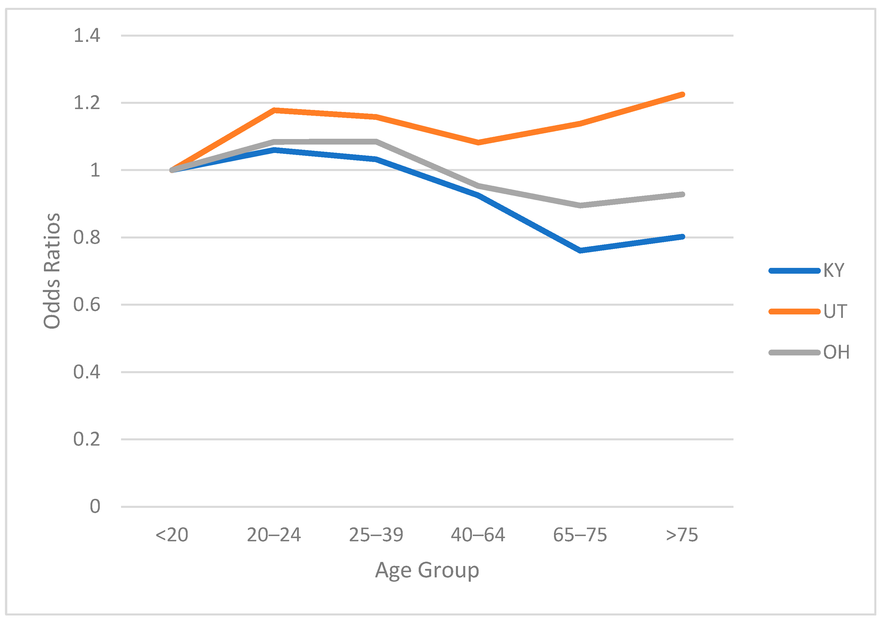
| Age < 20 | ref | 1 | ref | 1 | ref | 1 | |||
| Age 20–24 | 0.059 | 0.017 | 1.06 | 0.164 | 0.021 | 1.178 | 0.08 | 0.01 | 1.084 |
| Age 25–39 | 0.031 | 0.014 | 1.032 | 0.147 | 0.019 | 1.158 | 0.082 | 0.008 | 1.085 |
| Age 40–64 | −0.078 | 0.014 | 0.925 | 0.079 | 0.019 | 1.082 | −0.048 | 0.008 | 0.953 |
| Age 65–75 | −0.273 | 0.022 | 0.761 | 0.129 | 0.03 | 1.138 | −0.111 | 0.015 | 0.895 |
| Age > 75 | −0.221 | 0.027 | 0.802 | 0.203 | 0.037 | 1.225 | −0.074 | 0.019 | 0.928 |
| Male | ref | 1 | ref | ref | 1 | ||||
| Female | 0.262 | 0.009 | 1.299 | 0.254 | 0.011 | 1.289 | 0.386 | 0.008 | 1.472 |
| RUR 1 | 0.017 | 0 | 1.017 | 0.034 | 0.004 | 1.035 | 1.80 × 10⁻⁵ | 0 | 1 |
| EMP 1 | −0.103 | 0.001 | 0.99 | −0.092 | 0.012 | 0.912 | -- | -- | |
| BS 1 | −0.106 | 0.001 | 0.989 | −0.09 | 0.014 | 0.914 | −0.095 | 0.01 | 0.909 |
| HVL 2 | −0.016 | 0 | 0.984 | −0.006 | 0.001 | 0.994 | −0.015 | 0.002 | 0.985 |
| Constant | 0.732 | 0.036 | 0.669 | 0.083 | 0.257 | 0.013 | |||
Publisher’s Note: MDPI stays neutral with regard to jurisdictional claims in published maps and institutional affiliations. |
© 2022 by the authors. Licensee MDPI, Basel, Switzerland. This article is an open access article distributed under the terms and conditions of the Creative Commons Attribution (CC BY) license (https://creativecommons.org/licenses/by/4.0/).
Share and Cite
Sagar, S.; Stamatiadis, N.; Codden, R.; Benedetti, M.; Cook, L.; Zhu, M. Socioeconomic and Demographic Factors Effect in Association with Driver’s Medical Services after Crashes. Int. J. Environ. Res. Public Health 2022, 19, 9087. https://doi.org/10.3390/ijerph19159087
Sagar S, Stamatiadis N, Codden R, Benedetti M, Cook L, Zhu M. Socioeconomic and Demographic Factors Effect in Association with Driver’s Medical Services after Crashes. International Journal of Environmental Research and Public Health. 2022; 19(15):9087. https://doi.org/10.3390/ijerph19159087
Chicago/Turabian StyleSagar, Shraddha, Nikiforos Stamatiadis, Rachel Codden, Marco Benedetti, Larry Cook, and Motao Zhu. 2022. "Socioeconomic and Demographic Factors Effect in Association with Driver’s Medical Services after Crashes" International Journal of Environmental Research and Public Health 19, no. 15: 9087. https://doi.org/10.3390/ijerph19159087
APA StyleSagar, S., Stamatiadis, N., Codden, R., Benedetti, M., Cook, L., & Zhu, M. (2022). Socioeconomic and Demographic Factors Effect in Association with Driver’s Medical Services after Crashes. International Journal of Environmental Research and Public Health, 19(15), 9087. https://doi.org/10.3390/ijerph19159087