Article

Leveraging Citizen Science and Low-Cost Sensors to Characterize Air Pollution Exposure of Disadvantaged Communities in Southern California

1
Department of Earth Science and Geography, California State University, Dominguez Hills, Carson, CA 90747, USA
2
Department of Population and Public Health Sciences, Keck School of Medicine, University of Southern California, Los Angeles, CA 90089, USA
3
Department of Epidemiology and Environmental Health, School of Public and Health Professions, University at Buffalo, Buffalo, NY 14214, USA
4
Department of Environmental Science, Baylor University, Waco, TX 76798, USA
5
State Key Laboratory of Environmental Criteria and Risk Assessment, Chinese Research Academy of Environmental Sciences, Beijing 100012, China
*
Author to whom correspondence should be addressed.
Int. J. Environ. Res. Public Health 2022, 19(14), 8777; https://doi.org/10.3390/ijerph19148777
Submission received: 27 June 2022 / Revised: 13 July 2022 / Accepted: 17 July 2022 / Published: 19 July 2022

Abstract

:
Assessing exposure to fine particulate matter (PM2.5) across disadvantaged communities is understudied, and the air monitoring network is inadequate. We leveraged emerging low-cost sensors (PurpleAir) and engaged community residents to develop a community-based monitoring program across disadvantaged communities (high proportions of low-income and minority populations) in Southern California. We recruited 22 households from 8 communities to measure residential outdoor PM2.5 concentrations from June 2021 to December 2021. We identified the spatial and temporal patterns of PM2.5 measurements as well as the relationship between the total PM2.5 measurements and diesel PM emissions. We found that communities with a higher percentage of Hispanic and African American population and higher rates of unemployment, poverty, and housing burden were exposed to higher PM2.5 concentrations. The average PM2.5 concentrations in winter (25.8 µg/m3) were much higher compared with the summer concentrations (12.4 µg/m3). We also identified valuable hour-of-day and day-of-week patterns among disadvantaged communities. Our results suggest that the built environment can be targeted to reduce the exposure disparity. Integrating low-cost sensors into a citizen-science-based air monitoring program has promising applications to resolve monitoring disparity and capture “hotspots” to inform emission control and urban planning policies, thus improving exposure assessment and promoting environmental justice.

1. Introduction

Ambient (outdoor) air pollution (e.g., fine particulate matter with a diameter less than 2.5 μm (PM2.5)) is estimated to cause 4.6 million premature deaths annually worldwide [1] and is widely associated with various adverse health effects including cardiovascular and respiratory diseases [2,3]. For decades, evidence has suggested that communities of low income, low education attainment, and people of color (often referred to as disadvantaged communities) are more likely to live near freeways and industrial facilities and are exposed to higher levels of air pollution, leading to environmental health disparities [4,5,6]. For example, a recent national-level study in the US found that racial/ethnic minority populations are more than two times as likely to expose to higher air pollution levels than non-Hispanic White populations [7]. In terms of source contributions to such racial/ethnic disparity in PM2.5 exposure, traffic-related sources (e.g., heavy-duty diesel vehicles) are among the top four source sectors [8]. Studies also found that the impacts of PM2.5 on life expectancy were especially pronounced among people of color populations [9]. The disparities in exposure to air pollution warrant further studies on exposure assessment across disadvantaged communities.
Over the years, the US Environmental Protection Agency (US EPA) has been actively monitoring ambient air quality through the largest national air monitoring network worldwide, but it is insufficient to cover a variety of areas due to cost and power constraints [10]. For example, out of 3100 counties in the US, only 21% have PM2.5 monitors, of which ~48% have only one monitor [11]. Additionally, these regulatory monitors are generally optimized to provide the “gold standard” for regulation compliance by tracking regional-scale trends in air quality across large geographical areas [12]. The lack of spatial coverage and density may not adequately reflect community-level variations and disparities [13], thus leading to biases in the study of epidemiology, urban planning, and environmental justice [14,15].
Emerging low-cost sensing technologies have the advantage of increasing the spatial resolution of air pollution measurements and supplementing regulatory data with a much lower cost [16,17]. The use of these accessible low-cost sensors has also democratized air pollution data collection by shifting air quality monitoring from government agencies towards citizen science, crowd-sourced, or community-based approaches [18,19,20,21]. Recent studies found that citizen-science-based low-cost sensing data could be leveraged to target more locations of interest and identify air pollution “hotspots” [22,23,24]. Citizen science also allows for co-creation through citizen involvement in the scientific process and results in greater data accessibility and better knowledge production [18,25]. However, the rise of low-cost monitoring strategies may reveal exposure assessment inequality [26]; that is, low-cost sensors are installed at locations that are less representative in terms of concentration levels and sociodemographic characteristics [10]. For example, as one of the largest public low-cost sensing networks, PurpleAir sensors are more likely to be deployed in communities with White, richer, and more educated residents [10]. Questions remain on how citizen science could be combined with low-cost sensing to resolve the lack of air monitoring data across disadvantaged communities.
Additionally, while there are uncertainties from the low-cost sensors related to data sensitivity to temperature, relative humidity, as well as particle coincidence, many recent studies have successfully applied careful field calibrations with reference measurements to reduce such biases and achieved reliable performance. Particularly, a national correction equation of PurpleAir sensors has been recently developed by the US EPA to improve the feasibility and practicability of such sensor networks [27]. Overall, it is significant to resolve the gap in air monitoring to improve air pollution exposure through citizen science and low-cost sensing, particularly for disadvantaged communities with limited resources and attention.
Southern California holds counties (e.g., Los Angeles County (LA County)) in the US with the highest annual PM2.5 levels, the largest port complex (Port of LA), and a vast network of freeways and industrial facilities. It is estimated that traffic-related air pollution contributes to 45% of the PM2.5 in the region [28,29]. Southern California also consists of many disadvantaged communities that are in proximity to major freeways and disproportionately burdened by poor air quality [30]. In terms of exposure assessment, a recent study in LA County identified societal gaps in access to air pollution exposures of low-cost sensors among disadvantaged communities, suggesting the need to expand the density of monitoring networks through citizen science while advancing environmental justice efforts [31]. Additionally, little guidance is offered on how to better resolve such air pollution exposure disparities, and few studies have discussed potential strategies to improve air quality.
In this study, we applied citizen science by engaging 22 households from 8 communities in Southern California to launch a low-cost air pollution sensor network (i.e., community air monitoring program (CAMP)). The monitoring network tracked PM2.5 levels for at least two weeks consecutively during both summer and winter 2021. We focused on (1) identifying the spatial and temporal patterns of the PM2.5 exposure and (2) understanding the contribution of diesel emissions to ambient PM2.5 concentrations. Our work is one of the few studies that evaluate air pollution exposure disparities based on newly launched monitoring programs across disadvantaged communities. Our study may shed light on how to translate the exposure assessment into actionable policies to promote environmental justice for disadvantaged communities that are heavily burdened by various emission sources.

2. Materials and Methods
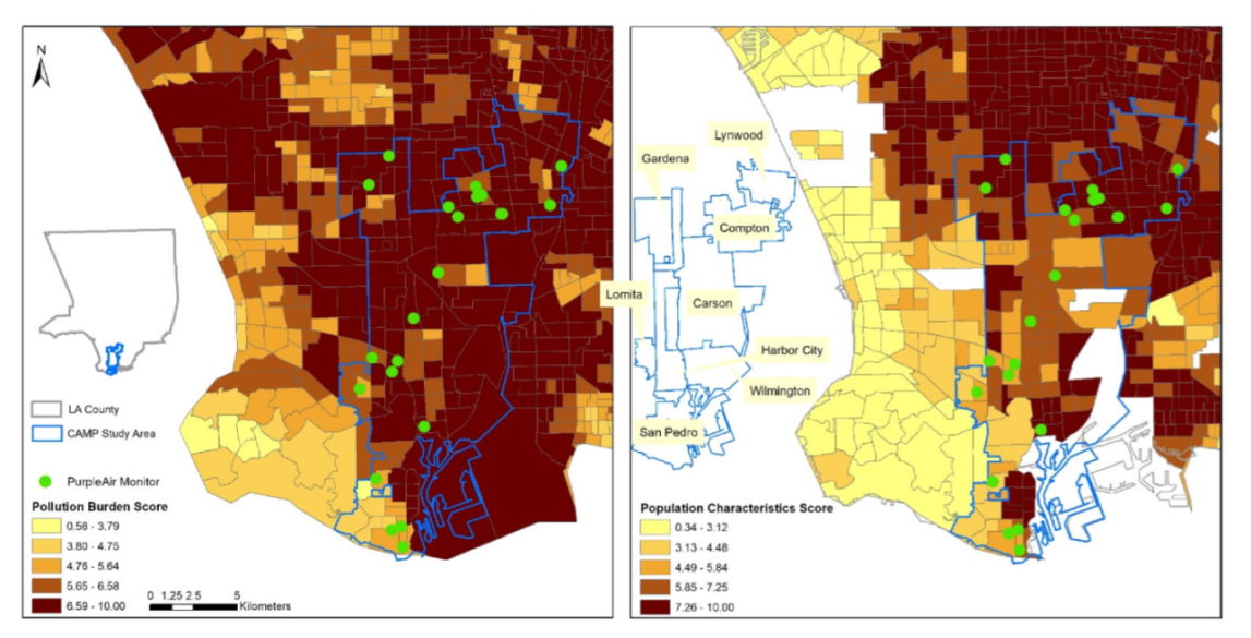
2.1. Study Area

Our CAMP study area is located in LA County, a large, populous area in Southern California (~10 million population in 2343 census tracts) with a wide spectrum of socioeconomic disparities across communities [32]. According to the US EPA, among the 229 metropolitan areas, LA is one of the most polluted regions in the US [33]. The CAMP study area includes neighborhoods from 11 communities and unincorporated areas (hereafter, communities). This area (215 km2) consists of 131 census tracts with ~630,000 population around California State University, Dominguez Hills (CSUDH; located in Carson, CA and is one of the largest Hispanic Serving Institutions in the US). Most of the CAMP study area are disadvantaged communities with low income (70%) and high proportions of minorities (56% Hispanic, 14% African American, and 13% Asian American) and susceptible populations (13% aged above 65 years old and 13% below 10 years old) with disproportionate environmental pollution burdens [32]. The area is also surrounded by several major interstate and state highways (e.g., State Route 91, Interstate 710, Interstate 110, and Interstate 105). Figure 1 shows the CAMP study area with the pollution burden and population characteristics.

2.2. Participant Recruitment

Our CAMP study team reached out to university students, faculty, alumni, and connected organizations via email to recruit resident participants from the 11 targeted communities; a total of 66 residents responded with strong interest. These residents were further selected to balance the number of selected residents in each community, neighboring transportation facilities and land uses, and distance among each household. This process resulted in 22 participants from 8 communities (i.e., Carson, Compton, Gardena, Harbor City, Lomita, Lynwood, San Pedro, and Wilmington), and about 85% were from disadvantaged communities according to the CalEnviroScreen 4.0, a tool to identify California communities that are disproportionately burdened by various sources of pollution [32]. Our study received the CSUDH Institutional Review Board approval (20-255) on 29 April 2021.

2.3. Monitoring Campaign

As one of the most popular and reliable low-cost sensor networks, PurpleAir sensors have been commonly used by universities, industrial organizations, and government air districts to effectively measure community-level air pollution using a light-scattering technique (www2.purpleair.com). One PurpleAir low-cost sensor unit was installed outside of each participant’s home (e.g., backyard, porch); each household was monitored for at least two weeks to characterize exposures for weekdays and weekends in both the summer (2 June to 27 August) and winter of 2021 (29 October to 13 December 2021). The primary goal was to track PM2.5 exposure across different time periods and households among disadvantaged communities.

2.4. Quality Assurance and Quality Control (QA/QC)

Various studies have found that PurpleAir sensors were well correlated with regulatory-grade instruments [34,35] and could be carefully calibrated to offer valuable exposure information [24,27,36]. We applied a rigorous QA/QC procedure to process the raw measurements from the CAMP study. Each PurpleAir sensor includes two sensor channels, but studies suggested that both channels generally agreed well [24,27]. Therefore, we primarily used measurements from Channel A. While these types of low-cost sensors are sensitive to relative humidity, temperature, and particle coincidence [37], a recently developed national PurpleAir correction equation found that a correction equation with an additive relative humidity term showed the best performance [27]. Therefore, our correction equation included a relative humidity term. Since the national correction equation was created based on collocated monitoring data across diverse regions in 16 states in the US, we instead applied a local hourly correction equation by using a PurpleAir sensor collocated with a regulatory-grade monitor (ID: 060371302) of South Coast Air Quality Management District (South Coast AQMD) in the City of Compton, one of the communities within our study area; the data from January to June 2021 were extracted considering data availability. The raw PurpleAir 2 min measurements were aggregated into hourly data. Then, we used the local hourly correction equation to adjust all hourly measurements of the CAMP study.

2.5. Data Analysis

We analyzed the CAMP PM2.5 measurements of the 22 households among disadvantaged communities to identify: (1) the air pollution exposure across space and time and (2) the relationship between the total PM2.5 measurements and diesel PM emissions. The overarching goal was to evaluate how residents from disadvantaged communities were exposed to ambient air pollution and how measures could be taken to relieve the pollution exposure.
To explore how PM2.5 exposure varied across communities with different built-environment and socioeconomic conditions, we calculated the community-level average PM2.5 concentrations during all monitoring days. We also compared the community-level average concentrations to the major indicators assembled from the CalEnviroScreen 4.0, namely traffic density, poverty, unemployment, housing-burdened low-income households, population characteristics, and percent of racial/ethnic population in the census tract level. Table S1 shows the detailed description of all assembled variables. To identify how PM2.5 exposure changed across different time periods, we summarized the calibrated measurements based on multiple time periods, including the hour of the day, the hour of the day by season, the hour of the day by weekday vs. weekends, and day of the week.
While evaluating the spatial and temporal patterns of air pollution exposure is significant for disadvantaged communities, exploring measures that could be implemented to reduce the exposure is also needed, especially considering that these communities are surrounded by heavy transportation facilities (e.g., freeways) and activities (e.g., warehousing). While we were aware that PM2.5 concentrations were associated with a variety of emission sources, including wildfire events, industrial facilities, and traffic activities, this study aimed to identify the traffic-related component based on the familiarity with the local environments. Firstly, we compared the CAMP PM2.5 measurements (from June to December) to the annual PM2.5 concentrations from the CalEnviroScreen 4.0 of the 22 households to check the spatial patterns of our ~one-month measurements and the annual concentrations. Secondly, we used the Pearson correlation to explore how traffic-related air pollution is associated with the ambient measurements, and we compared a traditional traffic measurement proxy (i.e., distance to nearest highway calculated from the US Census Bureau) as well as the diesel PM emissions (extracted from the CalEnviroScreen 4.0) with the CAMP PM2.5 measurements; diesel PM represents exhaust from on-road (e.g., trucks, buses) and off-road (e.g., trains, ships) sources with diesel engines. Additionally, we ranked the 22 households by the CAMP PM2.5 concentrations and the diesel PM emissions separately. We calculated delta rank (CAMP rank minus diesel rank) to assess how the diesel emissions were aligned with the ambient PM2.5 measurements. These analyses allowed for exploring air pollution exposure in our targeted disadvantaged communities beyond citizen-science-based monitoring campaigns, reflecting effective strategies to resolve exposure disparities.

3. Results and Discussion

Our local hourly correction equation for the PurpleAir measurements is y = 0.78x − 0.10rh + 7.6 (R2: 0.87); x represents raw hourly PurpleAir measurements, y represents adjusted hourly PurpleAir measurements, and rh represents relative humidity (see Figure S1). Our QA/QC procedure resulted in 18,034 h of ambient PM2.5 concentrations across the 22 households in the study area from June to December 2021. The average PM2.5 concentrations during the entire monitoring period were 18.8 µg/m3 (see Table S2). Below, we present the major findings of the spatial and temporal patterns of PM2.5 exposure as well as the relationship between traffic-related air pollution emission and the ambient PM2.5 concentrations.

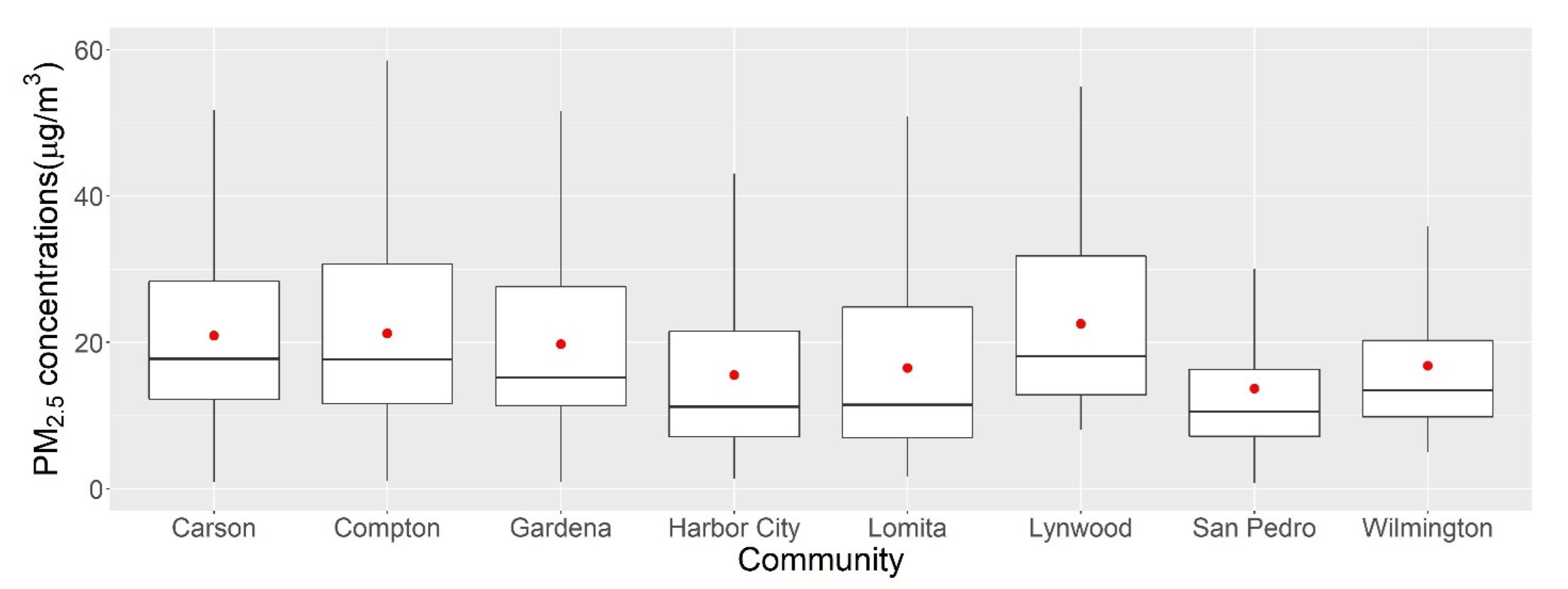
3.1. Spatial Patterns

One of our goals was to evaluate the intra-urban variations in PM2.5 exposure in the study area. Figure 2 shows the distribution and statistics of hourly PM2.5 concentrations during the two monitoring seasons by community. Lynwood (north of our study area) showed the highest average concentrations and larger variations compared with the lowest values in San Pedro (south of our study area); this result is presumably attributable to the fact that our monitored household in Lynwood was located between westbound I-710 and southbound I-105, two of the major highways in the area. This finding suggests that Lynwood may be heavily impacted by on-road mobile source emissions over time, consistent with the finding of another local study [38]. While San Pedro is located near the Port of LA, a study has found that freeway emissions were the major sources of PM2.5 and had much higher emission rates (2–5 times) compared with sources at the Port of LA [39]. This pattern was also consistent with another study reporting lower PM2.5 concentrations near the ocean [40]. However, it should be noted that the scarce number (one household in Lynwood and three households in San Pedro) and different surrounding environments (near or away from highway or ocean) of the monitored households may not fully represent community exposure.
We further explored the relationship between the community-level average exposure and the environmental and socioeconomic factors to evaluate the spatial differences. Figure 3 shows the positive correlations of household CAMP PM2.5 concentrations and percentiles of traffic density, poverty, unemployment, and housing burden (the Pearson correction coefficient (r): 0.44–0.58). This means communities with denser road networks are more likely to be exposed to higher PM2.5 concentrations, consistent with the findings of other studies [41,42,43]. Communities that are burdened by higher rates of unemployment, poverty, and housing tend to be exposed to higher PM2.5 concentrations, suggesting potential exposure disparities for disadvantaged communities, as described in other studies [44,45]. Such disparities may be attributable to the disproportionate distribution of PM-emitting facilities [46] and on-road traffic emissions [41].
Similarly, Figure 4 shows the correlations of residential outdoor PM2.5 concentrations and percentiles of population characteristics as well as the percentage of Hispanic, White, and African American population. The CAMP PM2.5 concentrations showed a strong positive association with percentiles of population characteristics (r: 0.72), and with percentages of Hispanic and African American populations (r: 0.33–0.45), again indicating that communities with a higher people of color population are exposed to poorer air quality [6,8,47,48]. In comparison, the CAMP PM2.5 concentrations were negatively associated with the percentage of White population (r: −0.83), providing more evidence regarding air pollution exposure disparities [7,46].

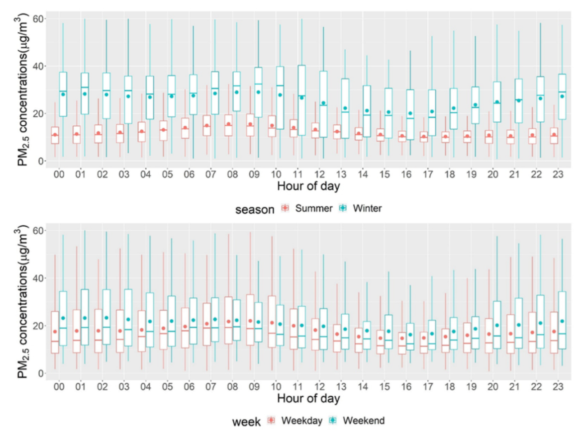
3.2. Temporal Patterns

We evaluated the temporal variations in the PM2.5 exposure of the 22 households. Figure 5 shows the distribution of hourly PM2.5 concentrations by season and weekday/weekend. In general, the average CAMP PM2.5 concentrations in winter 2021 were much higher compared with the summer concentrations (25.8 µg/m3 (winter), 12.4 µg/m3 (summer)); August had the highest concentrations during summer, and December had the highest concentrations during winter sampling. This seasonal pattern is consistent with that reported in other studies [49,50]. Particularly, one study conducted in California found that the winter PM2.5 could exceed summer PM2.5 by 68% [51]. This outcome is perhaps explained by elevated aerosol layers that were not detected by ground-level monitors. Temperature inversion during summer/winter could lead to higher PM2.5 concentrations [51]. Additionally, increasing wildfire magnitude and intensity from October to December in Southern California (with extreme seasonal winds such as Santa Ana winds) could contribute to the higher PM2.5 concentrations [23].
The average PM2.5 concentrations during weekdays were lower than those during weekends (17.9 µg/m3 (weekday) vs. 21.0 µg/m3 (weekend); see Figure S2), consistent with the results of some studies [50,52,53]. Particularly, Sunday had the highest average PM2.5 concentrations, while Tuesday had the lowest (21.8 µg/m3 (Sunday) vs. 16.5 µg/m3 (Tuesday); see Figure S3). However, other studies identified higher PM2.5 concentrations during weekdays [54,55]. A possible explanation may be that there were more travels over weekends during the COVID-19 pandemic across this area.
In terms of the hour-of-day patterns, generally, 9:00 am and 11:00 pm had peak PM2.5 concentrations and variations, while 4:00 pm had off-peak concentrations (see Figure S4). However, the between-hour PM2.5 data were much smoother than the within-hour data. This variation further reflects the spatial and temporal variations between each community (see Figure S5). For example, Lynwood had higher hourly PM2.5 concentrations compared with other communities; the peak hours were around noon. In comparison, the peak hours in Wilmington were around morning time. These outcomes are likely because residents from these disadvantaged communities may have different working shifts with greater car ownership and usage than the regional average. Additionally, disadvantaged communities are often in proximity to warehouses with high volumes of truck traffic, especially during nighttime [56,57]. Other outdoor activities during weekends or nighttime (e.g., barbecue, lawn mowing) may be important anthropogenic sources contributing to high PM2.5 concentrations. Overall, our study area may represent valuable temporal patterns among disadvantaged communities and communities in proximity to traffic segments and ports, which warrants further studies.

3.3. Temporal Patterns

We tested how our CAMP PM2.5 measurements were aligned with the annual PM2.5 concentrations, traffic-related proxy, as well as diesel emissions from CalEnviroScreen 4.0 (see Figure 6). Overall, the CAMP measurements were consistent with the annual concentrations (r: 0.89), indicating that our ~one-month measurements during two seasons were representative of the annual patterns, which agrees with one of the exposure assessment studies—the European Study of Cohorts for Air Pollution Effects (ESCAPE) [58,59]. Importantly, this finding suggests that air quality monitoring campaigns could be strategically designed to capture the annual patterns, especially for resource-constrained communities.
We found a weak correlation between the CAMP PM2.5 measurements and the diesel PM emissions (r: 0.12). This is an indication that traffic emissions are not the only sources for our study area; studies on the source apportionment of urban PM2.5 are needed to interpret the source profiles [60]. Additionally, more campaigns targeting traffic-related air pollution (e.g., black carbon; a marker for traffic particles) are needed to improve our understanding of traffic-related emissions in disadvantaged communities. Similarly, we found no correlation between the CAMP PM2.5 measurements and distance to the nearest highway (r: −0.02). However, there was a weak, negative correlation between distance to the nearest highway and the diesel PM emissions (r: −0.44). While distance to the nearest highway has commonly been used as a proxy for ambient PM2.5 [61] or traffic-related pollutants in particular [62,63], this was not obviously identified in our study, indicating that it may not well represent the traffic-related air pollution concentrations in our context. Therefore, additional proxies (e.g., traffic counts, road density) as well as more traffic-related air pollution monitoring campaigns are recommended to better characterize air pollution exposure across disadvantaged communities.
We further developed a Sankey plot to explore how the ranks of the CAMP PM2.5 concentrations and diesel PM emissions of the 22 households differed (see Figure 7). In general, most households had different ranks between ambient concentrations and diesel emissions, indicating that these households may be exposed to additional sources (e.g., passenger vehicles, industrial facilities) and are impacted by various emission reduction factors and air pollution transport processes [64]. Positive delta rank values suggest that some emission reduction and transport processes were more likely to alleviate the ambient PM2.5 exposure, while negative delta rank values suggest that additional emission sources might contribute to the ambient PM2.5 concentrations of the households.
These scenarios of delta rank values may have been reflected by the surrounding environments. For example, for a household with a delta rank value of 14 (in Wilmington), the nearest distance to the park (330 m) and sea (800 m) may explain the low ambient PM2.5 rank through emission absorbing and reduction, while the nearest distance to highway (350 m) suggests large volumes of trucks that are associated with heavy diesel PM emissions. In comparison, for a household with a delta rank value of −15 (in Compton), the nearest distance to the airport (320 m) possibly explains the additional impacts of these emission sources. Other households are surrounded by a microscale built environment, including a complex of land uses of industrial, residential, and commercial, as well as open spaces and traffic facilities and intersections, which could contribute to their nearby ambient PM2.5 concentrations [65,66].

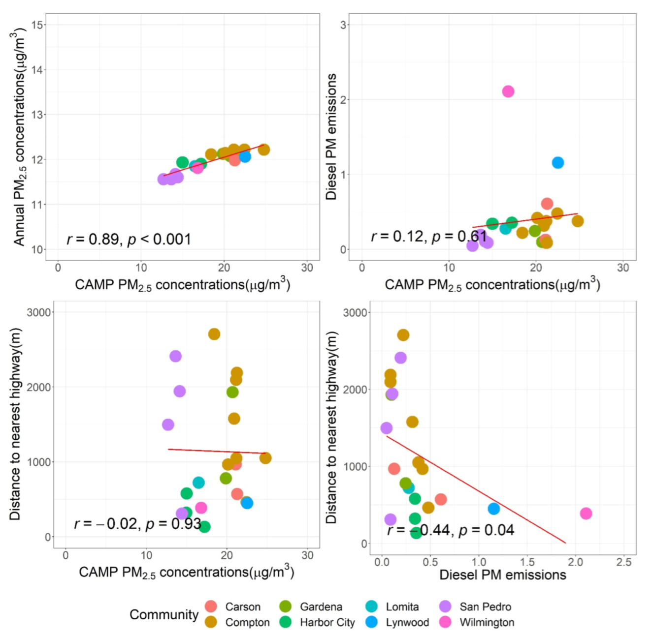
3.4. Implications for Exposure Assessment across Disadvantaged Communities

Developing reliable air monitoring campaigns is an important goal for tracking air pollution exposure. There are a limited number of studies that leverages low-cost sensors and citizen science to conduct air pollution monitoring campaigns across disadvantaged communities. Even fewer studies assess spatial and temporal patterns to inform the best exposure assessment practices for these communities. Our citizen-science-based low-cost monitoring campaign identified different PM2.5 concentrations and variations across the monitored communities, suggesting that the spatial heterogeneity of PM2.5 exposure could be better characterized within the dense networks of low-cost sensors [44,65]. We identified multiple positive/negative correlations between residential outdoor PM2.5 concentrations and socioeconomic status, as well as the surrounding built environment. With a limited number of air monitors, the choice of monitoring locations should be strategically considered to capture environments with various land uses, traffic volumes, and population characteristics with the goal of identifying exposure disparities. Our study further justifies the need to expand the low-cost sensor network across disadvantaged communities with the help of community members [10,12,47,53].
Our study showed temporal patterns that draw more attention to disadvantaged communities. We identified much higher average PM2.5 concentrations during the winter than summer of 2021, suggesting potential impacts of destructive wildfire activities and meteorological conditions in California [23,51]. The different day-of-week and hour-of-day PM2.5 concentration patterns compared with the results of previous studies indicate that these disadvantaged communities may reveal different working shifts, outdoor activities, and exposure to traffic emissions among residents. We also found that our one-month monitoring during summer and winter could be representative of the annual patterns of PM2.5. Additional monitoring is needed to evaluate the recommended number of days and seasons of monitoring for assessing long-term air pollution exposure across disadvantaged communities. Our approach of leveraging citizen science and low-cost sensors has the advantage of exploring these nuances for disadvantaged communities. For example, residents’ self-reported activities (e.g., commute pattern) and observations (e.g., wildfire smoke, traffic volumes) along with the low-cost sensor measurement would offer insights into future exposure assessment strategies.

3.5. Implications for Healthy Community Development across Disadvantaged Communities

Developing healthy communities while promoting environmental justice has gained momentum over the past few decades. A key question for urban planners is how to design cities and communities in a way that all populations would be exposed to relatively low levels of air pollution. We identified a rank difference between ambient PM2.5 concentrations and PM diesel emissions across disadvantaged communities. This finding suggests that the built environment can be targeted to reduce the exposure disparity. For example, a number of studies have found that air pollution exposure could be impacted by small-scale differences in the built environment, including traffic and road geometry [67], impervious surface [68,69], greenness [70], walkability [71], the fragmentation of urban patches [70], and other factors [19,72,73,74]. Oftentimes, disadvantaged communities are near highways, have much fewer green spaces, much greater auto dependence, poor quality pavement streets, and residential segregation patterns [14,46,48], which may be associated with adverse air pollution exposure [73] and disparities [75]. Without increased air monitoring networks among disadvantaged communities, one cannot explore such mechanisms, thus failing to eliminate built environment disparities [76], conduct air pollution exposure assessment [77], inform emission control strategies [43], and assess public health outcomes [6].

3.6. Limitations and Implications for the Development of Future Research

A limitation of our CAMP study is that only 22 participants were recruited due to a limited number of monitors, and all the measurements were collected in residential areas across the disadvantaged communities using fixed-site monitoring. An understudied topic is how the exposure assessment would be improved by the number of monitors, types of surrounding land uses and road hierarchy, and time periods of monitoring. One solution to enhance the monitoring coverage and density for disadvantaged communities is to leverage emerging satellite-based monitoring and mobile monitoring strategies [11,78,79]. Our study only measured ambient air pollution outside of each household. Future monitoring campaigns may consider monitoring both outdoor and indoor air pollution concentrations across disadvantaged communities [53], given that Southern California is very vulnerable to wildfire smoke, and older homes of disadvantaged communities tend to be leakier, with increased infiltration [80,81]. While our study shed light on the relationship between ambient air pollution concentrations and traffic-related emissions, we did not monitor pollutants that are traffic-related (e.g., black carbon) in particular. We also did not delve into source contributions to PM2.5 concentrations [82]. Future studies can explore how citizen science and low-cost sensors can be used to assess exposure to traffic-related pollutants and the source apportionment. We did not distinguish any human behaviors (e.g., types of activities, means of transportation) among different racial-ethnic groups and different wind speeds and directions across different communities. Future research could disentangle the spatial and temporal nuances of the exposure based on these factors. Another emerging challenge is how to interpret the collected measurement data and share timely information with community participants. We offered a household report to each participant in the CAMP study, but it will not be enough without a sustainable approach to democratize citizens with reliable technologies and motivation to evaluate their environmental health risks in the long run [26]. Overall, it is a concerted, ongoing effort to engage community participants, university researchers, and environmental agencies to communicate science with residents in a timely and scientific manner for improving exposure assessment and promoting environmental justice.

4. Conclusions

We leveraged citizen science and low-cost sensors to develop a community-based air monitoring program outside of 22 households across disadvantaged communities in Southern California from June 2021 to December 2021. We found that communities with a higher percentage of Hispanic and African American population and higher rates of unemployment, poverty, and housing burden were more likely to be exposed to higher PM2.5 concentrations. We also identified unique temporal (e.g., hour-of-day, day-of-week) patterns among disadvantaged communities that warrants further studies. The difference between the ambient PM2.5 concentrations and diesel PM emissions suggests that the built environment can be targeted to reduce the exposure disparity. The use of low-cost sensors with the participation of community residents offers great potential to effectively assess air pollution exposure and capture “hotspots” across space and time among disadvantaged communities. Our work could be expanded to inform emission control strategies and urban planning policies, thus improving exposure assessment, facilitating epidemiological studies, and promoting environmental justice.

Supplementary Materials

The following supporting information can be downloaded at: https://www.mdpi.com/article/10.3390/ijerph19148777/s1, Table S1: Important variables retrieved from the CalEnviroScreen 4.0; Table S2: Summary statistics of the CAMP PM2.5 concentrations during the monitoring periods; Figure S1: PurpleAir hourly correction equation using collocated monitors in the City of Compton; Figure S2: Boxplots of hourly PM2.5 concentrations by weekday vs. weekend; Figure S3: Boxplots of hour-of-day PM2.5 concentrations by day of week; Figure S4: Boxplots of hour-of-day PM2.5 concentrations; Figure S5: Boxplots of hour-of-day PM2.5 concentrations by community.

Author Contributions

Conceptualization, T.L. and Y.L. (Yisi Liu); methodology, T.L. and Y.L. (Yisi Liu); software, T.L. and G.B.-v.; validation, T.L. and A.G.; formal analysis, T.L. and Y.L. (Yisi Liu); investigation, T.L., A.G. and G.B.-v.; data curation, T.L., A.G., G.B.-v., M.W. and Y.L. (Yang Li); writing—original draft preparation, T.L. and Y.L. (Yisi Liu); writing—review and editing, T.L., Y.L. (Yisi Liu), A.G., G.B.-v., M.W., Y.L. (Yang Li), B.H., J.X. and K.C.; visualization, M.W., Y.L. (Yang Li), B.H. and J.X.; project administration, T.L.; funding acquisition, T.L. All authors have read and agreed to the published version of the manuscript.

Funding

This research was funded by the Research, Scholarship, and Creative Activity (RSCA) Awards and the Faculty Legacy Fund at California State University, Dominguez Hills.

Institutional Review Board Statement

This study was approved by the Institutional Review Board of the California State University, Dominguez Hills (approval number: 20-255; approval date: 29 April 2021).

Informed Consent Statement

Informed consent was obtained from all subjects involved in the study.

Data Availability Statement

The data presented in this study are available upon request from the corresponding author.

Acknowledgments

We would like to thank all the committed community participants of the CAMP study. We also thank Cindy Munoz who helped collected the field data.

Conflicts of Interest

The authors declare no conflict of interest.

References

  1. World Health Organization (WHO). WHO Global Ambient Air Quality Database (Update 2018); WHO: Geneva, Switzerland, 2018.
  2. Cohen, A.J.; Brauer, M.; Burnett, R.; Anderson, H.R.; Frostad, J.; Estep, K.; Balakrishnan, K.; Brunekreef, B.; Dandona, L.; Dandona, R.; et al. Estimates and 25-Year Trends of the Global Burden of Disease Attributable to Ambient Air Pollution: An Analysis of Data from the Global Burden of Diseases Study 2015. Lancet 2017, 389, 1907–1918. [Google Scholar] [CrossRef] [Green Version]
  3. Li, Z.; Liu, Y.; Lu, T.; Peng, S.; Liu, F.; Sun, J. Ecotoxicology and Environmental Safety Acute Effect of Fine Particulate Matter on Blood Pressure, Heart Rate and Related Inflammation Biomarkers: A Panel Study in Healthy Adults. Ecotoxicol. Environ. Saf. 2021, 228, 113024. [Google Scholar] [CrossRef] [PubMed]
  4. Rickenbacker, H.; Brown, F.; Bilec, M. Creating Environmental Consciousness in Underserved Communities: Implementation and Outcomes of Community-Based Environmental Justice and Air Pollution Research. Sustain. Cities Soc. 2019, 47, 101473. [Google Scholar] [CrossRef]
  5. Rosofsky, A.; Levy, J.I.; Zanobetti, A.; Janulewicz, P.; Fabian, M.P. Temporal Trends in Air Pollution Exposure Inequality in Massachusetts. Environ. Res. 2018, 161, 76–86. [Google Scholar] [CrossRef]
  6. Morello-Frosch, R.; Pastor, M.; Porras, C.; Sadd, J. Environmental Justice and Regional Inequality in Southern California: Implications for Future Research. Community Res. Environ. Health Stud. Sci. Advocacy Ethics 2017, 110, 205–218. [Google Scholar] [CrossRef] [Green Version]
  7. Liu, J.; Clark, L.P.; Bechle, M.J.; Hajat, A.; Kim, S.Y.; Robinson, A.L.; Sheppard, L.; Szpiro, A.A.; Marshall, J.D. Disparities in Air Pollution Exposure in the United States by Race/Ethnicity and Income, 1990–2010. Environ. Health Perspect. 2021, 129, 127005. [Google Scholar] [CrossRef]
  8. Tessum, C.W.; Paolella, D.A.; Chambliss, S.E.; Apte, J.S.; Hill, J.D.; Marshall, J.D. PM2.5 Polluters Disproportionately and Systemically Affect People of Color in the United States. Sci. Adv. 2021, 7, eabf4491. [Google Scholar] [CrossRef]
  9. Jorgenson, A.K.; Hill, T.D.; Clark, B.; Thombs, R.P.; Ore, P.; Balistreri, K.S.; Givens, J.E. Power, Proximity, and Physiology: Does Income Inequality and Racial Composition Amplify the Impacts of Air Pollution on Life Expectancy in the United States? Environ. Res. Lett. 2020, 15, 024013. [Google Scholar] [CrossRef]
  10. deSouza, P.; Kinney, P.L. On the Distribution of Low-Cost PM2.5 Sensors in the US: Demographic and Air Quality Associations. J. Expo. Sci. Environ. Epidemiol. 2021, 31, 514–524. [Google Scholar] [CrossRef]
  11. Sullivan, D.M.; Krupnick, A. Using Satellite Data to Fill the Gaps in the US Air Pollution Monitoring Network. Resour. Future Work. Pap. 2018, 18. Available online: https://www.rff.org/publications/working-papers/using-satellite-data-to-fill-the-gaps-in-the-us-air-pollution-monitoring-network/ (accessed on 29 August 2021).
  12. Feinberg, S.N.; Williams, R.; Hagler, G.; Low, J.; Smith, L.; Brown, R.; Garver, D.; Davis, M.; Morton, M.; Schaefer, J.; et al. Examining Spatiotemporal Variability of Urban Particulate Matter and Application of High-Time Resolution Data from a Network of Low-Cost Air Pollution Sensors. Atmos. Environ. 2019, 213, 579–584. [Google Scholar] [CrossRef]
  13. Bi, J.; Stowell, J.; Seto, E.Y.W.; English, P.B.; Al-Hamdan, M.Z.; Kinney, P.L.; Freedman, F.R.; Liu, Y. Contribution of Low-Cost Sensor Measurements to the Prediction of PM2.5 Levels: A Case Study in Imperial County, California, USA. Environ. Res. 2020, 180, 108810. [Google Scholar] [CrossRef] [PubMed]
  14. Woo, B.; Kravitz-Wirtz, N.; Sass, V.; Crowder, K.; Teixeira, S.; Takeuchi, D.T. Residential Segregation and Racial/Ethnic Disparities in Ambient Air Pollution. Race Soc. Probl. 2019, 11, 60–67. [Google Scholar] [CrossRef] [PubMed]
  15. Xu, Y.; Jiang, S.; Li, R.; Zhang, J.; Zhao, J.; Abbar, S.; González, M.C. Unraveling Environmental Justice in Ambient PM 2.5 Exposure in Beijing: A Big Data Approach. Comput. Environ. Urban Syst. 2019, 75, 12–21. [Google Scholar] [CrossRef]
  16. Hall, E.S.; Kaushik, S.M.; Vanderpool, R.W.; Duvall, R.M.; Beaver, M.R.; Long, R.W.; Solomon, P.A. Federal Reference Method (FRM), Federal Equivalent Method (FEM), National Ambient Air Quality Standards (NAAQS), Sensors; Federal Reference Method (FRM), Federal Equivalent Method (FEM), National Ambient Air Quality Standards (NAAQS), Sensors. Am. J. Environ. Eng. 2014, 4, 147–154. [Google Scholar] [CrossRef]
  17. Jiao, W.; Hagler, G.; Williams, R.; Sharpe, R.; Brown, R.; Garver, D.; Judge, R.; Caudill, M.; Rickard, J.; Davis, M.; et al. Community Air Sensor Network (CAIRSENSE) Project: Evaluation of Low-Cost Sensor Performance in a Suburban Environment in the Southeastern United States. Atmos. Meas. Tech. 2016, 9, 5281–5292. [Google Scholar] [CrossRef] [Green Version]
  18. English, P.B.; Richardson, M.J.; Garzón-Galvis, C. From Crowdsourcing to Extreme Citizen Science: Participatory Research for Environmental Health. Annu. Rev. Public Health 2018, 39, 335–350. [Google Scholar] [CrossRef] [PubMed] [Green Version]
  19. Lu, T.; Lansing, J.; Zhang, W.; Bechle, M.J.; Hankey, S. Land Use Regression Models for 60 Volatile Organic Compounds: Comparing Google Point of Interest (POI) and City Permit Data. Sci. Total Environ. 2019, 677, 131–141. [Google Scholar] [CrossRef] [PubMed]
  20. Perelló, J.; Cigarini, A.; Vicens, J.; Bonhoure, I.; Rojas-Rueda, D.; Nieuwenhuijsen, M.J.; Cirach, M.; Daher, C.; Targa, J.; Ripoll, A. Large-Scale Citizen Science Provides High-Resolution Nitrogen Dioxide Values and Health Impact While Enhancing Community Knowledge and Collective Action. Sci. Total Environ. 2021, 789, 147750. [Google Scholar] [CrossRef]
  21. Varaden, D.; Leidland, E.; Lim, S.; Barratt, B. “I Am an Air Quality Scientist”–Using Citizen Science to Characterise School Children’s Exposure to Air Pollution. Environ. Res. 2021, 201, 111536. [Google Scholar] [CrossRef] [PubMed]
  22. Bi, J.; Wildani, A.; Chang, H.H.; Liu, Y. Incorporating Low-Cost Sensor Measurements into High-Resolution PM2.5 Modeling at a Large Spatial Scale. Environ. Sci. Technol. 2020, 54, 2152–2162. [Google Scholar] [CrossRef] [PubMed]
  23. Lu, Y.; Giuliano, G.; Habre, R. Estimating Hourly PM2.5 Concentrations at the Neighborhood Scale Using a Low-Cost Air Sensor Network: A Los Angeles Case Study. Environ. Res. 2021, 195, 110653. [Google Scholar] [CrossRef] [PubMed]
  24. Lu, T.; Bechle, M.J.; Wan, Y.; Presto, A.A.; Hankey, S. Using Crowd-Sourced Low-Cost Sensors in a Land Use Regression of PM2.5 in 6 US Cities. Air Qual. Atmos. Health 2022, 15, 667–678. [Google Scholar] [CrossRef]
  25. Mahajan, S.; Kumar, P.; Pinto, J.A.; Riccetti, A.; Schaaf, K.; Camprodon, G.; Smári, V.; Passani, A.; Forino, G. A Citizen Science Approach for Enhancing Public Understanding of Air Pollution. Sustain. Cities Soc. 2020, 52, 101800. [Google Scholar] [CrossRef]
  26. Austen, K. Pollution Patrol. Nature 2015, 517, 136–138. [Google Scholar] [CrossRef] [Green Version]
  27. Barkjohn, K.K.; Gantt, B.; Clements, A.L. Development and Application of a United States-Wide Correction for PM 2.5 Data Collected with the PurpleAir Sensor. Atmos. Meas. Tech. 2021, 14, 4617–4637. [Google Scholar] [CrossRef]
  28. Hasheminassab, S.; Daher, N.; Saffari, A.; Wang, D.; Ostro, B.D.; Sioutas, C. Spatial and Temporal Variability of Sources of Ambient Fine Particulate Matter (PM2.5) in California. Atmos. Chem. Phys. 2014, 5, 12085–12097. [Google Scholar] [CrossRef] [Green Version]
  29. Lurmann, F.; Avol, E.; Gilliland, F.; Lurmann, F.; Avol, E.; Gilliland, F. Emissions Reduction Policies and Recent Trends in Southern California’s Ambient Air Quality Emissions Reduction Policies and Recent Trends in Southern California ’ s Ambient Air Quality. J. Air Waste Manag. Assoc. 2015, 65, 324–335. [Google Scholar] [CrossRef] [Green Version]
  30. Johnston, J.E.; Juarez, Z.; Navarro, S.; Hernandez, A.; Gutschow, W. Youth Engaged Participatory Air Monitoring: A ‘Day in the Life’ in Urban Environmental Justice Communities. Int. J. Environ. Res. Public Health 2020, 17, 93. [Google Scholar] [CrossRef] [Green Version]
  31. Mullen, C.; Flores, A.; Grineski, S.; Collins, T. Exploring the Distributional Environmental Justice Implications of an Air Quality Monitoring Network in Los Angeles County. Environ. Res. 2022, 206, 112612. [Google Scholar] [CrossRef]
  32. The Office of Environmental Health Hazard Assessment (OEHHA) CalEnviroScreen 4.0. Available online: https://oehha.ca.gov/calenviroscreen/report/calenviroscreen-40 (accessed on 28 August 2021).
  33. US Environmental Protection Agency (US EPA) California Nonattainment/Maintenance Status for Each County by Year for All Criteria Pollutants. Available online: https://www3.epa.gov/airquality/greenbook/anayo_ca.html (accessed on 29 August 2021).
  34. Brauer, M.; Lee, M. Evaluation of Portable Air Quality Sensors at the Vancouver (Clark Drive) near-Road Air Quality Monitoring Site. 2018. Available online: https://open.library.ubc.ca/soa/cIRcle/collections/facultyresearchandpublications/52383/items/1.0380965 (accessed on 29 March 2021).
  35. South Coast Air Quality Management District Field Evaluation Purple Air PM Sensor Background. Available online: http://www.aqmd.gov/docs/default-source/aq-spec/field-evaluations/purple-air-pa-ii---field-evaluation.pdf?sfvrsn=2 (accessed on 23 May 2020).
  36. Malings, C.; Tanzer, R.; Hauryliuk, A.; Saha, P.K.; Allen, L.; Presto, A.A.; Subramanian, R.; Malings, C.; Tanzer, R.; Hauryliuk, A.; et al. Fine Particle Mass Monitoring with Low-Cost Sensors: Corrections and Long-Term Performance Evaluation Term Performance Evaluation. Aerosol Sci. Technol. 2020, 54, 160–174. [Google Scholar] [CrossRef]
  37. Xu, R. Particuology Light Scattering: A Review of Particle Characterization Applications. Particuology 2015, 18, 11–21. [Google Scholar] [CrossRef]
  38. Bishop, G.A. Three Decades of On-Road Mobile Source Emissions Reductions in South Los Angeles. J. Air Waste Manag. Assoc. 2019, 69, 967–976. [Google Scholar] [CrossRef]
  39. Mousavi, A.; Sowlat, M.H.; Hasheminassab, S.; Pikelnaya, O.; Polidori, A.; Ban-weiss, G.; Sioutas, C. Impact of Particulate Matter (PM) Emissions from Ships, Locomotives, and Freeways in the Communities near the Ports of Los Angeles (POLA) and Long Beach (POLB) on the Air Quality in the Los Angeles County. Atmos. Environ. 2018, 195, 159–169. [Google Scholar] [CrossRef]
  40. Hu, S.; Polidori, A.; Arhami, M.; Shafer, M.M.; Schauer, J.J.; Cho, A.; Sioutas, C. And Physics Redox Activity and Chemical Speciation of Size Fractioned PM in the Communities of the Los Angeles-Long Beach Harbor. Atmos. Che 2008, 8, 6439–6451. [Google Scholar] [CrossRef] [Green Version]
  41. Lee, H.J.; Park, H. Prioritizing the Control of Emission Sources to Mitigate PM2.5 Disparity in California. Atmos. Environ. 2020, 224, 117316. [Google Scholar] [CrossRef]
  42. Di, Q.; Kloog, I.; Koutrakis, P.; Lyapustin, A.; Wang, Y.; Schwartz, J. Assessing PM 2.5 Exposures with High Spatiotemporal Resolution across the Continental United States. Environ. Sci. Technol. 2016, 50, 4712–4721. [Google Scholar] [CrossRef] [Green Version]
  43. Lee, C. Impacts of Multi-Scale Urban Form on PM2.5 Concentrations Using Continuous Surface Estimates with High-Resolution in U. S. Metropolitan Areas. Landsc. Urban Plan. 2020, 204, 103935. [Google Scholar] [CrossRef]
  44. Cooper, N.; Green, D.; Knibbs, L.D. Inequalities in Exposure to the Air Pollutants PM2.5 and NO2 in Australia. Environ. Res. Lett. 2019, 14, 115005. [Google Scholar] [CrossRef]
  45. Hajat, A.; Hsia, C.; O’Neill, M.S. Socioeconomic Disparities and Air Pollution Exposure: A Global Review. Curr. Environ. Health Rep. 2015, 2, 440–450. [Google Scholar] [CrossRef] [Green Version]
  46. Mikati, I.; Benson, A.F.; Luben, T.J.; Sacks, J.D.; Richmond-Bryant, J. Disparities in Distribution of Particulate Matter Emission Sources by Race and Poverty Status. Am. J. Public Health 2018, 108, 480–485. [Google Scholar] [CrossRef] [PubMed]
  47. Racz, L.A.; Rish, W. Exposure Monitoring toward Environmental Justice. Integr. Environ. Assess. Manag. 2021, 18, 858–862. [Google Scholar] [CrossRef] [PubMed]
  48. Masri, S.; Cox, K.; Flores, L.; Rea, J.; Wu, J. Community-Engaged Use of Low-Cost Sensors to Assess the Spatial Distribution of PM2.5 Concentrations across Disadvantaged Communities: Results from a Pilot Study in Santa Ana, CA. Atmosphere 2022, 13, 304. [Google Scholar] [CrossRef]
  49. Chan, E.A.W.; Gantt, B.; McDow, S. The Reduction of Summer Sulfate and Switch from Summertime to Wintertime PM2.5 Concentration Maxima in the United States. Atmos. Environ. 2018, 175, 25–32. [Google Scholar] [CrossRef]
  50. Zhao, N.; Liu, Y.; Vanos, J.K.; Cao, G. Day-of-Week and Seasonal Patterns of PM2.5 Concentrations over the United States: Time-Series Analyses Using the Prophet Procedure. Atmos. Environ. 2018, 192, 116–127. [Google Scholar] [CrossRef]
  51. Lewis, J.; De Young, R.; Ferrare, R.; Allen Chu, D. Comparison of Summer and Winter California Central Valley Aerosol Distributions from Lidar and MODIS Measurements. Atmos. Environ. 2010, 44, 4510–4520. [Google Scholar] [CrossRef] [Green Version]
  52. Chen, T.; He, J.; Lu, X.; She, J.; Guan, Z. Spatial and Temporal Variations of PM2.5 and Its Relation to Meteorological Factors in the Urban Area of Nanjing, China. Int. J. Environ. Res. Public Health 2016, 13, 921. [Google Scholar] [CrossRef]
  53. Connolly, R.E.; Yu, Q.; Wang, Z.; Chen, Y.; Liu, J.Z.; Collier-oxandale, A.; Papapostolou, V.; Polidori, A.; Zhu, Y. Long-Term Evaluation of a Low-Cost Air Sensor Network for Monitoring Indoor and Outdoor Air Quality at the Community Scale. Sci. Total Environ. 2022, 807, 150797. [Google Scholar] [CrossRef]
  54. Motallebi, N.; Tran, H.; Croes, B.E.; Larsen, L.C. Day-of-Week Patterns of Particulate Matter and Its Chemical Components at Selected Sites in California? J. Air Waste Manag. Assoc. 2003, 53, 876–888. [Google Scholar] [CrossRef] [Green Version]
  55. Lough, G.C.; Schauer, J.J.; Lawson, D.R. Day-of-Week Trends in Carbonaceous Aerosol Composition in the Urban Atmosphere. Atmos. Environ. 2006, 40, 4137–4149. [Google Scholar] [CrossRef]
  56. Yuan, Q. Environmental Justice in Warehousing Location: State of the Art. J. Plan. Lit. 2018, 33, 287–298. [Google Scholar] [CrossRef]
  57. Giuliano, G.; Brien, T.O. Reducing Port-Related Truck Emissions: The Terminal Gate Appointment System at the Ports of Los Angeles and Long Beach. Transp. Res. Part D Transp. 2007, 12, 460–473. [Google Scholar] [CrossRef]
  58. Wang, M.; Beelen, R.; Basagana, X.; Becker, T.; Cesaroni, G.; De Hoogh, K.; Dedele, A.; Declercq, C.; Dimakopoulou, K.; Eeftens, M.; et al. Evaluation of Land Use Regression Models for NO2 and Particulate Matter in 20 European Study Areas: The ESCAPE Project. Environ. Sci. Technol. 2013, 47, 4357–4364. [Google Scholar] [CrossRef] [PubMed]
  59. Eeftens, M.; Tsai, M.Y.; Ampe, C.; Anwander, B.; Beelen, R.; Bellander, T.; Cesaroni, G.; Cirach, M.; Cyrys, J.; de Hoogh, K.; et al. Spatial Variation of PM2.5, PM10, PM2.5 Absorbance and PMcoarse Concentrations between and within 20 European Study Areas and the Relationship with NO2—Results of the ESCAPE Project. Atmos. Environ. 2012, 62, 303–317. [Google Scholar] [CrossRef] [Green Version]
  60. Vallius, M.; Janssen, N.A.H.; Heinrich, J.; Hoek, G.; Ruuskanen, J.; Cyrys, J.; Van Grieken, R.; De Hartog, J.J.; Kreyling, W.G.; Pekkanen, J. Sources and Elemental Composition of Ambient PM2.5 in Three European Cities. Sci. Total Environ. 2005, 337, 147–162. [Google Scholar] [CrossRef]
  61. Auchincloss, A.H.; Diez Roux, A.V.; Dvonch, J.T.; Brown, P.L.; Barr, R.G.; Daviglus, M.L.; Goff, D.C.; Kaufman, J.D.; O’Neill, M.S. Associations between Recent Exposure to Ambient Fine Particulate Matter and Blood Pressure in the Multi-Ethnic Study of Atherosclerosis (MESA). Environ. Health Perspect. 2008, 116, 486–491. [Google Scholar] [CrossRef]
  62. Zhu, Y.; Hinds, W.C.; Kim, S.; Shen, S. Study of Ultrafine Particles near a Major Highway with Heavy-Duty Diesel Traffic. Atmos. Environ. 2002, 36, 4323–4335. [Google Scholar] [CrossRef]
  63. Karner, A.A.; Eisinger, D.S.; Niemeier, D.E.B.A. Near-Roadway Air Quality: Synthesizing the Findings from Real-World Data. Environ. Sci. Technol. 2010, 44, 5334–5344. [Google Scholar] [CrossRef]
  64. Pant, P.; Harrison, R.M. Estimation of the Contribution of Road Traf Fi c Emissions to Particulate Matter Concentrations from Fi Eld Measurements: A Review. Atmos. Environ. 2013, 77, 78–97. [Google Scholar] [CrossRef]
  65. Zhou, S.; Lin, R. Spatial-Temporal Heterogeneity of Air Pollution: The Relationship between Built Environment and on-Road PM2.5 at Micro Scale. Transp. Res. Part D 2019, 76, 305–322. [Google Scholar] [CrossRef]
  66. Hankey, S.; Marshall, J.D. Land Use Regression Models of On-Road Particulate Air Pollution (Particle Number, Black Carbon, PM2.5, Particle Size) Using Mobile Monitoring. Environ. Sci. Technol. 2015, 49, 9194–9202. [Google Scholar] [CrossRef]
  67. Farrell, W.; Weichenthal, S.; Goldberg, M.; Valois, M.; Shekarrizfard, M.; Hatzopoulou, M. Near Roadway Air Pollution across a Spatially Extensive Road and Cycling Network. Environ. Pollut. 2016, 212, 498–507. [Google Scholar] [CrossRef] [PubMed]
  68. Kashem, S.B.; Irawan, A.; Wilson, B. Evaluating the Dynamic Impacts of Urban Form on Transportation and Environmental Outcomes in US Cities. Int. J. Environ. Sci. Technol. 2014, 11, 2233–2244. [Google Scholar] [CrossRef] [Green Version]
  69. Larkin, A.; Van Donkelaar, A.; Geddes, A.; Martin, R.V.; Hystad, P. Quality in East Asia from 2000 to 2010. Environ. Sci. Technol. 2016, 50, 9142–9149. [Google Scholar] [CrossRef] [PubMed] [Green Version]
  70. Mccarty, J.; Kaza, N. Urban Form and Air Quality in the United States. Landsc. Urban Plan. 2015, 139, 168–179. [Google Scholar] [CrossRef]
  71. James, P.; Hart, J.E.; Laden, F. Neighborhood Walkability and Particulate Air Pollution in a Nationwide Cohort of Women. Environ. Res. 2015, 142, 703–711. [Google Scholar] [CrossRef] [Green Version]
  72. Chakraborty, J.; Zandbergen, P.A. Children at Risk: Measuring Racial/Ethnic Disparities in Potential Exposure to Air Pollution at School and Home. J. Epidemiol. Community Health 2007, 61, 1074–1079. [Google Scholar] [CrossRef] [Green Version]
  73. Hankey, S.; Marshall, J.D. Urban Form, Air Pollution, and Health. Curr. Environ. Health Rep. 2017, 4, 491–503. [Google Scholar] [CrossRef]
  74. Lu, T.; Marshall, J.D.; Zhang, W.; Hystad, P.; Kim, S.; Bechle, M.J.; Demuzere, M.; Hankey, S. National Empirical Models of Air Pollution Using Microscale Measures of the Urban Environment. Environ. Sci. Technol. 2021, 55, 15519–15530. [Google Scholar] [CrossRef]
  75. Gardner-Frolick, R.; Boyd, D.; Giang, A. Selecting Data Analytic and Modeling Methods to Support Air Pollution and Environmental Justice Investigations: A Critical Review and Guidance Framework. Environ. Sci. Technol. 2022, 56, 2843–2860. [Google Scholar] [CrossRef]
  76. Hutch, D.J.; Bouye, K.E.; Skillen, E.; Lee, C.; Whitehead, L.; Rashid, J.R. Collaborative Strategies to Improve Public Health Potential Strategies to Eliminate Built Environment Disparities for Disadvantaged and Vulnerable Communities. Gov. Politics Law 2011, 101, 587–595. [Google Scholar] [CrossRef]
  77. Hankey, S.; Lindsey, G.; Marshall, J.D. Population-Level Exposure to Particulate Air Pollution during Active Travel: Planning for Low-Exposure, Health-Promoting Cities. Environ. Health Perspect. 2017, 125, 527–534. [Google Scholar] [CrossRef]
  78. Hankey, S.; Sforza, P.; Pierson, M. Using Mobile Monitoring to Develop Hourly Empirical Models of Particulate Air Pollution in a Rural Appalachian Community. Environ. Sci. Technol. 2019, 53, 4305–4315. [Google Scholar] [CrossRef]
  79. Messier, K.P.; Chambliss, S.E.; Gani, S.; Alvarez, R.; Brauer, M.; Choi, J.J.; Hamburg, S.P.; Kerckho, J.; Lafranchi, B.; Lunden, M.M.; et al. Mapping Air Pollution with Google Street View Cars: E Ffi Cient Approaches with Mobile Monitoring and Land Use Regression. Environ. Sci. Technol. 2018, 52, 12563–12572. [Google Scholar] [CrossRef] [PubMed] [Green Version]
  80. Liang, Y.; Sengupta, D.; Campmier, M.J.; Lunderberg, D.M.; Apte, J.S. Wildfire Smoke Impacts on Indoor Air Quality Assessed Using Crowdsourced Data in California. Proc. Natl. Acad. Sci. USA 2021, 118, e2106478118. [Google Scholar] [CrossRef]
  81. Adamkiewicz, G.; Zota, A.R.; Fabian, M.P.; Chahine, T.; Julien, R.; Spengler, J.D. Moving Environmental Justice Indoors: Understanding Structural Influences on Residential Exposure Patterns in Low-Income Communities. Am. J. Public Health 2011, 101, 238–245. [Google Scholar] [CrossRef]
  82. Habre, R.; Girguis, M.; Urman, R.; Fruin, S.; Lurmann, F.; Shafer, M.; Gorski, P.; Franklin, M.; Mcconnell, R.; Avol, E.; et al. Contribution of Tailpipe and Non-Tailpipe Traffic Sources to Quasi-Ultrafine, Fine and Coarse Particulate Matter in Southern California. J. Air Waste Manag. Assoc. 2021, 71, 209–230. [Google Scholar] [CrossRef]
Figure 1. CAMP study area with the pollution burden and population characteristics.
Ijerph 19 08777 g001
Figure 2. Boxplots of hourly PM2.5 concentrations during summer and fall 2021 by community. The red dots indicate average concentrations. The boxes show the interquartile range (IQR). The upper whisker extends from the hinge to the largest value at most 1.5*IQR, while the lower whisker extends from the hinge to the smallest value at most 1.5*IQR.
Ijerph 19 08777 g002
Figure 3. The correlations of residential outdoor PM2.5 concentrations and percentiles of traffic density, poverty, unemployment, and housing burden.
Ijerph 19 08777 g003
Figure 4. The correlations of residential outdoor PM2.5 concentrations and percentiles of population characteristics as well as the percentage of Hispanic, White, and African American population. Population characteristics represent characteristics (e.g., health status, community features) that result in vulnerability to pollution as defined by CalEnviroScreen 4.0.
Ijerph 19 08777 g004
Figure 5. Boxplots of hour-of-day PM2.5 concentrations by season and weekday/weekend. The red/blue dots indicate average concentrations. The boxes show the interquartile range (IQR). The upper whisker extends from the hinge to the largest value at most 1.5*IQR, while the lower whisker extends from the hinge to the smallest value at most 1.5*IQR.
Ijerph 19 08777 g005
Figure 6. The comparisons of CAMP PM2.5 concentrations, annual PM2.5 concentrations, distance to nearest highway, and diesel PM emissions by community.
Ijerph 19 08777 g006
Figure 7. The rank difference between the CAMP PM2.5 rank and the diesel PM rank of the 22 households. Each line represents one household. Households ranking at the top were exposed to higher ambient PM2.5 or diesel PM emissions; households ranking at the bottom were exposed to lower ambient PM2.5 or diesel PM emissions.
Ijerph 19 08777 g007
Publisher’s Note: MDPI stays neutral with regard to jurisdictional claims in published maps and institutional affiliations.

