
The Relationship between the Outdoor School Violence Distribution and the Outdoor Campus Environment: An Empirical Study from China


Abstract
:1. Introduction
- (1)
- What are the spatial distribution characteristics of different outdoor school violence types?
- (2)
- Is there a relationship between the distribution of each outdoor school violence type and the spatial attributes (spatial configuration and spatial visibility) of the OCE? What is the relationship?
- (3)
- How do the various spatial attributes of the OCE affect the distribution of each outdoor school violence type? What are the predictors?
2. Methodology
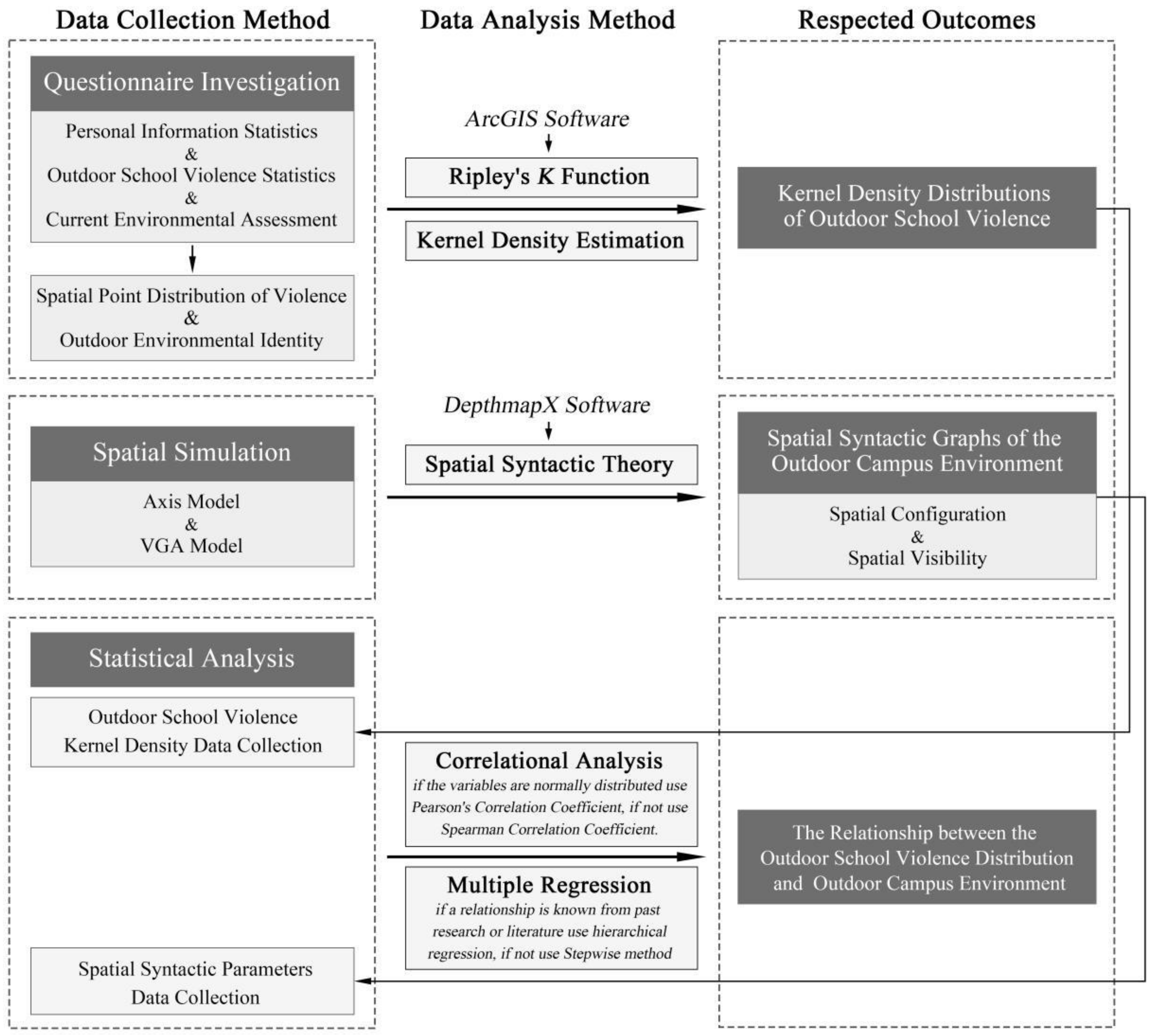
2.1. Study Design
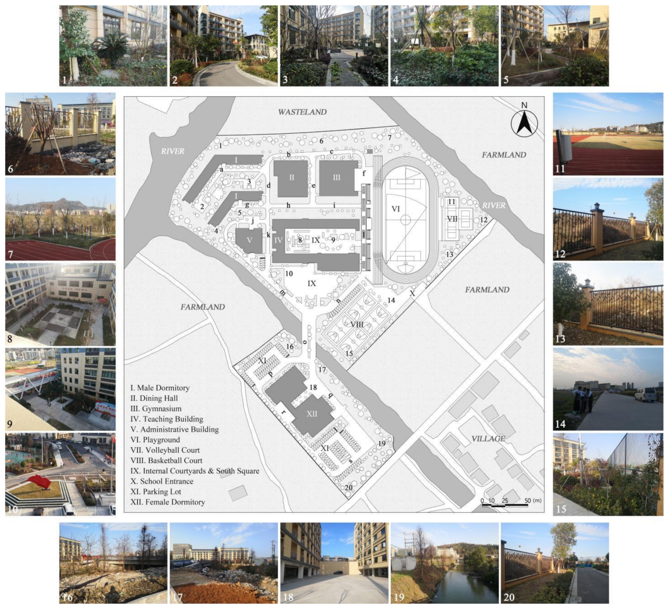
2.2. Field Site
- Universal school type: Statistics from Ministry of Education of the People’s Republic of China show that the number of boarding students in compulsory education has reached 32.765 million after 2012, accounting for 21.85% of the total number of students in school [72]. It is evident that boarding schools are common in China, and research on their school violence is somewhat applicable.
- Diversified building functions: In contrast to regular schools, boarding schools have facilities such as teaching buildings, office buildings, and gymnasiums, as well as dormitories and other facilities that serve the daily lives of students, which may increase the possibility of outdoor school violence to some extent.
- Special student population: Most of the students in boarding schools are left-behind children [73] whose parents are often in the laboring group. These students’ personalities tend to become stubborn, distrustful, lonely, and rude due to the lack of family care, as well as psychological problems such as anxiety, loneliness, and boredom that are caused by adaptation to the environment. Students in boarding schools are, therefore, a special group, with not only the general psychological characteristics of contemporary students, but also the special psychological problems of left-behind children.
- Representative violence rate: A random sample of students in different grades obtained an outdoor violence rate that reached 58.01%, which is higher than the above-mentioned violence rate in China (32.4%) and the global violence rate (32%), indicating that Case L is strikingly representative [68].
2.3. Questionnaire Investigation
2.3.1. Investigation Method
- Deletion: When faced with invalid responses throughout the questionnaire, the sample should be simply deleted.
- Partial deletion: When an individual question in a valid questionnaire had a missing response, the data for it were removed but the other valid variables were retained.
- Modify: When faced with a missing variable in a sample, it can be filled in with the mean of the remaining variables. For classification, when the missing amount was less than 5%, the overall mean of the variable was used to replace. Otherwise, the hot deck method can be used to group the valid data for that variable and choose the mean of a certain group as the value of the missing sample.
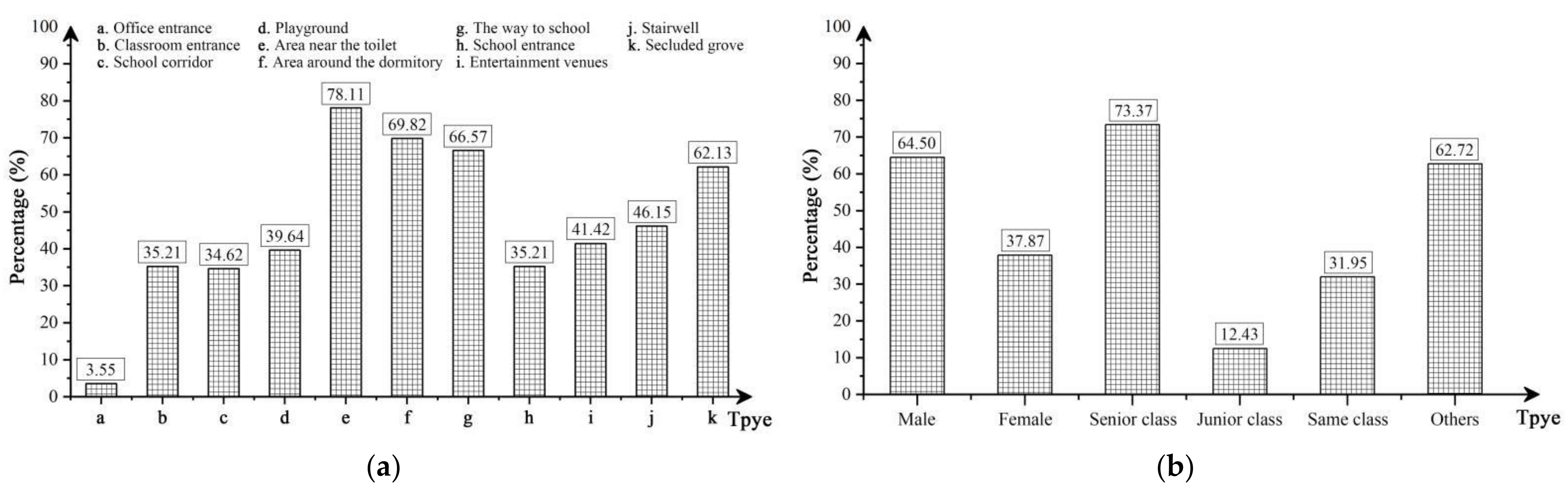
2.3.2. Investigation Findings
2.3.3. Data Handling Tools
2.4. Spatial Simulation
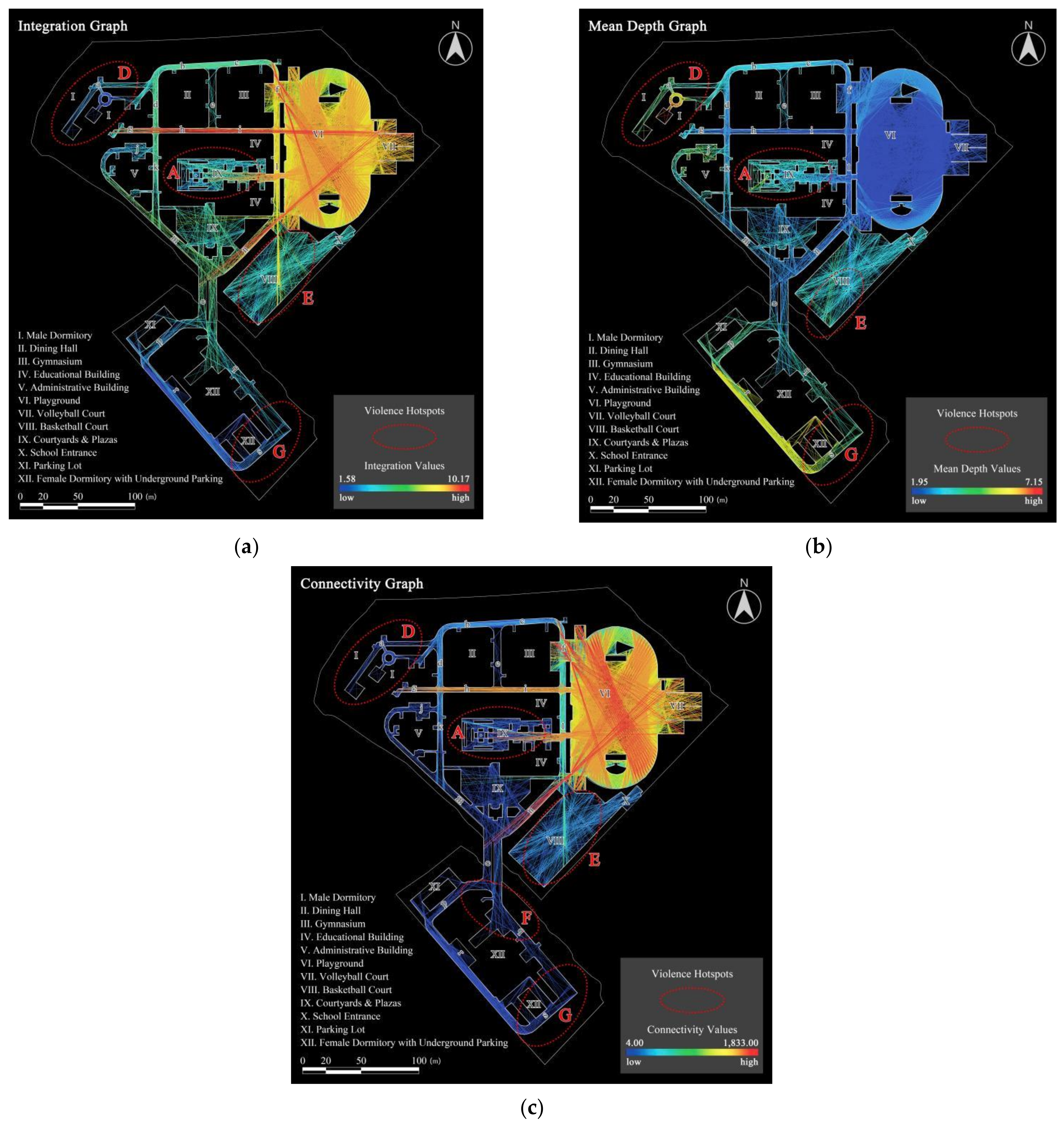
- Integration (In) represents the relationship between a space and local or overall space, that is, the accessibility of the space. The higher the In value, the higher the accessibility [73].
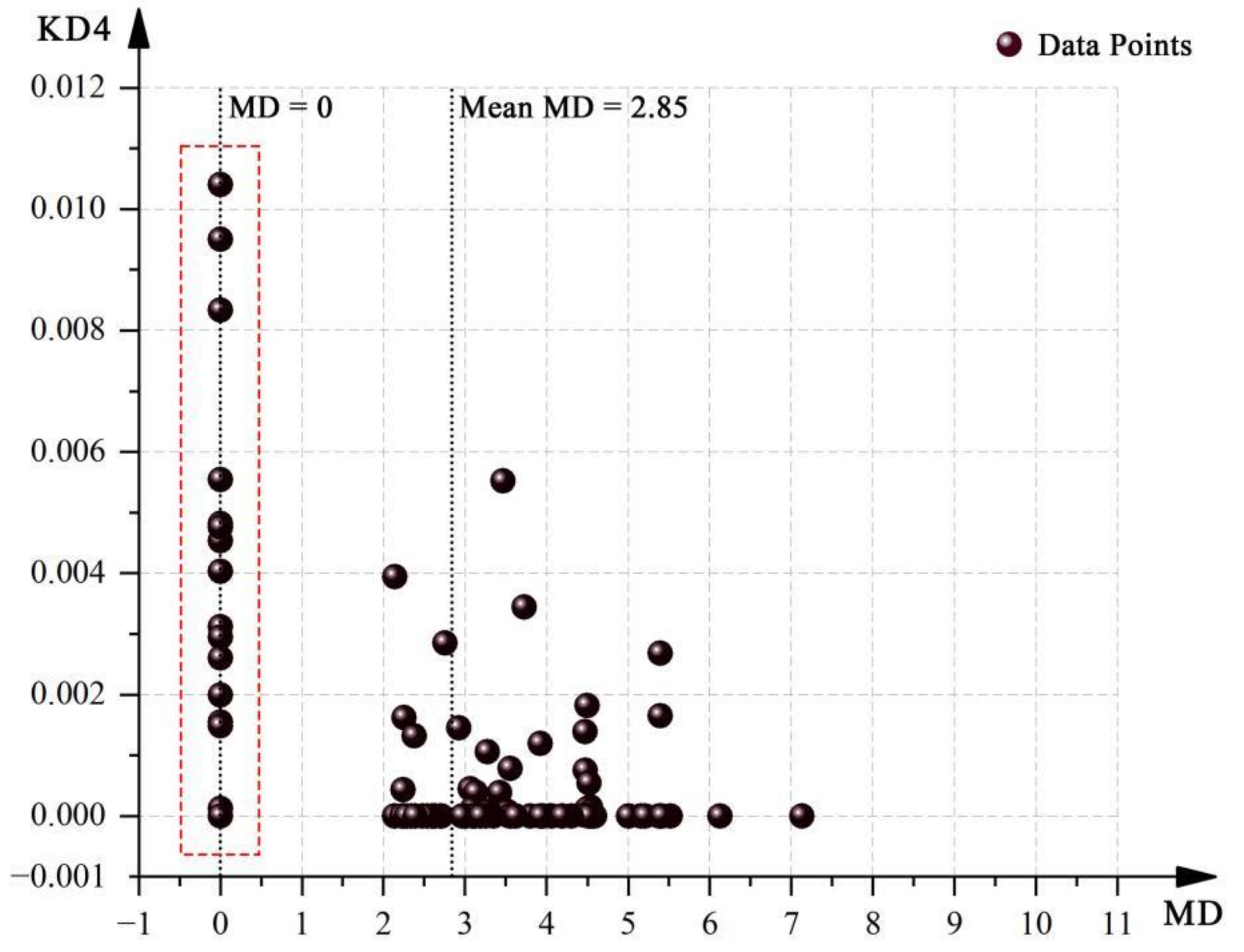
- Mean Depth (MD) indicates the number of transformations from local space to other parts of space, representing the convenience of the node in the spatial system. Higher values of MD indicate higher spatial separation [84].
- Connectivity (Con) refers to the sum of the number of spaces directly connected with the surrounding space. The higher the Con value of a space, the more spaces connected with it, characterizing as a transportation hub in the spatial system.
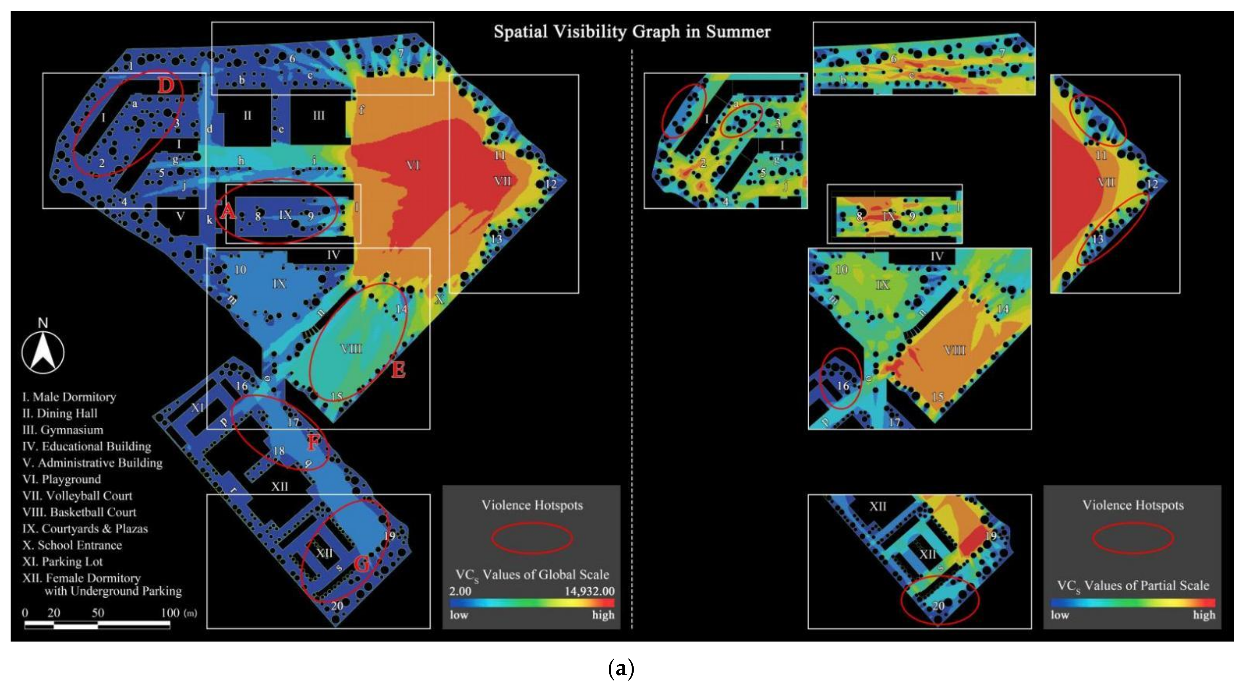
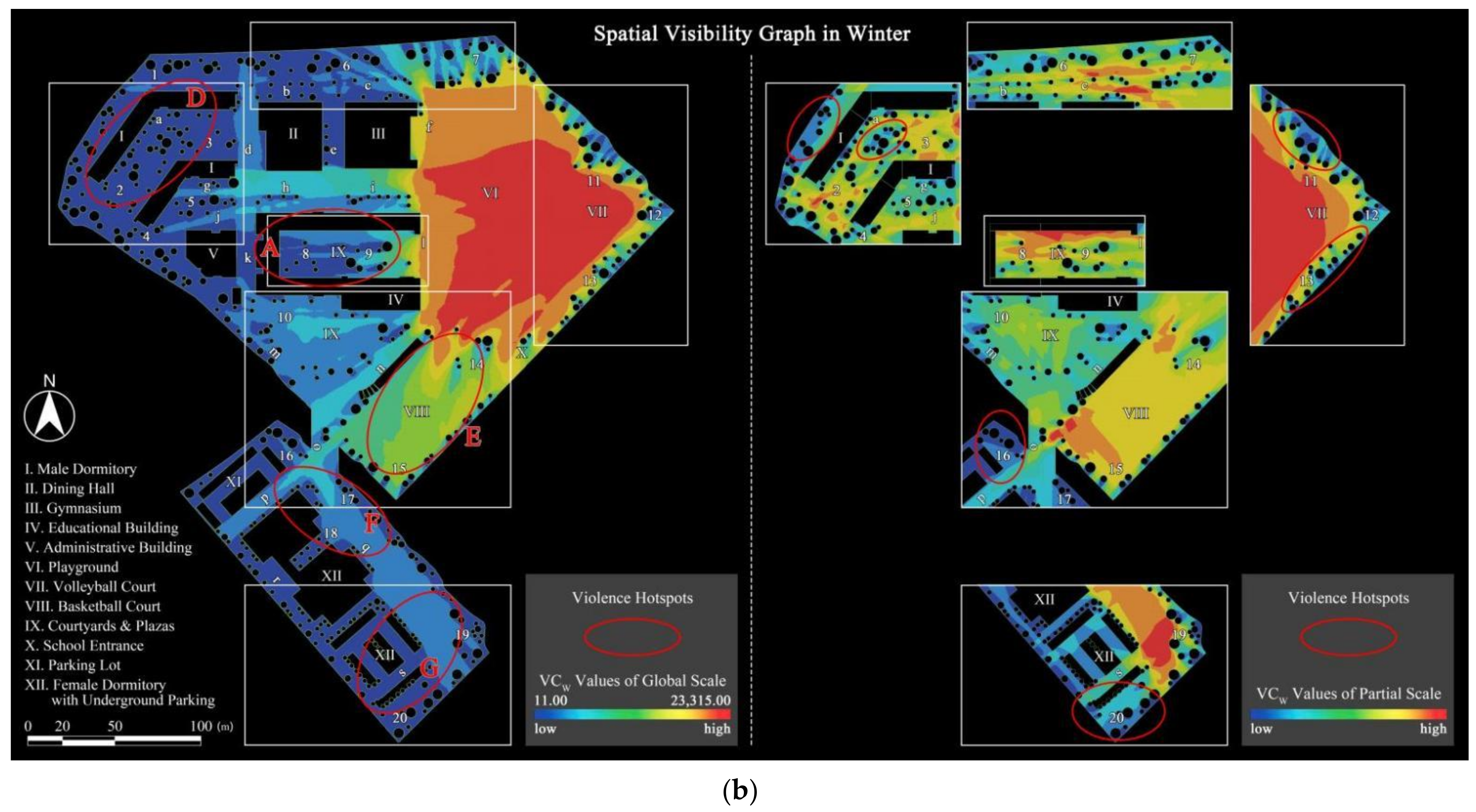
- Visibility Connectivity (VC) shows the number of other points that a point can see within its line of sight, reflecting the quality of natural surveillance provided by the outdoor environment to users or passers-by. The higher the VC value, the better the quality of surveillance or under surveillance [68].
2.5. Statistical Analysis
- Normal distribution test: It was required for all data to select the appropriate correlation coefficient through this test. After embedded in SPSS Statistics 26, the one-sample Kolmogorov–Smirnov (K-S) test thus must be performed. If the variables were normally distributed (p > 0.05), Pearson’s correlation coefficient would be used, otherwise (p ≤ 0.05), Spearman correlation coefficient should be used [86].
- Correlation analysis: With the data imported into Stata 15.1 software, the bivariate correlation analysis was carried out using the appropriate correlation coefficients for kernel density variables and spatial attribute variables, discriminated by significance p and correlation coefficient r [85]. p was used to test whether there was a statistically significant relationship between the two variables (p-values less than 0.1, 0.05, or 0.01 all indicate a correlation, denoted by *, ** and ***, respectively, in ascending order of significance). If significant, the positive and negative direction of the correlation coefficient r and the degree of correlation should be analyzed. A larger absolute value of r indicated a higher degree of correlation.
- Multiple regression analysis and model building: It was used to explore the regression relationships between outdoor school violence kernel density variables and spatial attribute variables to predict the magnitude of the effect of different spatial attribute variables on the same violence kernel density. Specifically, the hierarchical regression method was used if the relationship between certain variables can be obtained from previous literature, otherwise the stepwise method should be chosen [85]. Once the regression analysis was determined, the data were tested for covariance to prevent interactions within the variables, including two indicators of variance inflation factor (VIF) (less than 10) and tolerance (greater than 0.2). Further, the regression coefficient beta, t-test value, and significance p were selected as indicators to discriminate the regression relationship. Among them, the t-test and p-value were judged by the same criteria as the above conditions. If the absolute value of beta was greater than zero, then the independent variable can effectively predict the variation of the dependent variable, i.e., there was a significant influence relationship. Also in the hierarchical regression analysis, R2 change (the difference in R2 between two consecutive models) represented the contribution that was made by increasing the independent variable; the larger the value, the more prominent the influence relationship.
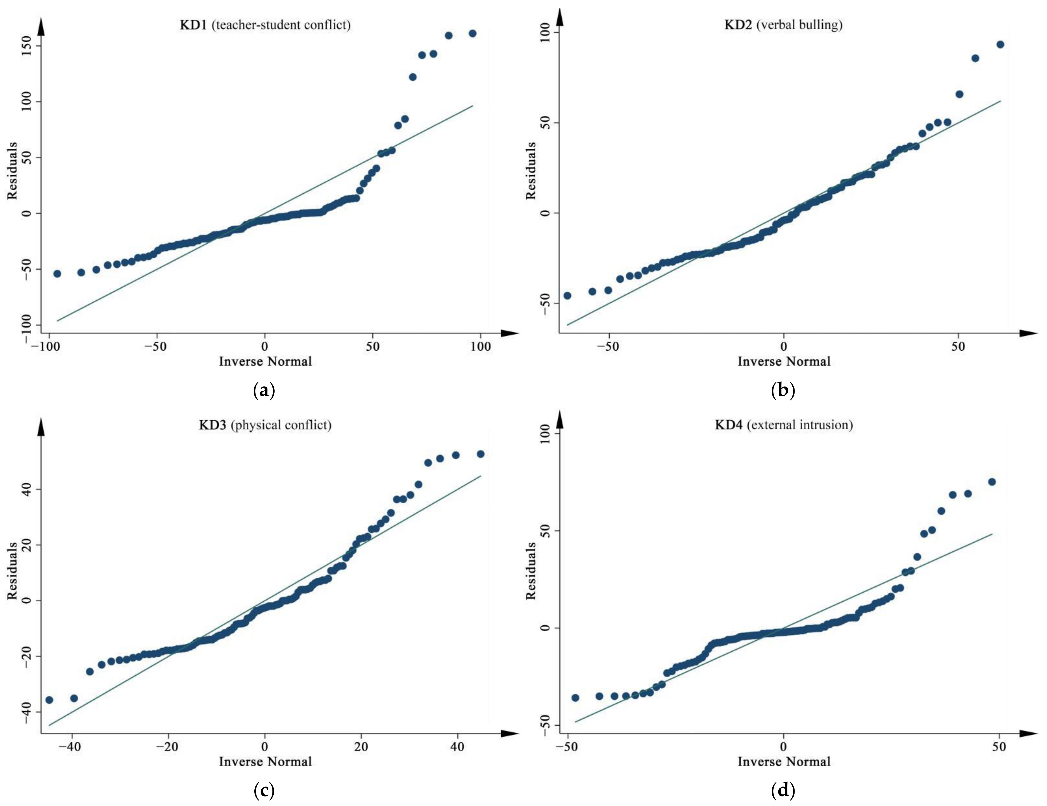
- Regression model checking: The validity, reliability, and generalizability of the model all should be tested in this step. Combined with previous literature [87,88,89], the difference between R2 and adjusted R2 could indicate the generalizability if the value was closer to zero. The Durbin–Watson statistic needed to be in the range of 1.0–3.0, and the maximum value of Cook’s Distance for all samples should be controlled to be less than 1.0 to demonstrate that the regression model had good reliability. It was also necessary to determine whether the regression residuals were approximately normally distributed based on normal Q–Q plots, with a better fit indicating a closer to normal distribution. As a complement, the results of the correlation and regression analysis needed to be combined to define the effective predictors of the regression model.
3. Results
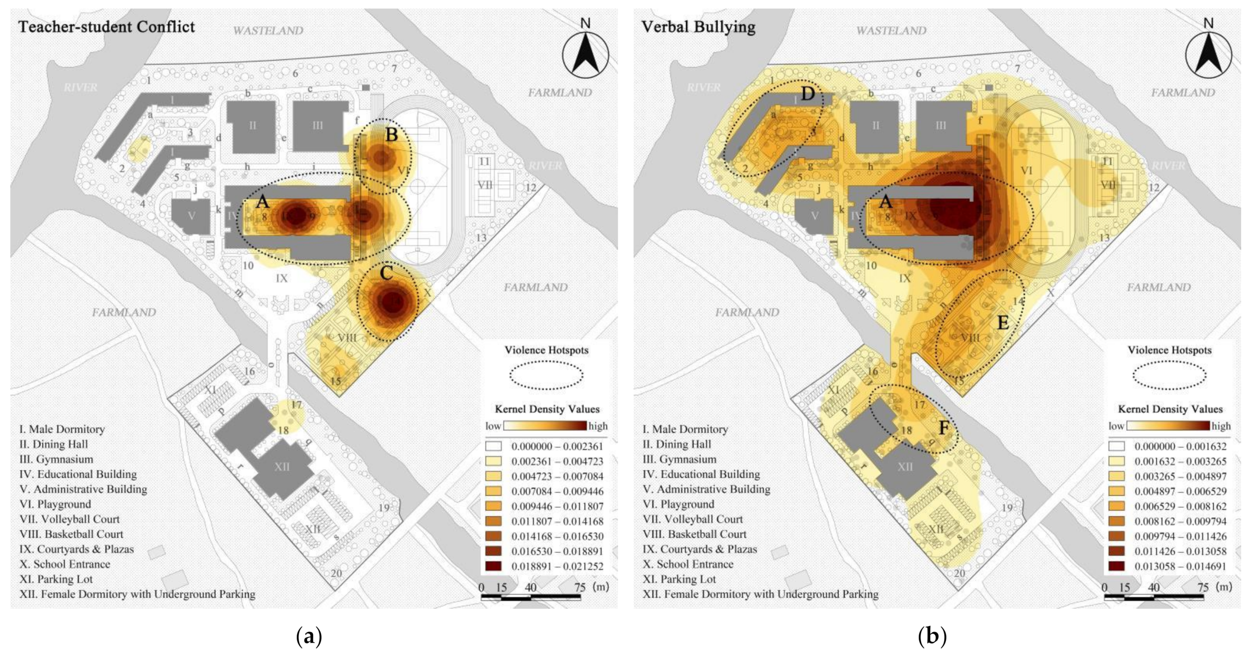
3.1. Kernel Density Distributions of Outdoor School Violence
3.2. Spatial Syntactic Graphs of the Outdoor Campus Environment
3.2.1. Spatial Configuration Graphs
3.2.2. Spatial Visibility Graphs
3.3. The Coupling Relationship between the OSVD and the OCE
3.3.1. Normal Distribution Test Results
3.3.2. Correlation Relationship
3.3.3. Regression Relationship and Models
3.3.4. Regression Model Checking Results
4. Discussion
5. Conclusions
Author Contributions
Funding
Institutional Review Board Statement
Informed Consent Statement
Data Availability Statement
Acknowledgments
Conflicts of Interest
Appendix A

| Level | Class | Subjects Number/Total Number (Stu.) | Sampling Ratio (%) | Sample Male Number/Sample Female Number (Stu.) | Mean Age |
|---|---|---|---|---|---|
| Freshman | 1 | 14/39 | 35.90 | 7/7 | 14.93 |
| 2 | 13/36 | 36.11 | 6/7 | 14.92 | |
| 3 | 13/38 | 34.21 | 6/7 | 14.85 | |
| 4 | 13/37 | 35.14 | 6/7 | 14.92 | |
| 5 | 13/37 | 35.14 | 6/7 | 15.00 | |
| 6 | 13/38 | 34.21 | 7/6 | 15.00 | |
| 7 | 13/37 | 35.14 | 7/6 | 14.92 | |
| 8 | 14/39 | 35.90 | 7/7 | 14.86 | |
| 9 | 13/37 | 35.14 | 7/6 | 15.00 | |
| 10 | 13/38 | 34.21 | 7/6 | 14.85 | |
| Sophomore | 1 | 13/36 | 36.11 | 6/7 | 15.92 |
| 2 | 12/35 | 34.29 | 6/6 | 15.92 | |
| 3 | 13/37 | 35.14 | 6/7 | 15.85 | |
| 4 | 12/35 | 34.29 | 6/6 | 16.00 | |
| 5 | 13/36 | 36.11 | 6/7 | 15.77 | |
| 6 | 12/34 | 35.29 | 6/6 | 15.92 | |
| 7 | 12/35 | 34.29 | 6/6 | 16.00 | |
| 8 | 13/36 | 36.11 | 7/6 | 15.92 | |
| 9 | 13/37 | 35.14 | 7/6 | 15.85 | |
| 10 | 12/35 | 34.29 | 6/6 | 15.83 | |
| 11 | 12/34 | 35.29 | 6/6 | 16.00 | |
| 12 | 13/37 | 35.14 | 7/6 | 15.85 | |
| 13 | 12/35 | 34.29 | 6/6 | 16.00 | |
| Senior | 1 | 14/40 | 35.00 | 7/7 | 16.93 |
| 2 | 14/40 | 35.00 | 7/7 | 16.86 | |
| 3 | 15/42 | 35.71 | 7/8 | 16.93 | |
| 4 | 13/38 | 34.21 | 6/7 | 16.92 |
| Dear Tested Subjects. Hello! Sincerely thank you for taking your valuable time to participate in our questionnaire activities. In order to fully protect your privacy, we guarantee that we will not disclose your personal information (including name, contact details, email address, etc.) in any form. | |||||
| Part One: Personal Information Statistics | |||||
| 1. What is your gender? | |||||
| A. Male | B. Female | ||||
| 2. What grade are you currently in? | |||||
| A. Senior year | B. Senior year | C. Senior year | |||
| 3. Where does your family live? | |||||
| A. Rural area | B. Suburban area | C. Urban area | |||
| 4. Are you a left-behind child? | |||||
| A. Yes | B. No | ||||
| Part Two: Outdoor School Violence Statistics | |||||
| 1. During your formative years, were you subjected to or did you inflict violence on others in school? (Please place a check mark in the matching blank box, multiple answers allowed) | |||||
| Cynicism from a teacher | ( ) | Refusal to allow others to participate in group activities | ( ) | ||
| Being physically punished by a teacher | ( ) | Exclusion of the same or opposite sex | ( ) | ||
| Insulting nicknames | ( ) | Kicking and punching others | ( ) | ||
| Isolating others | ( ) | Fighting and brawling | ( ) | ||
| Ridiculing others for being gender non-conforming | ( ) | Being intimidated or threatened by someone from outside the school | ( ) | ||
| Pushing or shoving someone on purpose | ( ) | Extortion of property by someone from outside the school | ( ) | ||
| Verbal threats | ( ) | Fighting with people from outside the school | ( ) | ||
| 2. To your knowledge, outdoor school violence at your school generally occurs mainly in (multiple choice)? | |||||
| Office entrance | ( ) | The way to school | ( ) | ||
| Classroom entrance | ( ) | School entrance | ( ) | ||
| School corridor | ( ) | Entertainment venues | ( ) | ||
| Playground | ( ) | Stairwell | ( ) | ||
| Area near the toilet | ( ) | Secluded grove | ( ) | ||
| Area around the dormitory | ( ) | ||||
| 3. To your knowledge, which type of abuser predominates in your school (multiple answers allowed)? | |||||
| Male | ( ) | Female | ( ) | ||
| Senior class | ( ) | Junior class | ( ) | ||
| Same class | ( ) | Others (teachers or external personnel) | ( ) | ||
| 4. To your knowledge, are there any teacher-student conflicts in your school? | |||||
| Yes | No | ||||
| 5. To your knowledge, please mark on the campus master plan below the spaces where you have experienced or observed outdoor school violence occurring. Please be careful and discreet. | |||||
| / | |||||
| Part Three: Current Environmental Assessment | |||||
| 1. The following questions ask how you feel about the current outdoor campus environment, please select the level of agreement based on your own experience. Please answer in an objective manner. | |||||
| Item | Strongly Agreed | Agreed | Neutral | Disagreed | Strongly Disagreed |
| Q1: Visual blind spots in landscape space | ( ) | ( ) | ( ) | ( ) | ( ) |
| Q2: Less road lamps or weak light | ( ) | ( ) | ( ) | ( ) | ( ) |
| Q3: Remote dormitory building | ( ) | ( ) | ( ) | ( ) | ( ) |
| Q4: Narrow school entrance and poor traffic order | ( ) | ( ) | ( ) | ( ) | ( ) |
| Q5: Hidden space blind spots on campus | ( ) | ( ) | ( ) | ( ) | ( ) |
| Q6: Lack of leisure facilities in public space | ( ) | ( ) | ( ) | ( ) | ( ) |
| Q7: Distant stadiums | ( ) | ( ) | ( ) | ( ) | ( ) |
| Q8: Low campus fence | ( ) | ( ) | ( ) | ( ) | ( ) |
| Q9: Lack of protective fence in dormitory | ( ) | ( ) | ( ) | ( ) | ( ) |
| Q10: Too dense and chaotic road network | ( ) | ( ) | ( ) | ( ) | ( ) |
| Q11: Confusing planning of school buildings | ( ) | ( ) | ( ) | ( ) | ( ) |
| Q12: Poorly managed green space | ( ) | ( ) | ( ) | ( ) | ( ) |
| Q13: Untimely litter removal | ( ) | ( ) | ( ) | ( ) | ( ) |
| Q14: Lack of security patrols at night | ( ) | ( ) | ( ) | ( ) | ( ) |
| Q15: Lack of security bulletin board | ( ) | ( ) | ( ) | ( ) | ( ) |
| Q16: Public facilities damaged | ( ) | ( ) | ( ) | ( ) | ( ) |
| The questionnaire section has been closed. Your responses will be counted anonymously and confidentiality will be guaranteed during the research process. Thank you very much for your support and cooperation with our team! | |||||
| Violence Types | Violence Activities | Perpetrators (%/Stu.) | Victims (%/Stu.) | Bystanders (%/Stu.) | Non-Experiencers (%/Stu.) |
|---|---|---|---|---|---|
| Teacher-student Conflict | Cynicism | 4.44/15 | 23.08/78 | 37.28/126 | 35.21/119 |
| Corporal punishment | 6.21/21 | 21.01/71 | 38.17/129 | 34.62/117 | |
| Verbal bullying | Insulting nickname | 15.98/54 | 13.02/44 | 41.42/140 | 29.59/100 |
| Isolating others | 15.09/51 | 11.54/39 | 40.53/137 | 32.84/111 | |
| Ridiculing others for the incompatibility of their personality with their gender | 7.10/24 | 5.92/20 | 42.90/145 | 44.08/149 | |
| Deliberately pushing others | 7.99/27 | 4.44/15 | 44.08/149 | 43.49/147 | |
| Verbal threat | 9.47/32 | 9.47/32 | 43.49/147 | 37.57/127 | |
| Refusing others to participate in collective activities | 7.10/24 | 4.44/15 | 43.49/147 | 44.97/152 | |
| Reject people of the same gender or opposite gender | 8.58/29 | 5.92/20 | 42.01/142 | 43.49/147 | |
| Physical conflict | Kicking and beating | 17.75/60 | 8.58/29 | 33.73/114 | 39.94/135 |
| Fighting | 6.67/23 | 5.33/18 | 52.89/178 | 35.21/119 | |
| External intrusion | Intimidation and threat | 1.48/5 | 9.17/31 | 39.94/135 | 46.15/156 |
| Blackmailing | 3.25/11 | 5.33/18 | 39.94/135 | 51.48/174 | |
| Affray | 0.59/2 | 2.66/9 | 27.51/93 | 69.23/234 |
| Item | Strongly Agreed (%/Stu.) | Agreed (%/Stu.) | Neutral (%/Stu.) | Disagreed (%/Stu.) | Strongly Disagreed (%/Stu.) |
|---|---|---|---|---|---|
| Q1: Visual blind spots in landscape space | 7.99/27 | 11.24/38 | 52.07/176 | 13.31/45 | 15.38/52 |
| Q2: Less road lamps or weak light | 5.03/17 | 12.13/41 | 45.56/154 | 17.75/60 | 19.53/66 |
| Q3: Remote dormitory building | 6.80/23 | 11.54/39 | 45.27/153 | 16.86/57 | 19.53/66 |
| Q4: Narrow school entrance and poor traffic order | 13.02/44 | 15.98/54 | 43.49/147 | 13.31/45 | 14.20/48 |
| Q5: Hidden space blind spots on campus | 5.92/20 | 13.02/44 | 42.60/144 | 21.60/73 | 16.86/57 |
| Q6: Lack of leisure facilities in public space | 5.03/17 | 12.43/42 | 42.60/144 | 19.53/66 | 20.41/69 |
| Q7: Distant stadiums | 8.58/29 | 11.54/39 | 42.01/142 | 17.16/58 | 17.75/60 |
| Q8: Low campus fence | 0.89/3 | 8.88/30 | 39.05/132 | 21.89/74 | 29.29/99 |
| Q9: Lack of protective fence in dormitory | 1.78/6 | 11.24/38 | 38.76/131 | 23.37/79 | 24.85/84 |
| Q10: Too dense and chaotic road network | 2.66/9 | 8.58/29 | 43.49/147 | 18.64/63 | 26.63/90 |
| Q11: Confusing planning of school buildings | 4.14/14 | 6.80/23 | 47.34/160 | 21.60/73 | 20.12/68 |
| Q12: Poorly managed green space | 0.89/3 | 5.33/18 | 41.72/141 | 21.30/72 | 30.77/104 |
| Q13: Untimely litter removal | 1.48/5 | 5.03/17 | 38.46/130 | 22.49/76 | 32.54/110 |
| Q14: Lack of security patrols at night | 4.73/16 | 10.65/36 | 42.90/145 | 21.30/72 | 20.41/69 |
| Q15: Lack of security bulletin board | 4.44/15 | 11.24/38 | 46.45/157 | 19.23/65 | 18.64/63 |
| Q16: Public facilities damaged | 1.78/6 | 9.76/33 | 45.86/155 | 18.64/63 | 23.96/81 |
Appendix B
| Item | Factor Loading | Communality | |
|---|---|---|---|
| Factor 1 | Factor 2 | ||
| Q1: Visual blind spots in landscape space | 0.720 | 0.530 | |
| Q2: Less road lamps or weak light | 0.797 | 0.691 | |
| Q3: Remote dormitory building | 0.766 | 0.631 | |
| Q5: Hidden space blind spots on campus | 0.500 | 0.480 | |
| Q6: Lack of leisure facilities in public space | 0.689 | 0.489 | |
| Q7: Distant stadiums | 0.640 | 0.460 | |
| Q8: Low campus fence | 0.779 | 0.692 | |
| Q9: Lack of protective fence in dormitory | 0.774 | 0.611 | |
| Q10: Too dense and chaotic road network | 0.668 | 0.522 | |
| Q11: Confusing planning of school buildings | 0.700 | 0.565 | |
| Q12: Poorly managed green space | 0.750 | 0.656 | |
| Q13: Untimely litter removal | 0.788 | 0.654 | |
| Q14: Lack of security patrols at night | 0.498 | 0.416 | |
| Q15: Lack of security bulletin board | 0.655 | 0.585 | |
| Q16: Public facilities damaged | 0.790 | 0.696 | |
References
- UNESCO. School Violence and Bullying: Global Status Report; UNESCO: Paris, France, 2017; p. 9. Available online: https://www.inclusive-education-in-action.org/resources/school-violence-and-bullying-global-status-report#:~:text=School%20Violence%20and%20Bullying%20Global%20Status%20Report%20The,schools%20to%20prevent%20and%20respond%20to%20the%20problem (accessed on 16 May 2022).
- Baker-Henningham, H.; Bowers, M.; Francis, T.; Vera-Hernández, M.; Walker, S.P. The Irie Classroom Toolbox, a universal violence-prevention teacher-training programme, in Jamaican preschools: A single-blind, cluster-randomised controlled trial. Lancet Glob. Health 2021, 9, e456–e468. [Google Scholar] [CrossRef]
- Riehm, K.E.; Mojtabai, R.; Adams, L.B.; Krueger, E.A.; Mattingly, D.T.; Nestadt, P.S.; Leventhal, A.M. Adolescents’ Concerns About School Violence or Shootings and Association With Depressive, Anxiety, and Panic Symptoms. JAMA Netw. Open 2021, 4, e2132131. [Google Scholar] [CrossRef] [PubMed]
- Xu, Z.; Fang, C. The Relationship between School Bullying and Subjective Well-Being: The Mediating Effect of School Belonging. Front. Psychol. 2021, 12, 725542. [Google Scholar] [CrossRef] [PubMed]
- Bochaver, A. School Bullying Experience and Current Well-Being among Students. Psikhologicheskaya Nauka I Obraz. 2021, 26, 17–27. [Google Scholar] [CrossRef]
- Ferrara, P.; Franceschini, G.; Namazova-Baranova, L.; Vural, M.; Mestrovic, J.; Nigri, L.; Giardino, I.; Pop, T.L.; Sacco, M.; Pettoello-Mantovani, M. Lifelong Negative Influence of School Violence on Children. J. Pediatr. 2019, 215, 287–288. [Google Scholar] [CrossRef] [PubMed] [Green Version]
- Luo, X.; Zheng, R.; Xiao, P.; Xie, X.; Liu, Q.; Zhu, K.; Wu, X.; Xiang, Z.; Song, R. Relationship between school bullying and mental health status of adolescent students in China: A nationwide cross-sectional study. Asian J. Psychiatry 2022, 70, 103043. [Google Scholar] [CrossRef]
- UNESCO. School Violence and Bullying: Global Status and Trends, Drivers and Consequences; UNESCO: Paris, France, 2018; pp. 4–7. Available online: http://www.infocoponline.es/pdf/BULLYING.pdf (accessed on 16 May 2022).
- Ministry of Education, PRC. National Statistical Bulletin on the Development of Education in 2017. Available online: http://www.moe.gov.cn/jyb_sjzl/sjzl_fztjgb/201807/t20180719_343508.html (accessed on 15 January 2022).
- Fu, W.; Zhou, W.; Li, W.; Chen, A. Survey Claims 32.4% Incidence of Bullying in Schools: Vulnerable Groups More Likely to Be Bullied. Available online: https://share.gmw.cn/edu/2021-11/01/content_1302660247.htm (accessed on 16 May 2022).
- Soonjung, K.; Hayoung, K. Exploring the Educational Possibility of Preventing School Violence by Cultural Transition: Reflecting upon school violence through the objectification phenomenon and revisiting the value of peace, human right, and relationship. J. Korean Educ. 2021, 48, 63–84. [Google Scholar] [CrossRef]
- Ilona, T.; Saulius, S.; Aurelijus, Z.; Aleksandras, A. Examining the Relations among Extraversion, Neuroticism, and School Bullying among Lithuanian Adolescents. Eur. J. Contemp. Educ. 2021, 10, 476–484. [Google Scholar] [CrossRef]
- Zhang, Y.; Li, Z.; Tan, Y.; Zhang, X.; Zhao, Q.; Chen, X. The Influence of Personality Traits on School Bullying: A Moderated Mediation Model. Front. Psychol. 2021, 12, 650070. [Google Scholar] [CrossRef]
- Romeiro, J.S.; Corrêa, M.M.; Pazó, R.; Leite, F.M.C.; Cade, N.V. Physical violence and associated factors in participants of the National Student Health Survey (NSHS). Cienc. Saude Coletiva 2021, 26, 611–624. [Google Scholar] [CrossRef]
- Buhaș, C.L.; Judea-Pusta, C.; Buhaș, B.A.; Bungau, S.; Judea, A.S.; Sava, C.; Popa, V.C.; Cioca, G.; Tit, D.M. Physical, Psychological and Sexual Abuse of the Minor in the Families from the Northwestern Region of Romania- Social and Medical Forensics. Iran. J. Public Health 2021, 50, 121–129. [Google Scholar] [CrossRef]
- Hultin, H.; Ferrer-Wreder, L.; Engström, K.; Andersson, F.; Galanti, M.R. The Importance of Pedagogical and Social School Climate to Bullying: A Cross-Sectional Multilevel Study of 94 Swedish Schools. J. Sch. Health 2021, 91, 111–124. [Google Scholar] [CrossRef]
- Reisen, A.; Leite, F.M.C.; Neto, E.T.D.S. Association between social capital and bullying among adolescents aged between 15 and 19: Relations between the school and social environment. Cienc. Saude Coletiva 2021, 26, 4919–4932. [Google Scholar] [CrossRef]
- Duque, E.; Carbonell, S.; de Botton, L.; Roca-Campos, E. Creating Learning Environments Free of Violence in Special Education Through the Dialogic Model of Prevention and Resolution of Conflicts. Front. Psychol. 2021, 12, 662831. [Google Scholar] [CrossRef]
- Shik, J.H. A Drama Therapy Program to Improve Spatial Awareness for Treating School Violence: Focusing on the Fairy Tale <The Ugly Duckling>. J. Drama Art Ther. 2021, 15, 1–33. [Google Scholar] [CrossRef]
- Oscós-Sánchez, M.; Lesser, J.; Oscós-Flores, L.D.; Pineda, D.; Araujo, Y.; Franklin, B.; Hernández, J.A.; Hernández, S.; Vidales, A. The Effects of Two Community-Based Participatory Action Research Programs on Violence Outside of and in School Among Adolescents and Young Adults in a Latino Community. J. Adolesc. Health 2020, 68, 370–377. [Google Scholar] [CrossRef]
- Glubwila, S.; Sripa, K.; Thummaphan, P. The model of collaboration integration for preventing and solving the problem of youth violence in educational settings. Curr. Psychol. 2021, 1–10. [Google Scholar] [CrossRef]
- Zeng, M.; Sun, W.; Mao, Y.; Liang, Y.; Wu, Q. Study and enlightenment on prevention measures of overseas campus crime. Urban Des. 2018, 5, 64–73. (In Chinese) [Google Scholar] [CrossRef]
- Foody, M.; Challenor, L.; Murphyy, H.; Norman, J.O. The Anti-Bullying Procedures for Primary and Post-Primary Schools in Ireland: What Has Been Achieved and What Needs to be done. Bild. Und Erzieh. 2018, 71, 88–97. [Google Scholar] [CrossRef]
- Kalichman, S.C.; Brosig, C.L. Mandatory Child Abuse Reporting Laws: Issues and Implications for Policy. Law Policy 1992, 14, 153–168. [Google Scholar] [CrossRef]
- Kim, N. The Police Action against School Violence in Korea. Ph.D. Thesis, Tsinghua University, Beijing, China, 2015. Available online: https://kns.cnki.net/kcms/detail/detail.aspx?dbcode=CMFD&dbname=CMFD201602&filename=1016713201.nh&uniplatform=NZKPT&v=gHRM9V6EneLWiTvU-V3EQk5owmiyE6cT2VjFElj79XS08dd4_KYizSjB9S1EsMyC (accessed on 16 May 2022).
- Sairanen, L.; Pfeffer, K. Self-reported handling of bullying among junior high school teachers in Finland. Sch. Psychol. Int. 2011, 32, 330–344. [Google Scholar] [CrossRef]
- Kim, Y.O. A Study on the Regional Professional Program for the School Violence Prevention. Korean Assoc. Police Sci. Rev. 2021, 23, 175–202. [Google Scholar] [CrossRef]
- Sullivan, T.N.; Farrell, A.D.; Sutherland, K.S.; Behrhorst, K.L.; Garthe, R.C.; Greene, A. Evaluation of the Olweus Bullying Prevention Program in US Urban Middle Schools Using a Multiple Baseline Experimental Design. Prev. Sci. 2021, 22, 1134–1146. [Google Scholar] [CrossRef]
- Bradshaw, C.P.; Waasdorp, T.E.; Debnam, K.J.; Johnson, S.L. Measuring school climate in high schools: A focus on safety, engagement, and the environment. J. Sch. Health 2014, 84, 593–604. [Google Scholar] [CrossRef]
- Lamoreaux, D.J.; Sulkowski, M.L. Crime Prevention through Environmental Design in schools: Students’ perceptions of safety and psychological comfort. Psychol. Sch. 2021, 58, 475–493. [Google Scholar] [CrossRef]
- Lu, P.; Chen, D.; Li, Y.; Wang, X.; Yu, S. Agent-Based Model of Mass Campus Shooting: Comparing Hiding and Moving of Civilians. IEEE Trans. Comput. Soc. Syst. 2022, 1–10. [Google Scholar] [CrossRef]
- Aggarwal, J.; Eitland, E.S.; Gonzalez, L.N.; Greenberg, P.; Kaplun, E.; Sahili, S. Built Environment Attributes and Preparedness for Potential Gun Violence at Secondary Schools. J. Environ. Health 2021, 84, 8–16. Available online: https://www.neha.org/node/62303 (accessed on 16 May 2022).
- Ma, N.; Ma, S.; Li, S.; Ma, S.; Pan, X.; Sun, G. The Study of Spatial Safety and Social Psychological Health Features of Deaf Children and Children with an Intellectual Disability in the Public School Environment Based on the Visual Access and Exposure (VAE) Model. Int. J. Environ. Res. Public Health 2021, 18, 4322. [Google Scholar] [CrossRef] [PubMed]
- Cozens, P.M.; Saville, G.; Hillier, D. Crime prevention through environmental design (CPTED): A review and modern bibliography. Prop. Manag. 2005, 23, 328–356. [Google Scholar] [CrossRef] [Green Version]
- Armitage, R. Burglars’ take on crime prevention through environmental design (CPTED): Reconsidering the relevance from an offender perspective. Secur. J. 2018, 31, 285–304. [Google Scholar] [CrossRef] [Green Version]
- Mao, Y.; Yin, L.; Zeng, M.; Ding, J.; Song, Y. Review of Empirical Studies on Relationship between Street Environment and Crime. J. Plan. Lit. 2021, 36, 187–202. [Google Scholar] [CrossRef]
- Tuba, K.; Colpan, E.N. Design Guidelines for Urban Safety. J. Plan. 2022, 32, 162–173. [Google Scholar] [CrossRef]
- Jacobs, J. The Death and Life of Great American Cities; Vintage Books: New York, NY, USA, 1961. [Google Scholar] [CrossRef]
- Jeffery, C.R. Crime Prevention through Environmental Design; Sage Publications: Beverly Hills, CA, USA, 1971. [Google Scholar] [CrossRef]
- Newman, O. Defensible Space: Crime Prevention through Urban Design; Macmillan: New York, NY, USA, 1972. [Google Scholar] [CrossRef]
- Cozens, P.; Love, T. A Review and Current Status of Crime Prevention through Environmental Design (CPTED). J. Plan. Lit. 2015, 30, 393–412. [Google Scholar] [CrossRef]
- Liu, C. Environment Redesigned for Crime Prevention with CPTED Strategies: A Case Study of Typical Chinese Community. Appl. Mech. Mater. 2014, 3309, 805–810. [Google Scholar] [CrossRef]
- Rupp, L.A.; Zimmerman, M.A.; Sly, K.W.; Reischl, T.M.; Thulin, E.J.; Wyatt, T.A.; Stock, J. Community-Engaged Neighborhood Revitalization and Empowerment: Busy Streets Theory in Action. Am. J. Community Psychol. 2020, 65, 90–106. [Google Scholar] [CrossRef]
- Curtis-Ham, S.; Cantal, C.; Gravitas Research Ltd. Locks, lights, and lines of sight: An RCT evaluating the impact of a CPTED intervention on repeat burglary victimisation. J. Exp. Criminol. 2022, 1–28. [Google Scholar] [CrossRef]
- Surette, R.; Stephenson, M. Expectations versus effects regarding police surveillance cameras in a municipal park. Crime Prev. Community Saf. 2019, 21, 22–41. [Google Scholar] [CrossRef]
- Cho, M.-G.; Park, C.; Jang, J.-I. The Effects of Urban Park and Vegetation on Crime in Seoul and Its Planning Implication to CPTED. J. Korean Inst. Landsc. Archit. 2018, 46, 27–35. [Google Scholar] [CrossRef] [Green Version]
- Yeom, S.-J.; Hong, Y.-S. A Case Study on Application of CPTED of Park Development Guidelines. J. Environ. Sci. Int. 2017, 26, 97–107. [Google Scholar] [CrossRef]
- Zhang, Y.; Yang, F.; Wang, M. Investigation of Urban Park Crime Prevention Based on CPTED Theory and Space Syntax Taking People’s Park and Zijingshan Park in Zhengzhou as Examples. J. Southwest Univ. Nat. Sci. Ed. 2022, 44, 202–212. [Google Scholar] [CrossRef]
- Su, J.; Yin, W.; Zhang, R.; Zhao, X.; Chinkam, O.N.; Zhang, H.; Li, F.; Kang, L. A Multi-source Data Based Analysis Framework for Urban Greenway Safety. Teh. Vjesn.-Tech. Gaz. 2021, 28, 193–202. [Google Scholar] [CrossRef]
- Erman, A. Evaluation of Crime Prevention Theories through Environmental Design in Urban Renewal: A Case Study of Ankara—The Vicinity of Haci Bayram Mosque. ICONARP Int. J. Archit. Plan. 2021, 9, 896–918. [Google Scholar] [CrossRef]
- Kang, H. Effect of the Local Community’s Perception of Urban Regeneration and CPTED on Safety Life Satisfaction. Korean Secur. J. 2022, 70, 267–292. [Google Scholar] [CrossRef]
- Yang, M.-Y.; Cho, J.-H. A Study of CPTED Design Color to Urban Regeneration in Alley Street of Waterfront—Focused on Bongsan Village, Bongrae 2-dong, Yeongdo-gu, Busan. J. Korea Soc. Color Stud. 2021, 35, 44–54. [Google Scholar] [CrossRef]
- Badiora, A.I.; Dada, O.T.; Adebara, T.M. Correlates of crime and environmental design in a Nigerian international tourist attraction site. J. Outdoor Recreat. Tour. 2021, 35, 100392. [Google Scholar] [CrossRef]
- Sun, Y.N. The Research on the Design Method of Crime Prevention in Hospital Buildings. Master’s Thesis, Beijing University of Civil Engineering and Architecture, Beijing, China, 2017. Available online: https://kns.cnki.net/kcms/detail/detail.aspx?dbcode=CMFD&dbname=CMFD201801&filename=1017169696.nh&uniplatform=NZKPT&v=lndDiwhdBjD3B2HWVPufFgZaBvBWj_Wh2ppH6H1y93B-KHAsnwjRAjySO2TyPcvQ (accessed on 16 May 2022).
- El-Hadedy, N.; El-Husseiny, M. Evidence-Based Design for Workplace Violence Prevention in Emergency Departments Utilizing CPTED and Space Syntax Analyses. HERD 2021, 15, 19375867211042902. [Google Scholar] [CrossRef] [PubMed]
- Hyeji, R. A Study on the Physical Environmental Factors Causing Crime Fear of College Towns in Urban and Rural Complex Areas—Focusing on Hongseong-eup, Hongseong-gun. J. Korea Intitute Spat. Des. 2021, 16, 169–178. [Google Scholar] [CrossRef]
- Jones, F.; Sloboden, J. Jacksonville, Florida, Transportation Authority’s Mobility Corridors: Improving Transit System Performance through Enhanced Safety and Urban Design. Transp. Res. Rec. 2017, 2651, 118–126. [Google Scholar] [CrossRef]
- Kim, W. A Study on the Effects of CPTED on Social Interaction among Students—Focused on the Environment of University Dormitory. J. Archit. Inst. Korea 2021, 37, 77–84. [Google Scholar] [CrossRef]
- He, L.; Kwan, S.-H. A Study on the 3rd Generation CPTED Process through Double Diamond. J. Korea Contents Assoc. 2022, 22, 207–221. [Google Scholar] [CrossRef]
- Gouveia, F.; Sani, A.; Guerreiro, M.; Azevedo, V.; Santos, H.; Nunes, L.M. Mapping CPTED parameters with the LookCrim application. Crime Prev. Community Saf. 2021, 23, 252–263. [Google Scholar] [CrossRef]
- Azevedo, V.; Maia, R.L.; Guerreiro, M.J.; Oliveira, G.; Sani, A.; Caridade, S.; Dinis, M.A.P.; Estrada, R.; Paulo, D.; Magalhães, M.; et al. Looking at crime-communities and physical spaces: A curated dataset. Data Brief 2021, 39, 107560. [Google Scholar] [CrossRef]
- Wilcox, P.; Quisenberry, N.; Jones, S. The Built Environment and Community Crime Risk Interpretation. J. Res. Crime Delinq. 2003, 40, 322–345. [Google Scholar] [CrossRef]
- Johnson, S.D.; Bowers, K.J. Permeability and Burglary Risk: Are Cul-de-Sacs Safer? J. Quant. Criminol. 2010, 26, 89–111. [Google Scholar] [CrossRef]
- Feng, J.; Huang, L.; Dong, Y.; Song, L. Research on the spatia-temporal characteristics and mechanism of urban crime:A case study of property crime in Beijing. Acta Geogr. Sin. 2012, 67, 1645–1656. (In Chinese) [Google Scholar] [CrossRef]
- He, R.; Xu, Y.; Jiang, S. Applications of GIS in Public Security Agencies in China. Asian J. Criminol. 2022, 17, 213–235. [Google Scholar] [CrossRef]
- Leydesdorff, L. Patent classifications as indicators of intellectual organization. J. Am. Soc. Inf. Sci. Technol. 2008, 59, 1582–1597. [Google Scholar] [CrossRef] [Green Version]
- Mehrotra, D.; Kumar, M.; Singh, S.N.; Sukhija, K. Spatial and temporal trends reveal: Hotspot identification of crimes using machine learning approach. Int. J. Comput. Sci. Eng. 2022, 25, 174–185. [Google Scholar] [CrossRef]
- Abd El AZIZ, N.A. Space Syntax as a Tool to Measure Safety in Small Urban Parks: A Case Study of Rod El Farag Park in Cairo, Egypt. Landsc. Archit. Front. 2020, 8, 42–59. [Google Scholar] [CrossRef]
- Matijosaitiene, I. Combination of CPTED and space syntax for the analysis of crime. Saf. Communities 2016, 15, 49–62. [Google Scholar] [CrossRef]
- Hillier, B.; Hanson, J. The Social Logic of Space; Cambridge University Press: Cambridge, UK, 1984. [Google Scholar] [CrossRef]
- Sherman, S.A. Policing the Campus: Police Communications and near-Campus Development across Atlanta’s University Communities. Plan. Theory Pract. 2022. [Google Scholar] [CrossRef]
- Ministry of Education, PRC. National Statistical Bulletin on the Development of Education in 2011. Available online: http://www.moe.gov.cn/srcsite/A03/s180/moe_633/201208/t20120830_141305.html (accessed on 17 January 2022).
- Li, H.M. A Study on the Strategy of Prevention and Control of Bullying in the Rural Boarding Schools: Case of S Township Middle School in Henan Province. Master’s Thesis, Southwest University, Chongqing, China, 2018. Available online: https://kns.cnki.net/kcms/detail/detail.aspx?dbcode=CMFD&dbname=CMFD201901&filename=1018857455.nh&uniplatform=NZKPT&v=0i2Rp6Jh6_rgGOwloADlN5vF8-4YwFSD-wZUfoTvWs3bOCxYg4pn4lveodjxROIG (accessed on 10 June 2022).
- William, G.C. Sampling Techniques, 3rd ed.; Wiley Publication: Hoboken, NJ, USA, 1977; Available online: https://www.wiley.com/en-in/Sampling+Techniques%2C+3rd+Edition-p-9780471162407 (accessed on 16 May 2022).
- Huang, D. Perceived Safety Evaluation and Design Strategy of Guangzhou Higher Education Mega Center Based on Crime Prevention through Environmental Design. Master’s Thesis, South China University of Technology, Guangzhou, China, 2020. [Google Scholar] [CrossRef]
- Liu, H.; Zhang, Z.; Ma, X.; Lu, W.; Li, D.; Kojima, S. Optimization Analysis of the Residential Window-to-Wall Ratio Based on Numerical Calculation of Energy Consumption in the Hot-Summer and Cold-Winter Zone of China. Sustainability 2021, 13, 6138. [Google Scholar] [CrossRef]
- Gopalakrishnan, R.; Guevara, C.A.; Ben-Akiva, M. Combining multiple imputation and control function methods to deal with missing data and endogeneity in discrete-choice models. Transp. Res. Part B Methodol. 2020, 142, 45–57. [Google Scholar] [CrossRef]
- Wang, P. A Survey of Bullying in Rural Junior High Schools: From the Perspective of Students. Master’s Thesis, Guangxi Normal University, Guilin, China, 2021. [Google Scholar] [CrossRef]
- Wamg, H. Research on the Status and Prevention of School Bullying in Rural Junior Middle School. Master’s Thesis, Southeast University, Nanjing, China, 2020. [Google Scholar] [CrossRef]
- Jiaping, Y. The Current Situation and Countermeasures of Bullying in Private Boarding Junior Middle Schools from the Perspective of Social Ecosystem: Taking a Middle School. Master’s Thesis, South China University of Technology, Guangzhou, China, 2020. [Google Scholar] [CrossRef]
- López-Castedo, A.; García, D.; José, D.A.; Roales, E.A. Expressions of school violence in adolescence. Psicothema 2018, 30, 395–400. [Google Scholar] [CrossRef]
- Kearney, C.A. School absenteeism and school refusal behavior in youth: A contemporary review. Clin. Psychol. Rev. 2008, 28, 451–471. [Google Scholar] [CrossRef]
- Cheng, J.; Sun, L.; Wang, T.; Xu, F.; Sun, L. The coupling relationship between crime distribution and urban environment in Lanzhou city center. Sci. Surv. Mapp. 2021, 46, 167–174. (In Chinese) [Google Scholar] [CrossRef]
- Hillier, B. Space is the Machine: A Configurationally Theory of Architecture; Cambridge University Press: Cambridge, UK, 1996; Available online: https://discovery.ucl.ac.uk/id/eprint/3848/1/SpaceIsTheMachine_Part1.pdf#:~:text=Space%20is%20the%20Machine%20was%20first%20published%20in,outline%20a%20configurational%20theory%20of%20architecture%20and%20urbanism (accessed on 16 May 2022).
- Alalouch, C.; Al-Hajri, S.; Naser, A.; Al Hinai, A. The Impact of Space Syntax Spatial Attributes on Urban Land Use in Muscat: Implications for Urban Sustainability. Sustain. Cities Soc. 2019, 46, 101417. [Google Scholar] [CrossRef]
- Field, A. Discovering Statistics Using SPSS, 3rd ed.; SAGE Publication: London, UK, 2009; Available online: http://senas.lnb.lt/stotisFiles/uploadedAttachments/9_Discovering_statistics_using_SPSS201012510426.pdf (accessed on 16 May 2022).
- Bowerman, B.L.; O’Connell, R.T. Linear Statistical Models: An Applied Approach, 2nd ed.; Duxbury: Belmont, TN, USA, 2000; Available online: https://books.google.com/books/about/Linear_Statistical_Models.html?id=O2gCAAAACAAJ#:~:text=The%20focus%20of%20%EE%80%80Linear%20Statistical%20Models%3A%20An%20Applied,accessible%20even%20to%20those%20with%20limited%20%EE%80%80statistical%EE%80%81%20experience (accessed on 16 May 2022).
- Ralph, J. Linear Statistical Models: An Applied Approach. Technometrics 2012, 29, 237–238. [Google Scholar] [CrossRef]
- Chatterjee, S.; Hadi, A.S. Regression Analysis by Example; Wiley-Interscience Publication: Hoboken, NJ, USA, 2006. [Google Scholar] [CrossRef]
- Wang, M. Research on Web-Based Spatial Data Grab and Evaluation. Ph.D. Thesis, Wuhan University, Wuhan, China, 2013. Available online: https://kns.cnki.net/kcms/detail/detail.aspx?dbcode=CDFD&dbname=CDFD1214&filename=1013209390.nh&uniplatform=NZKPT&v=iPGGZ4TNJ7aP5tatbjoBJXzejBDT0l0huG1zYFloI_d1cDKlR8-Hvae0E8TmtnMl (accessed on 16 May 2022).
- Weisberg, S. Applied Linear Regression, 3rd ed.; Wiley Publication: Hoboken, NJ, USA, 2005. [Google Scholar] [CrossRef]
- Moon, B.; McCluskey, J. School-Based Victimization of Teachers in Korea: Focusing on Individual and School Characteristics. J. Interpers. Violence 2016, 31, 1340–1361. [Google Scholar] [CrossRef]
- Alves, A.G.; Cesar, F.C.R.; Barbosa, M.A.; Oliveira, L.M.D.A.C.; da Silva, E.A.S.; Rodríguez-Martín, D. Dimensions of student violence against the teacher. Cienc. Saude Coletiva 2022, 27, 1027–1038. [Google Scholar] [CrossRef]
- Jia, Y. Research on the Crime Prevention of Aggressive School Violence Based on CPTED Theory. Master’s Thesis, Xinyang Normal University, Xinyang, China, 2021. [Google Scholar] [CrossRef]
- Kweon, J. A Study on the Architectural Planning of Elementary School for Violence Prevention—Through Analyzing Space Composition and Visibility Characteristics of Elementary Schools in Daegu City. J. Reg. Assoc. Archit. Inst. Korea 2018, 10, 47–56. Available online: https://www.kci.go.kr/kciportal/ci/sereArticleSearch/ciSereArtiView.kci?sereArticleSearchBean.artiId=ART001264911 (accessed on 16 May 2022).
- Ju, M.-O.; Lee, C.-H. School Territories and Complementary Strategies of CPTED for Each School Territory. J. Community Saf. Secur. Environ. Des. 2017, 8, 179–216. [Google Scholar] [CrossRef]
- Charles, C.L. Collective efficacy and the built environment. Criminology 2022, 60, 370–396. [Google Scholar] [CrossRef]
- Jiang, D.; Qiu, B. Comparison of effects of spatial anticrime in open communities in China. J. Asian Arch. Build. Eng. 2020, 20, 237–247. [Google Scholar] [CrossRef]
- Hu, H.; Huang, X.; Suhaim, M.A.; Zhang, H. Comparison of compression estimations under the penalty functions of different violent crimes on campus through deep learning and linear spatial autoregressive models. Appl. Math. Nonlinear Sci. 2021. [Google Scholar] [CrossRef]
- Qiao, Y.; Xing, Y.; Duan, J.; Bai, C.; Pan, Y.; Cui, Y.; Kong, J. Prevalence and associated factors of school physical violence behaviors among middle school students in Beijing. Chin. J. Epidemiol. 2010, 31, 510–512. Available online: https://kns.cnki.net/kcms/detail/detail.aspx?dbcode=CJFD&dbname=CJFDZHYX&filename=ZHLX201005014&uniplatform=NZKPT&v=0MMKBU2dhWm82sqOXphURLkuW-NuCxWPKcNvvd18yfm5uf-QWRXN8QBqXtT0YuRQ (accessed on 16 May 2022). (In Chinese).
- Wang, H.; Tang, J.; Dill, S.-E.; Xiao, J.; Boswell, M.; Cousineau, C.; Rozelle, S. Bullying Victims in Rural Primary Schools: Prevalence, Correlates, and Consequences. Int. J. Environ. Res. Public Health 2022, 19, 765. [Google Scholar] [CrossRef]
- Sadjadi, M.; Blanchard, L.; Brülle, R.; Bonell, C. Barriers and facilitators to the implementation of Health-Promoting School programmes targeting bullying and violence: A systematic review. Health Educ. Res. 2021, 36, 581–599. [Google Scholar] [CrossRef]
- Evans, D.; Butterworth, R.; Law, G.U. Understanding associations between perceptions of student behaviour, conflict representations in the teacher-student relationship and teachers’ emotional experiences. Teach. Teach. Educ. 2019, 82, 55–68. [Google Scholar] [CrossRef]
- Scharpf, F.; Kirika, A.; Masath, F.B.; Mkinga, G.; Ssenyonga, J.; Nyarko-Tetteh, E.; Nkuba, M.; Karikari, A.K.; Hecker, T. Reducing physical and emotional violence by teachers using the intervention Interaction Competencies with Children—For Teachers (ICC-T): Study protocol of a multi-country cluster randomized controlled trial in Ghana, Tanzania, and Uganda. BMC Public Health 2021, 21, 1930. [Google Scholar] [CrossRef]
- Hyoen, K.N.; JihooA, K. Study on Quantitative CPTED Guideline Selection Model for Public Street Considering Spatial Characteristics of Juvenile Crimes in School Surroundings. J. Digit. Des. 2016, 16, 328–356. [Google Scholar]
- Wahab, A.A.; Sakip, S.R.M. Mapping Isolated Places in School in Concurrence with Bullying Possibility Elements. Environ. Behav. Proc. J. 2020, 4, 359–366. [Google Scholar] [CrossRef]
- Shariati, A. Crime prevention through environmental design (CPTED) and its potential for campus safety: A qualitative study. Secur. J. 2021. [Google Scholar] [CrossRef]
- Tomita, M.; Tago, T.; Ohuchi, H. Correlation between Color Composition of District, Environment Recognition and Behavioral Characteristics in Cityscape: Case study in Ginza and Harajuku area (Environmental Engineering). AIJ J. Technol. Des. 2003, 9, 279–282. [Google Scholar] [CrossRef] [Green Version]
- Braun, C.C.; Greeno, B.; Silver, N.C. Differences in Behavioral Compliance as a Function of Warning Color. Proc. Hum. Factors Ergon. Soc. Annu. Meet. 1994, 38, 379–383. [Google Scholar] [CrossRef]
- Ross, S. Introduction to Probability Models, 12th ed.; Academic Press: Pittsburgh, PA, USA, 2019; Available online: https://www.elsevier.com/books/introduction-to-probability-models/ross/978-0-12-814346-9 (accessed on 10 June 2022).
- Chung, R.H.; Kim, B.S.; Abreu, J.M. Asian American multidimensional acculturation scale: Development, factor analysis, reliability, and validity. Cult. Divers. Ethn. Minor. Psychol. 2004, 10, 66–80. [Google Scholar] [CrossRef] [PubMed] [Green Version]
- Yoon, E.; Langrehr, K.; Ong, L.Z. Content Analysis of Acculturation Research in Counseling and Counseling Psychology: A 22-Year Review. J. Couns. Psychol. 2010, 58, 83–96. [Google Scholar] [CrossRef] [PubMed] [Green Version]


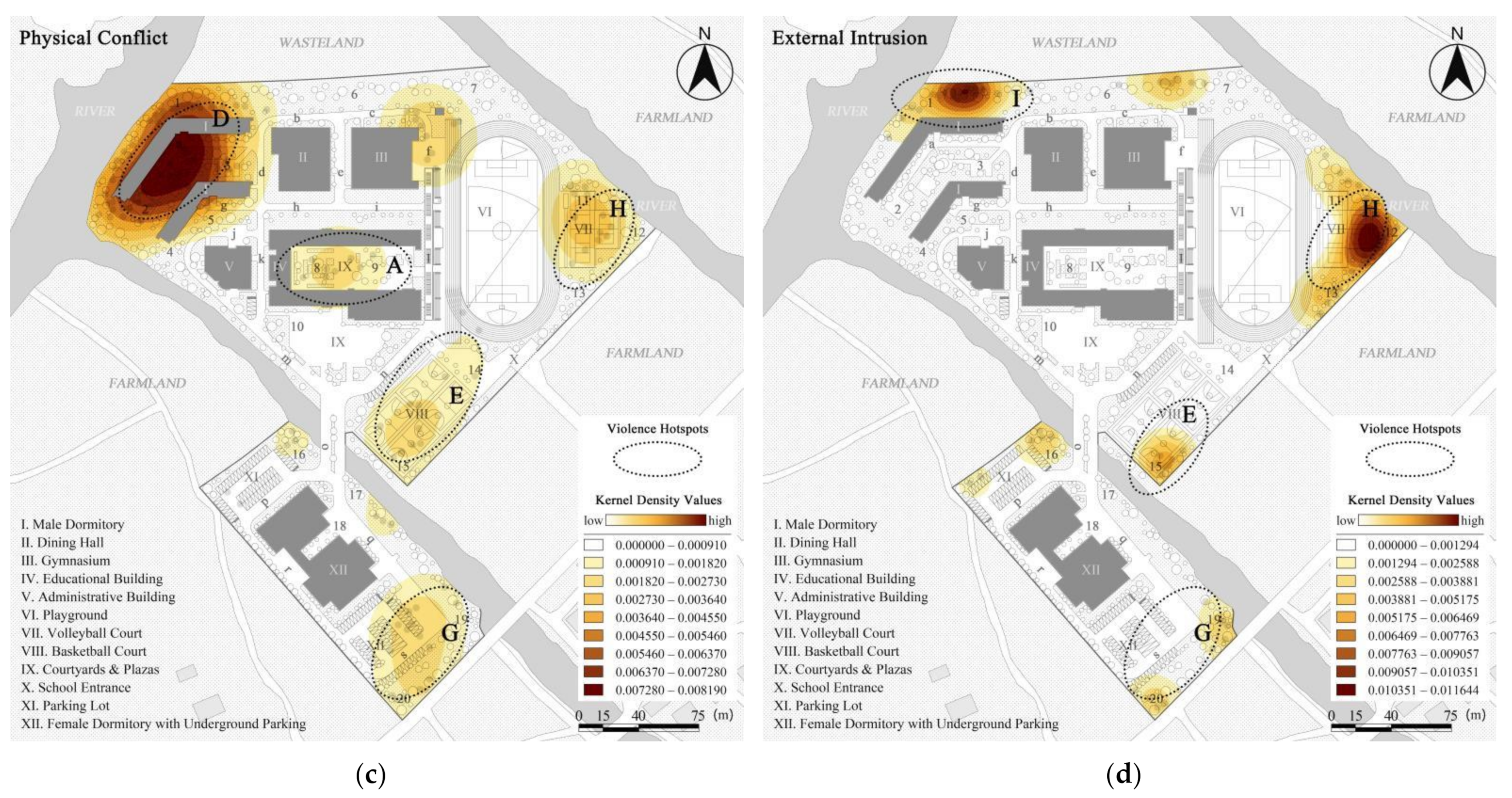


| Violence Types | Violence Activities | Number | Total Percentage (%) | Spatial Distribution Map |
|---|---|---|---|---|
| Teacher-student conflict | Cynicism | 93 | 22.64 |  |
| Corporal punishment | 92 | |||
| Verbal bullying | Insulting nickname | 98 | 52.14 |  |
| Isolating others | 90 | |||
| Ridiculing others for the incompatibility of their personality with their gender | 44 | |||
| Deliberately pushing others | 42 | |||
| Verbal threat | 64 | |||
| Refusing others to participate in collective activities | 39 | |||
| Reject people of the same gender or opposite gender | 49 | |||
| Physical conflict | Kicking and beating | 89 | 15.92 |  |
| Fighting | 41 | |||
| External intrusion | Intimidation and threat | 36 | 9.30 |  |
| Blackmailing | 29 | |||
| Affray | 11 |
| Object | Type | Trunk Height | Canopy Size | Opacity in Summer | Opacity in Winter |
|---|---|---|---|---|---|
| Cinnamomum camphora | Evergreen tree | Medium | Large | High | High |
| Ligustrum lucidum | Evergreen tree | High | Large | Low | Low |
| Ginkgo biloba | Deciduous tree | Medium | Small | High | Low |
| Metasequoia | Deciduous tree | Medium | Small | High | Low |
| Osmanthus fragrans | Evergreen tree | Medium | Medium | High | High |
| Magnolia grandiflora | Evergreen tree | High | Large | Low | Low |
| Camellia japonica L. | Evergreen tree | Low | Medium | High | High |
| Liquidambar formosana Hance | Deciduous tree | Low | Medium | High | Low |
| Liriodendron chinense | Deciduous tree | High | Large | Low | Low |
| Punica granatum L. | Deciduous tree | Low | Medium | High | Low |
| Prunus serrulata | Deciduous tree | Low | Medium | High | Low |
| Sapindus | Deciduous tree | High | Large | Low | Low |
| Basketball hoop | Sporting facility | / | / | Low | Low |
| Football rack | Sporting facility | / | / | Low | Low |
| Street light | Infrastructure | / | / | Low | Low |
| Rubbish bin | Infrastructure | / | / | Low | Low |
| Outdoor seat | Infrastructure | / | / | Low | Low |
| Parked car | Infrastructure | / | / | High | High |
| Spatial Attribute | In | MD | Con | VCS | VCW |
|---|---|---|---|---|---|
| Mean | 6.10 | 2.85 | 687.29 | 13,818.00 | 16,470.00 |
| Minimum | 1.58 | 1.95 | 4.00 | 2.00 | 11.00 |
| Maximum | 10.17 | 7.15 | 1833.00 | 14,932.00 | 23,315.00 |
| Std. deviation | 1.98 | 0.88 | 574.55 | 13580.09 | 15125.83 |
| Indicators | KD1 | KD2 | KD3 | KD4 |
|---|---|---|---|---|
| K-S statistic | 0.295 | 0.321 | 0.190 | 0.307 |
| Sig. | 0.000 a | 0.000 a | 0.000 a | 0.000 a |
| Indicators | In | MD | Con | VCM |
| K-S statistic | 0.109 | 0.137 | 0.352 | 0.251 |
| Sig. | 0.004 a | 0.000 a | 0.000 a | 0.000 a |
| Variables | KD1 | KD2 | KD3 | KD4 | |
|---|---|---|---|---|---|
| In | Spearman Coefficient | 0.246 ** | 0.332 *** | −0.320 *** | −0.152 |
| Sig. (2-tailed) | 0.012 | 0.001 | 0.001 | 0.121 | |
| MD | Spearman Coefficient | 0.210 ** | 0.187 * | 0.075 | −0.392 *** |
| Sig. (2-tailed) | 0.032 | 0.057 | 0.448 | 0.000 | |
| Con | Spearman Coefficient | 0.200 ** | 0.290 *** | −0.250 ** | −0.094 |
| Sig. (2-tailed) | 0.041 | 0.003 | 0.010 | 0.338 | |
| VCM | Spearman Coefficient | 0.242 ** | 0.293 *** | −0.224 ** | 0.028 |
| Sig. (2-tailed) | 0.013 | 0.003 | 0.022 | 0.776 | |
| Indicators | In | MD | Con | VCM |
|---|---|---|---|---|
| Tolerance | 0.218 | 0.687 | 0.201 | 0.284 |
| VIF | 4.590 | 1.460 | 4.980 | 3.520 |
| Models | R2 | Adjusted R2 | R2 Change | Std. Error of the Estimate |
|---|---|---|---|---|
| 1 | a 0.057 | 0.048 | 0.057 | 7.502 |
| 2 | b 0.058 | 0.040 | 0.001 | 9.848 |
| 3 | c 0.128 | 0.102 | 0.070 | 9.611 |
| 4 (final) | d 0.147 | 0.113 | 0.019 | 9.788 |
| Indicators | In | MD | Con | VCM |
|---|---|---|---|---|
| beta | 10.334 *** | −1.698 | −0.066 *** | 0.721 |
| t | 3.04 | −0.59 | −3.23 | 1.51 |
| p | 0.003 | 0.558 | 0.002 | 0.134 |
| Models | R2 | Adjusted R2 | R2 Change | Std. Error of the Estimate |
|---|---|---|---|---|
| 1 | a 0.112 | 0.103 | 0.112 | 4.741 |
| 2 | b 0.134 | 0.117 | 0.022 | 6.133 |
| 3 | c 0.153 | 0.128 | 0.019 | 6.152 |
| 4 (final) | d 0.159 | 0.125 | 0.006 | 6.323 |
| Indicators | In | MD | Con | VCM |
|---|---|---|---|---|
| beta | 5.585 ** | 1.647 | −0.023 * | 0.257 |
| t | 2.54 | 0.88 | −1.69 | 0.82 |
| p | 0.013 | 0.379 | 0.094 | 0.413 |
| Models | R2 | Adjusted R2 | R2 Change | Std. Error of the Estimate |
|---|---|---|---|---|
| 1 | a 0.084 | 0.754 | 0.084 | 3.572 |
| 2 | b 0.133 | 0.117 | 0.049 | 4.565 |
| 3 | c 0.209 | 0.186 | 0.076 | 4.422 |
| 4 (final) | d 0.211 | 0.179 | 0.002 | 4.550 |
| Indicators | In | MD | Con | VCM |
|---|---|---|---|---|
| beta | −6.521 *** | 4.616 *** | 0.029 *** | −0.100 |
| t | −4.12 | 3.44 | 3.00 | −0.45 |
| p | 0.000 | 0.001 | 0.003 | 0.652 |
| Models | R2 | Adjusted R2 | R2 Change | Std. Error of the Estimate |
|---|---|---|---|---|
| 1 | a 0.002 | −0.008 | 0.002 | 4.429 |
| 2 | b 0.200 | 0.185 | 0.198 | 5.208 |
| 3 | c 0.349 | 0.329 | 0.149 | 4.767 |
| 4 (final) | d 0.349 | 0.323 | 0.000 | 4.909 |
| Indicators | In | MD | Con | VCM |
|---|---|---|---|---|
| beta | −6.306 *** | −3.510 ** | 0.045 *** | −0.034 |
| t | −3.70 | −2.42 | 4.38 | −0.14 |
| p | 0.000 | 0.017 | 0.000 | 0.888 |
| Indicators | KD1 | KD2 | KD3 | KD4 | |
|---|---|---|---|---|---|
| the difference between R2 and adjusted R2 | 0.034 | 0.034 | 0.032 | 0.026 | |
| Durbin-Watson | 1.162 | 1.234 | 1.530 | 1.625 | |
| Cook’s Distance | Mean | 0.010 | 0.012 | 0.009 | 0.015 |
| Minimum | 0.000 | 0.000 | 0.000 | 0.000 | |
| Maximum | 0.189 | 0.281 | 0.075 | 0.259 | |
Publisher’s Note: MDPI stays neutral with regard to jurisdictional claims in published maps and institutional affiliations. |
© 2022 by the authors. Licensee MDPI, Basel, Switzerland. This article is an open access article distributed under the terms and conditions of the Creative Commons Attribution (CC BY) license (https://creativecommons.org/licenses/by/4.0/).
Share and Cite
Ma, X.; Zhang, Z.; Li, X.; Li, Y. The Relationship between the Outdoor School Violence Distribution and the Outdoor Campus Environment: An Empirical Study from China. Int. J. Environ. Res. Public Health 2022, 19, 7613. https://doi.org/10.3390/ijerph19137613
Ma X, Zhang Z, Li X, Li Y. The Relationship between the Outdoor School Violence Distribution and the Outdoor Campus Environment: An Empirical Study from China. International Journal of Environmental Research and Public Health. 2022; 19(13):7613. https://doi.org/10.3390/ijerph19137613
Chicago/Turabian StyleMa, Xidong, Zhihao Zhang, Xiaojiao Li, and Yan Li. 2022. "The Relationship between the Outdoor School Violence Distribution and the Outdoor Campus Environment: An Empirical Study from China" International Journal of Environmental Research and Public Health 19, no. 13: 7613. https://doi.org/10.3390/ijerph19137613
APA StyleMa, X., Zhang, Z., Li, X., & Li, Y. (2022). The Relationship between the Outdoor School Violence Distribution and the Outdoor Campus Environment: An Empirical Study from China. International Journal of Environmental Research and Public Health, 19(13), 7613. https://doi.org/10.3390/ijerph19137613