
A Heterogeneity Study of Carbon Emissions Driving Factors in Beijing-Tianjin-Hebei Region, China, Based on PGTWR Model

Abstract
:1. Introduction
- i.
- Which of the eight model estimation results of the PGWTR model reflects superior overall statistics properties?
- ii.
- Degree and characteristics of spatial and temporal heterogeneity of carbon emissions in the Beijing–Tianjin–Hebei region
- iii.
- How do governments at all levels in the region formulate carbon emission reduction policies?
2. Materials and Methods
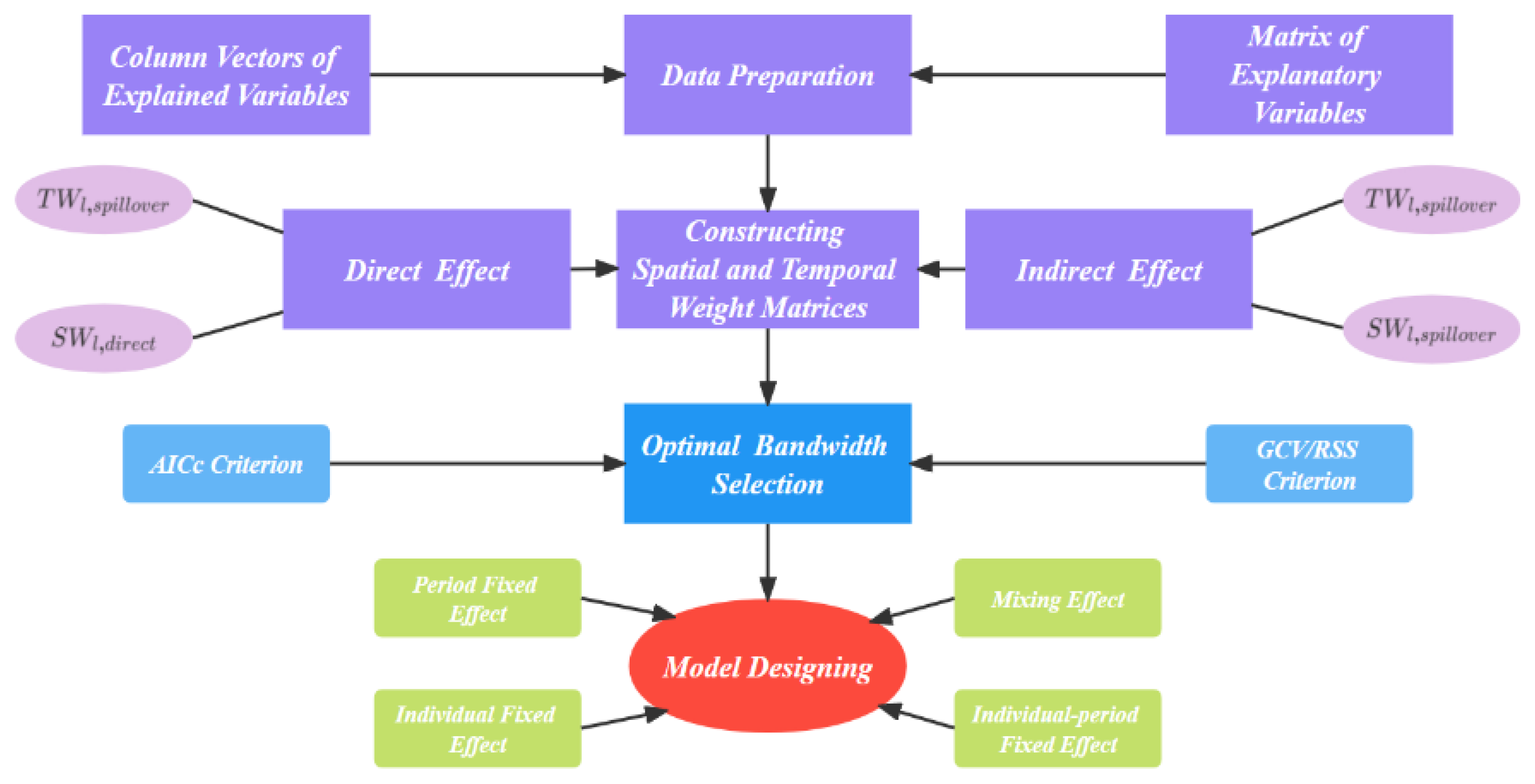
2.1. PGTWR Model
2.2. Construction of the Empirical Model
2.3. Methods of Carbon Accounting
3. Results
3.1. PGTWR Estimation of Results
3.2. Temporal Heterogeneity Analysis of the Regression Coefficient of Influencing Factors of Carbon Emission
3.2.1. Temporal Heterogeneity Analysis of the Influence of Industrial Structure on Carbon Emission
3.2.2. Temporal Heterogeneity Analysis of the Impact of Urbanization Level on Carbon Emission
3.2.3. Temporal Heterogeneity Analysis of the Impact of Energy Intensity on Carbon Emission
3.2.4. Temporal Heterogeneity Analysis of the Impact of Level of Economic Development on Carbon Emission
3.2.5. Temporal Heterogeneity Analysis of the Impact of Population Size on Carbon Emission
3.2.6. Temporal Heterogeneity Analysis of the Impact of Opening-Up on Carbon Emission
3.3. Spatial Heterogeneity Analysis of Regression Coefficient of Influencing Factors of Carbon Emission
4. Conclusions and Policy Recommendations
4.1. Conclusions
4.2. Policy Recommendations
Author Contributions
Funding
Institutional Review Board Statement
Informed Consent Statement
Data Availability Statement
Acknowledgments
Conflicts of Interest
References
- Xie, Z.H.; Liu, B.; Yan, X.D.; Meng, C.L.; Xu, X.L.; Liu, Y.; Qing, P.H.; Jia, B.H.; Xie, J.B.; Li, R.C.; et al. Assessment of Urban Planning Implementation effect in Response to Climate Change. Prog. Geogr. 2020, 1, 120–131. [Google Scholar] [CrossRef]
- Wang, Y.; Chen, W.; Kang, Y.; Li, W.; Guo, F. Spatial correlation of factors affecting CO2 emission at provincial level in China: A geographically weighted regression approach. J. Clean. Prod. 2018, 184, 929–937. [Google Scholar] [CrossRef]
- Dong, F.; Li, J.; Wang, Y.; Zhang, X.; Zhang, S. Drivers of the decoupling indicator between the economic growth and energy-related CO2 in China: A revisit from the perspectives of decomposition and spatiotemporal heterogeneity. Sci. Total Environ. 2019, 692, 631–658. [Google Scholar] [CrossRef] [PubMed]
- Liu, F.Y.; Liu, C.Z. Regional disparity, spatial spillover effects of urbanisation and carbon emissions in China. J. Clean. Prod. 2019, 241, 118226. [Google Scholar] [CrossRef]
- Zhang, W.S.; Cui, Y.Z.; Wang, J.H.; Wang, C.; Streets, D.G. How does urbanization affect co2 emissions of central heating systems in China? An assessment of natural gas transition policy based on nighttime light data—ScienceDirect. J. Clean. Prod. 2020, 276, 123188. [Google Scholar] [CrossRef]
- Wang, C.; Chen, J.N.; Zou, J. Decomposition of energy-related CO2 emission in China: 1957–2000. Energy 2005, 30, 73–83. [Google Scholar] [CrossRef]
- Liu, L.C.; Fan, Y.; Wu, G.; Wei, Y.M. Using LMDI method to analyze the change of China’s industrial CO2 emissions from final fuel use: An empirical analysis. Energy Policy 2007, 35, 5892–5900. [Google Scholar] [CrossRef]
- Freitas, L.; Kaneko, S. Decomposing the decoupling of CO2 emissions and economic growth in Brazil. Ecol. Econ. 2011, 70, 1459–1469. [Google Scholar] [CrossRef]
- Fan, Y.; Liu, L.C.; Wu, G.; Wei, Y.M. Analyzing impact factors of CO2 emissions using the STIRPAT model. Environ. Impact Assess. Rev. 2006, 26, 377–395. [Google Scholar] [CrossRef]
- Shahbaz, M.; Loganathan, N.; Muzaffar, A.T.; Ahmed, K.; Jabran, M.A. How urbanization affects CO2 emissions in Malaysia? The application of STIRPAT model. Renew. Sustain. Energy Rev. 2016, 57, 83–93. [Google Scholar] [CrossRef] [Green Version]
- Li, L.; Hong, X.F. Spatial Effects of Energy-Related Carbon Emissions and Environmental Pollution—STIRPAT Durbin Model Based on Energy Intensity and Technology Progress. J. Ind. Technol. Econ. 2017, 9, 65–72. [Google Scholar]
- Li, K.; Fang, L.T. Profile Estimation of Spatial Lag Quantile Regression Model. J. Quant. Tech. Econ. 2018, 10, 144–161. [Google Scholar]
- Brunsdon, C.; Fotheringham, A.S.; Charlton, M. Geographically weighted regression: A method for exploring spatial non-stationarity. Geogr. Anal. 1996, 28, 281–298. [Google Scholar] [CrossRef]
- Pavlov, A.D. Space varying regression coefficients: A semi-parametric approach applied to real estate markets. Real Estate Econ. 2003, 28, 249–283. [Google Scholar] [CrossRef]
- Fotheringham, L. Geographically weighted regression using a non-Euclidean distance metric with a study on London house price data. Procedia Environ. Sci. 2011, 7, 92–97. [Google Scholar] [CrossRef] [Green Version]
- Geng, J.; Kai, C.; Le, Y.; Yong, T. Geographically weighted regression model (GWR) based spatial analysis of house price in Shenzhen. In Proceedings of the 19th International Conference on Geoinformatics, Shanghai, China, 24–26 June 2011. [Google Scholar] [CrossRef]
- Li, F.X.; Li, M.C.; Liang, J. Study on disparity of regional economic development based on geoinformatic TUPU and GWR model: A case of growth of GDP per capita in China from 1999 to 2003. Int. Soc. Opt. Photonics 2007, 6754, 67543A. [Google Scholar] [CrossRef]
- Chu, E.M.; Xu, X.P. Studies on the Relationship between Export and Regional Economic Growth under the Endogenous Growth Framework: An Empirical Analysis Based on GWR Model. Available online: http://en.cnki.com.cn/Article_en/CJFDTotal-TJLT201112007.htm (accessed on 5 March 2022).
- Qian, Q.; Fan, Q.; Zhou, P.F. An integrated analysis of GWR models and spatial econometric global models to decompose the driving forces of the township consumption development in Gansu, China. Sustainability 2021, 14, 281. [Google Scholar] [CrossRef]
- Nematoollah, A.; Shekufeh, F.; Somayeh, J. Spatial analysis of the effect of government’s fiscal policy on income distribution inequality in Iran: (GWR1 approach). J. Quant. Econ. 2021, 8, 1–25. [Google Scholar]
- Hao, W.U.; Li, M.Q. An analysis of spatial evolution of income distribution and influence factors in Guangdong province based on ESDA-GWR. Commer. Res. 2017, 59, 79. [Google Scholar]
- Bonnet, J.; Bourdin, S.; Gazzah, F. The entrepreneurial context and its spatially differentiated influence on the level of regional development. Rev. D’économie Régionale Urbaine 2019, 4, 699–725. [Google Scholar] [CrossRef]
- Wang, H.T.; Hu, X.H.; Ali, N. Spatial Characteristics and Driving Factors toward the Digital Economy: Evidence from Prefecture-Level Cities in China. J. Asian Financ. Econ. Bus. 2022, 9, 419–426. [Google Scholar] [CrossRef]
- Chen, Y.; Miao, Q.; Zhou, Q. Spatiotemporal Differentiation and Driving Force Analysis of the High-Quality Development of Urban Agglomerations along the Yellow River Basin. Int. J. Environ. Res. Public Health 2022, 19, 2484. [Google Scholar] [CrossRef] [PubMed]
- Lin, Y.Z.; Peng, C.; Shu, J.F.; Zhai, W.; Cheng, J.Q. Spatiotemporal characteristics and influencing factors of urban resilience efficiency in the Yangtze River Economic Belt, China. Environ. Sci. Pollut. Res. 2022, 29, 39807–39826. [Google Scholar] [CrossRef] [PubMed]
- Quan, W.; Jian, N.; Tenhunen, J. Application of a geographically-weighted regression analysis to estimate net primary production of Chinese forest ecosystems. Glob. Ecol. Biogeogr. 2010, 14, 379–393. [Google Scholar] [CrossRef]
- Fan, X.; Gu, X.; Yu, H.; Long, A.; Tiando, D.S.; Ou, S.; Li, J.; Rong, Y.; Tang, G.; Zheng, Y.; et al. The Spatial and Temporal Evolution and Drivers of Habitat Quality in the Hung River Valley. Land 2021, 10, 1369. [Google Scholar] [CrossRef]
- Wang, S.; Fang, C.; Ma, H.; Wang, Y.; Qin, J. Spatial differences and multi-mechanism of carbon footprint based on GWR model in provincial China. J. Geogr. Sci. 2014, 24, 630. [Google Scholar] [CrossRef]
- Huang, B.; Wu, B.; Barry, M. Geographically and Temporally Weighted Regression for Modeling Spatiotemporal variation in house prices. Int. J. Geogr. Inf. Sci. 2010, 24, 383–401. [Google Scholar] [CrossRef]
- Liu, J.P.; Yang, Y.; Xu, S.H.; Zhao, Y.Y.; Wang, Y.; Zhang, F.H. A geographically temporal weighted regression approach with travel distance for house price estimation. Entropy 2016, 18, 303. [Google Scholar] [CrossRef]
- Xuan, H.Y.; Zhang, A.Q.; Lin, Q.L.; Chen, J.S. Affecting Factors Research of Chinese Provincial Economic Development—Based on GTWR Model. J. Ind. Technol. Econ. 2016, 2, 154–160. [Google Scholar]
- Zeng, Z.Z.; Qian, S.; Plaza, J.; Plaza, A.; Li, J. Spatial Downscaling for Global Precipitation Measurement Using a Geographically and Temporally Weighted Regression Model. In Proceedings of the IGARSS 2020–2020 IEEE International Geoscience and Remote Sensing Symposium, Waikoloa, HI, USA, 26 September–2 October 2020. [Google Scholar]
- Chu, H.J.; Kong, S.J.; Chang, C.H. Spatio-temporal water quality mapping from satellite images using geographically and temporally weighted regression. Int. J. Appl. Earth Obs. Geoinf. 2018, 65, 1–11. [Google Scholar] [CrossRef]
- Chu, H.J.; Huang, B.; Lin, C.Y. Modeling the spatio-temporal heterogeneity in the pm10-pm2.5 relationship. Atmos. Environ. 2015, 102, 176–182. [Google Scholar] [CrossRef]
- Chen, J.; Lian, X.; Su, H.; Zhang, Z.; Ma, X.; Chang, B. Analysis of China’s carbon emission driving factors based on the perspective of eight major economic regions. Environ. Sci. Pollut. Res. 2021, 28, 8181–8204. [Google Scholar] [CrossRef] [PubMed]
- Shi, T.; Zhang, W.; Zhou, Q.; Wang, K. Industrial structure, urban governance and haze pollution: Spatiotemporal evidence from China. Sci. Total Environ. 2020, 742, 139228. [Google Scholar] [CrossRef] [PubMed]
- Wang, H.J.; Zhang, B.; Liu, Y.L.; Xu, S.; Zhao, Y.T.; Chen, Y.; Hong, S. Urban expansion patterns and their driving forces based on the center of gravity-GTWR model: A case study of the Beijing-Tianjin-Hebei urban agglomeration. J. Geogr. Sci. 2020, 30, 297–318. [Google Scholar] [CrossRef]
- Fan, Q.; Guo, A.J. A New Geographically and Temporally Weighted Regression Model for Panel Data Based on Holographic Mapping. J. Quant. Tech. Econ. 2021, 4, 120–138. [Google Scholar]
- Dietz, T.; Rosa, E.A. Rethinking the environmental impacts of population, affluence and technology. Hum. Ecol. Rev. 1994, 2, 277–300. [Google Scholar]
- York, R.; Rosa, E.A.; Dietz, T. STIRPAT, IPAT and ImPACT: Analytic tools for unpacking the driving forces of environmental impacts. Ecol. Econ. 2003, 46, 351–365. [Google Scholar] [CrossRef]
- Fang, K.; Tang, Y.; Zhang, Q.; Song, J.; Wen, Q.; Sun, H.; Ji, C.; Xu, A. Will China peak its energy-related carbon emissions by 230? Lessons from 30 Chinese provinces. Appl. Energy 2019, 255, 113852. [Google Scholar] [CrossRef]
- Xu, S.C.; He, Z.X.; Long, R.Y. Factors that influence carbon emissions due to energy consumption in China: Decomposition analysis using LMDI. Appl. Energy 2014, 127, 182–193. [Google Scholar] [CrossRef]
- Intergovernmental Panel on Climate Change (IPCC). IPCC Guidelines for National Greenhouse Gas Inventories. 2006. Available online: http://www.ipcc-nggip.iges.or.jp/public/2006gl/index.html (accessed on 6 March 2022).
- Yu, S.W.; Wei, Y.M.; Guo, H.X.; Ding, L.P. Carbon emission coefficient measurement of the coal-to-power energy chain in China—ScienceDirect. Appl. Energy 2014, 114, 290–300. [Google Scholar] [CrossRef]
- Zhang, L.L.; Long, R.; Hong, C. Carbon emission reduction potential of urban rail transit in China based on electricity consumption structure. Resour. Conserv. Recycl. 2019, 142, 113–121. [Google Scholar] [CrossRef]
- Li, Z.; Li, G. Characteristics and Causes of Chinese Urban Energy. Ind. Econ. Res. 2010, 02, 25–30. [Google Scholar]
- Yang, Z.H. Factors Price Distortion, FDI and Urban Energy Efficiency—Empirical Study Based on the Prefecture-Level Cities. J. Financ. Econ. 2016, 12, 26–31. [Google Scholar]
- Cole, M.A.; Neumayer, E. Examining the impact of demographic factors on air pollution. Popul. Environ. 2004, 26, 5–21. [Google Scholar] [CrossRef] [Green Version]
- Li, J.; Wang, Y.; Wang, Y. Decoupling Analysis and Influence Factors between Resource Environment and Economic Growth in Beijing-Tianjin-Hebei Region. Econ. Geogr. 2019, 39, 43–49. [Google Scholar]


| Variable | Variable Meaning | Unit | Data Source |
|---|---|---|---|
| Carbon emissions | CO2 emissions from fossil fuels | 10,000 ton | See Section 2.3 |
| Industrial structure | Proportion of output value of secondary industry | % | Local Statistical Yearbook |
| Urbanization level | Land area of urban construction | Square kilometers | China City Statistical Yearbook |
| Energy intensity | Energy consumption per unit of GDP | Tons of standard/100 million yuan | Local Statistical Yearbook |
| Level of economic development | GDP | One hundred million yuan | Chinese Statistical yearbook |
| Population size | Population of permanent residents | Ten thousand people | Local Statistical Yearbook |
| Opening up | Amount of foreign investment actually utilized | Thousands of dollars | Local Statistical Yearbook |
| Energy | Average Low Emission | Standard Coal Coefficient | Carbon Content Per Calorific Value | Carbon Oxidation Rate | CO2 Emission Coefficient |
|---|---|---|---|---|---|
| Coke | 28,435 KJ/kg | 0.7143 kgce/kg | 26.37 tons of carbon/TJ | 0.93% | 1.9003 kg-CO2/kg |
| Natural gas of oil field | 38.931 kg/m3 | 1.3300 kgce/m3 | 15.3 tons of carbon/TJ | 0.99% | 2.1622 kg-CO2/m3 |
| Raw coal | 20,908 KJ/kg | 0.7143 kgce/kg | 26.37 tons of carbon/TJ | 0.94% | 1.9003 kg-CO2/kg |
| Crude oil | 41,816 KJ/kg | 1.4286 kgce/kg | 20.1 tons of carbon/TJ | 0.98% | 3.0202 kg-CO2/kg |
| Fuel oil | 41,816 KJ/kg | 1.4286 kgce/kg | 21.1 tons of carbon/TJ | 0.98% | 3.1705 kg-CO2/kg |
| petroleum | 43,070 KJ/kg | 1.4714 kgce/kg | 18.9 tons of carbon /TJ | 0.98% | 2.9251 kg-CO2/kg |
| kerosene | 43,070 KJ/kg | 1.4714 kgce/kg | 19.5 tons of carbon/TJ | 0.98% | 3.0179 kg-CO2/kg |
| diesel | 42,652 KJ/kg | 1.4571 kgce/kg | 20.2 tons of carbon/TJ | 0.98% | 3.0959 kg-CO2/kg |
| Liquefied petroleum gas | 50,179 KJ/kg | 1.7143 kgce/kg | 17.2 tons of carbon/TJ | 0.98% | 3.1013 kg-CO2/kg |
| AICc Criterion (Optimal Spatial Bandwidth = 13, Optimal Temporal Bandwidth = 6) | GCV\RSS Criterion (Optimal Spatial Bandwidth = 7, Optimal Temporal Bandwidth = 6) | |||||||
|---|---|---|---|---|---|---|---|---|
| Mixing Effect | Individual Fixed Effect | Period Fixed Effect | Individual–Period Fixed Effect | Mixing Effect | Individual Fixed Effect | Period Fixed Effect | Individual–Period Fixed Effect | |
| significance ratio of the estimate of local coefficient | 0.8919 | 0.3397 | 0.9679 | 0.4423 | 0.6703 | 0.2885 | 0.6688 | 0.3376 |
| Sample size | 78 | 78 | 78 | 78 | 78 | 78 | 78 | 78 |
| Degree of freedom | 31 | 32 | 31 | 32 | 15 | 15 | 15 | 15 |
| Estimate of Variance of stochastic disturbance | 13.835 | 0.538 | 1.928 | 16.832 | 28.157 | 1.087 | 2.956 | 32.830 |
| Value of CV criterion | 428.9 | 17.2 | 59.8 | 538.6 | 422.4 | 16.3 | 44.3 | 492.4 |
| Value of GCV criterion | 0.0851 | 0.0034 | 0.0119 | 0.1069 | 0.0838 | 0.0032 | 0.0088 | 0.0977 |
| Value of AICc criterion | 448.1 | 192.2 | 291.7 | 461.2 | 501.7 | 245.2 | 323.5 | 511.3 |
| Modified goodness of fit | 0.9996 | 0.9814 | 0.9952 | 0.9999 | 0.9998 | 0.9319 | 0.9880 | 0.9999 |
| F statistical value | 48,378 | 1035 | 4521 | 3,822,745 | 80,040 | 264 | 1581 | 244,461 |
| F probability of statistics | 0.000 | 0.000 | 0.000 | 0.000 | 0.000 | 0.000 | 0.000 | 0.000 |
| Modified critical value of probability (α = 0.01, 0.05, 0.1) | 0.0169 0.0844 0.1688 | 0.0171 0.0853 0.1706 | 0.0202 0.1012 0.2024 | 0.0185 0.0924 0.1849 | 0.0149 0.0745 0.1489 | 0.0159 0.0796 0.1592 | 0.0178 0.0888 0.1775 | 0.0166 0.0829 0.1658 |
| logarithmic likelihood values | −213.1 | −86.5 | −136.3 | −220.8 | −240.9 | −113.9 | −152.9 | −246.8 |
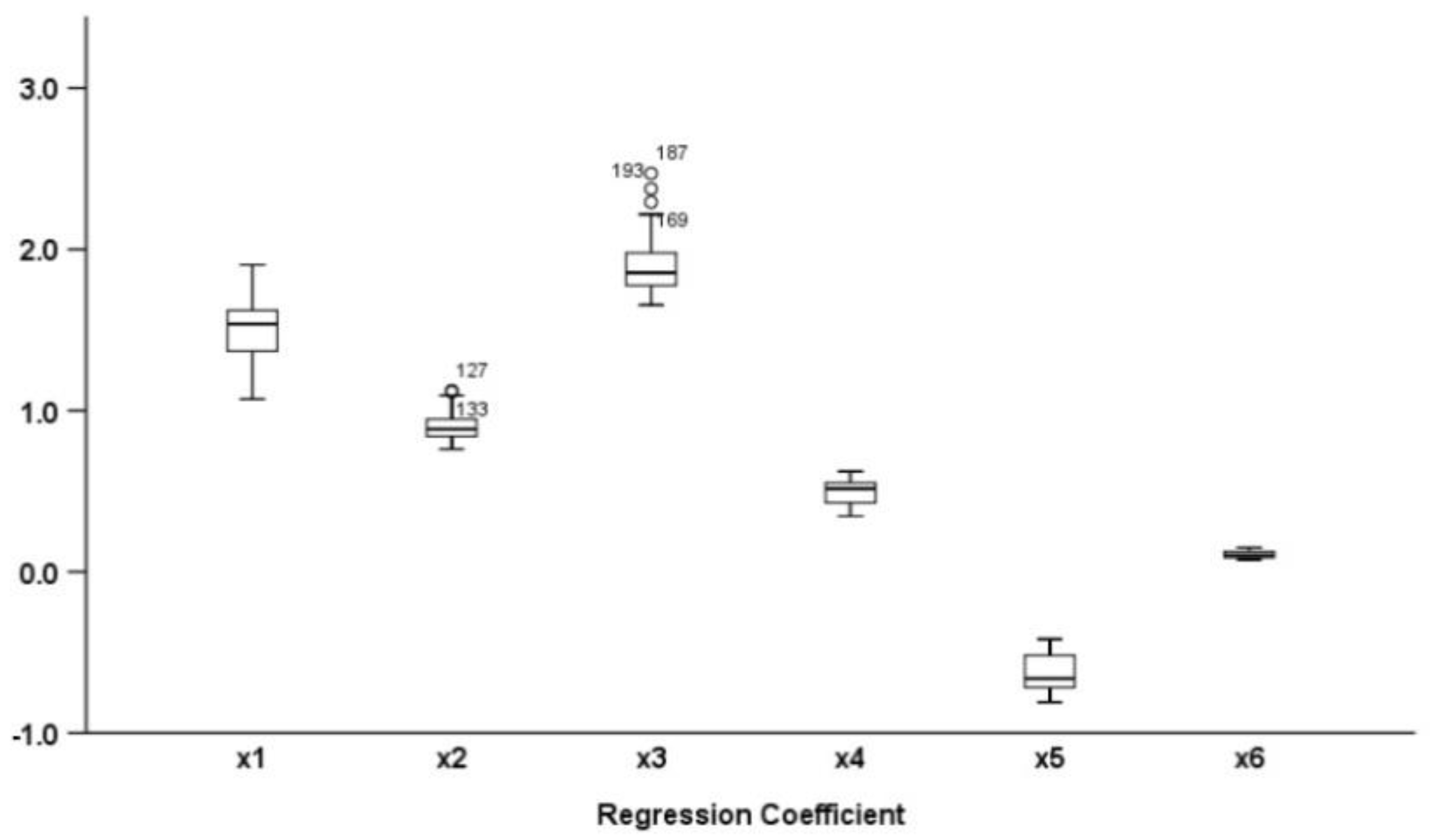
| Variable | Minimum | Maximum | Average | Upper Quartile | Lower Quartile | Quartile Range | Standard Deviation |
|---|---|---|---|---|---|---|---|
| X1 | 1.07 | 1.90 | 1.51 | 1.38 | 1.62 | 0.23 | 0.18 |
| X2 | 0.76 | 1.12 | 0.90 | 0.84 | 0.94 | 0.10 | 0.09 |
| X3 | 1.65 | 2.47 | 1.90 | 1.78 | 1.98 | 0.19 | 0.16 |
| X4 | 0.35 | 0.62 | 0.50 | 0.43 | 0.55 | 0.12 | 0.07 |
| X5 | −0.81 | −0.42 | −0.63 | −0.71 | −0.52 | 0.19 | 0.11 |
| X6 | 0.08 | 0.15 | 0.11 | 0.09 | 0.13 | 0.04 | 0.02 |
Publisher’s Note: MDPI stays neutral with regard to jurisdictional claims in published maps and institutional affiliations. |
© 2022 by the authors. Licensee MDPI, Basel, Switzerland. This article is an open access article distributed under the terms and conditions of the Creative Commons Attribution (CC BY) license (https://creativecommons.org/licenses/by/4.0/).
Share and Cite
Lou, T.; Ma, J.; Liu, Y.; Yu, L.; Guo, Z.; He, Y. A Heterogeneity Study of Carbon Emissions Driving Factors in Beijing-Tianjin-Hebei Region, China, Based on PGTWR Model. Int. J. Environ. Res. Public Health 2022, 19, 6644. https://doi.org/10.3390/ijerph19116644
Lou T, Ma J, Liu Y, Yu L, Guo Z, He Y. A Heterogeneity Study of Carbon Emissions Driving Factors in Beijing-Tianjin-Hebei Region, China, Based on PGTWR Model. International Journal of Environmental Research and Public Health. 2022; 19(11):6644. https://doi.org/10.3390/ijerph19116644
Chicago/Turabian StyleLou, Ting, Jianhui Ma, Yu Liu, Lei Yu, Zhaopeng Guo, and Yan He. 2022. "A Heterogeneity Study of Carbon Emissions Driving Factors in Beijing-Tianjin-Hebei Region, China, Based on PGTWR Model" International Journal of Environmental Research and Public Health 19, no. 11: 6644. https://doi.org/10.3390/ijerph19116644
APA StyleLou, T., Ma, J., Liu, Y., Yu, L., Guo, Z., & He, Y. (2022). A Heterogeneity Study of Carbon Emissions Driving Factors in Beijing-Tianjin-Hebei Region, China, Based on PGTWR Model. International Journal of Environmental Research and Public Health, 19(11), 6644. https://doi.org/10.3390/ijerph19116644