
The Relationship between Urban Population Density Distribution and Land Use in Guangzhou, China: A Spatial Spillover Perspective

Abstract
:1. Introduction
2. Literature Review
2.1. Urban Population Density Distribution
2.2. Population Density Distribution and Land Use
3. Methodology
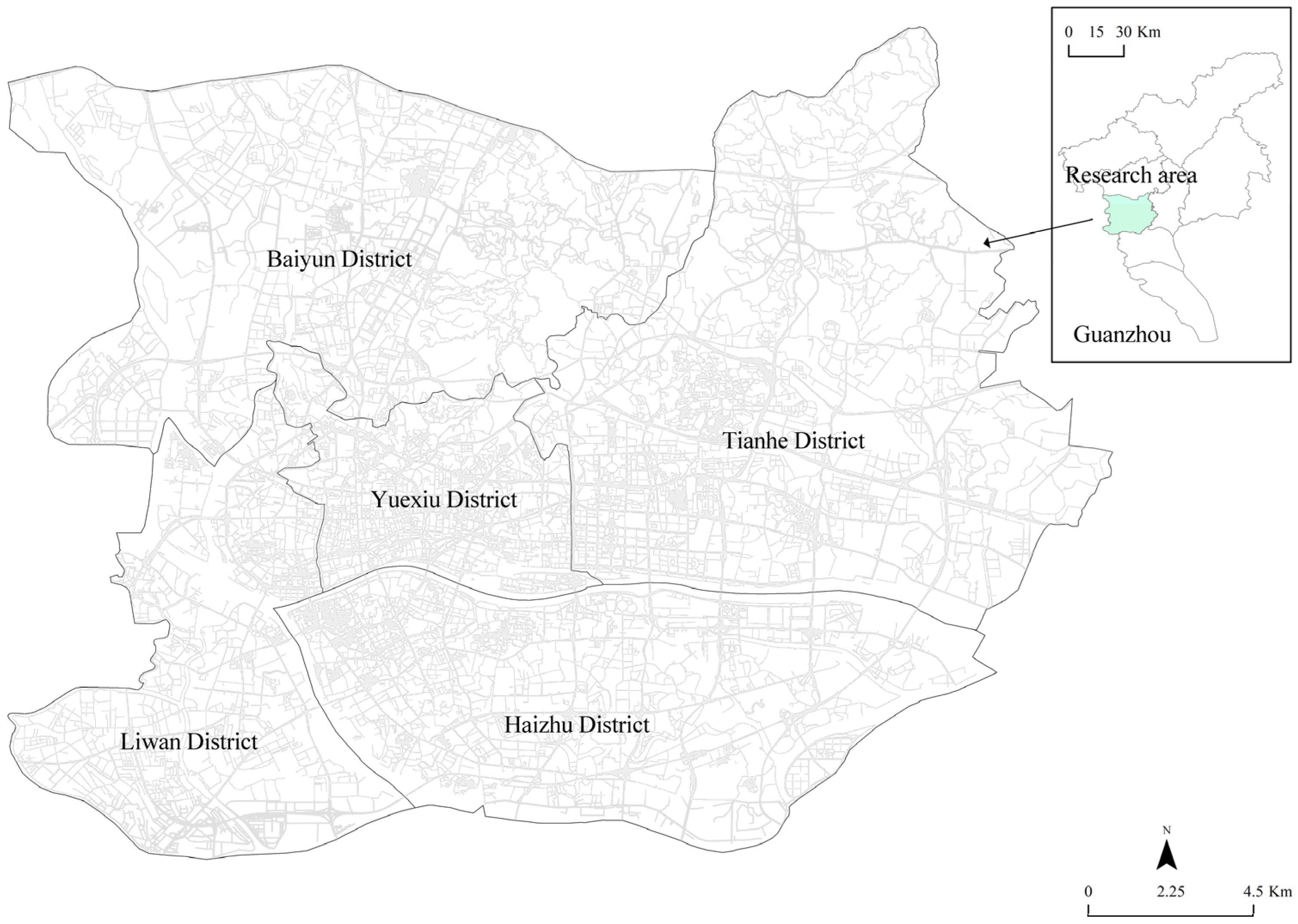
3.1. Research Area
3.2. Data Collection
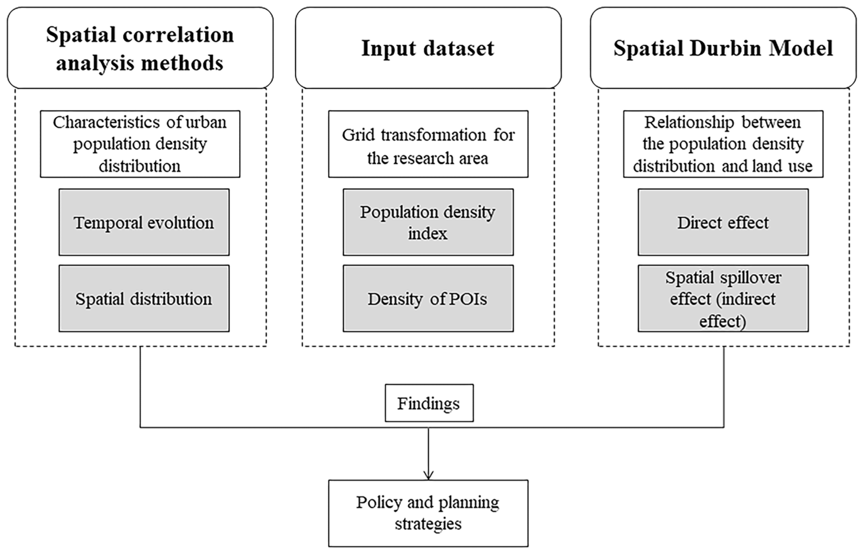
3.3. Analysis Framework
3.3.1. Population Density Index (PDI)
3.3.2. Spatial Correlation Analysis Methods
3.3.3. Spatial Durbin Model (SDM)
4. Results
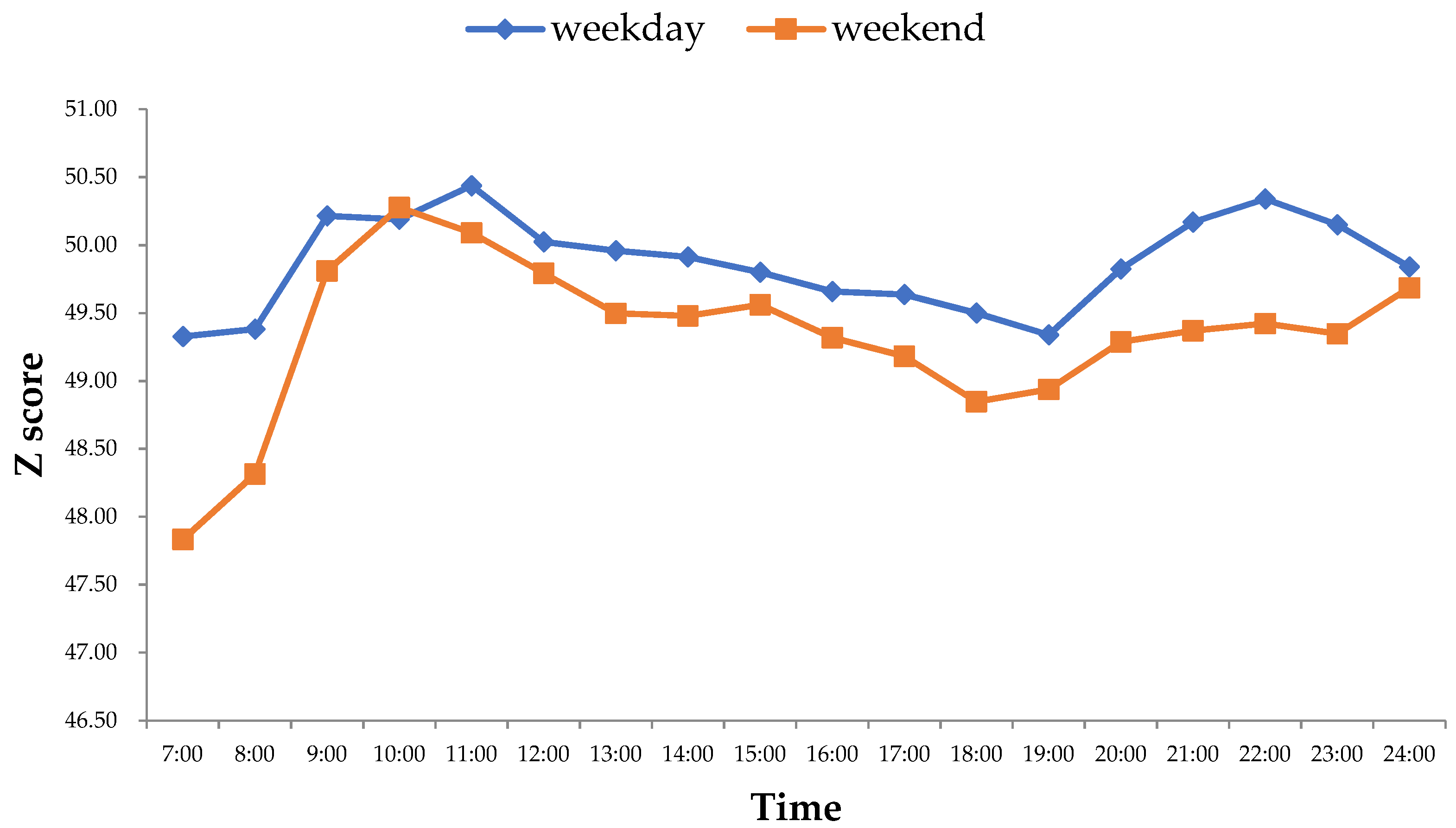
4.1. The Temporal Evolution Characteristics of Urban Population Density
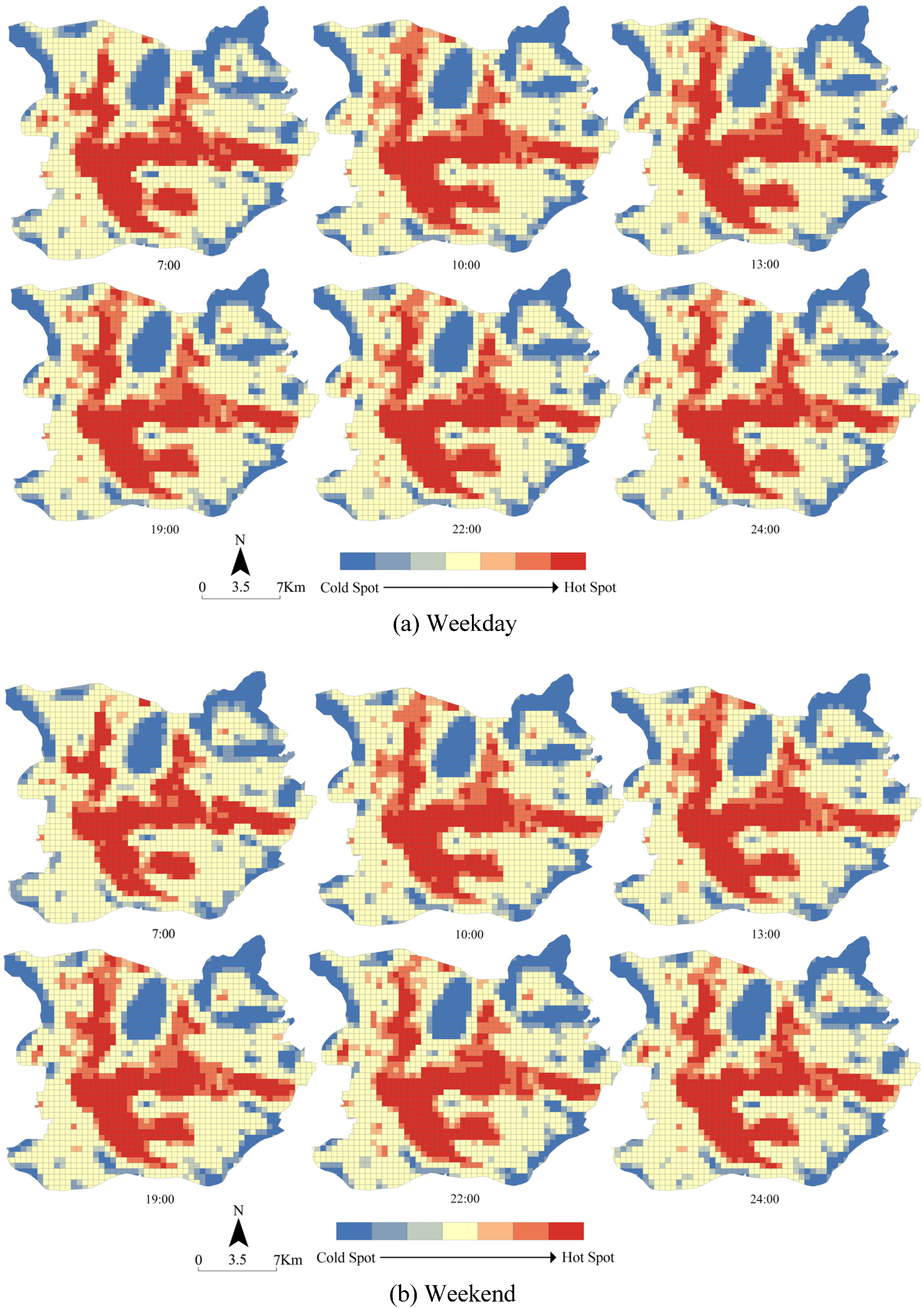
4.2. The Spatial Distribution Characteristics of Urban Population Density
4.3. The Relationship between Urban Population Density and Land Use
5. Discussion
5.1. Characteristics of Urban Population Density Distribution
5.2. The Impact Mechanism of Urban Population Density Distribution
6. Conclusions
Author Contributions
Funding
Institutional Review Board Statement
Informed Consent Statement
Data Availability Statement
Conflicts of Interest
References
- Jia, P.; Qiu, Y.L.; Gaughan, A.E. A fine-scale spatial population distribution on the High-resolution Gridded Population Surface and application in Alachua County, Florida. Appl. Geogr. 2014, 50, 99–107. [Google Scholar] [CrossRef]
- Murray, A.T.; Davis, R.; Stimson, R.J.; Ferreira, L. Public transportation access. Transport. Res. Part D Transport. Environ. 1998, 3, 319–328. [Google Scholar] [CrossRef] [Green Version]
- Gao, Z.Q.; Tan, N.R.; Geddes, R.R.; Ma, T. Population Distribution Characteristics and Spatial Planning Response Analysis in Metropolises: A Case Study of Beijing. Int. Rev. Spat. Plan. Sustain. Dev. 2019, 7, 134–154. [Google Scholar] [CrossRef]
- Goodman, A.; Sahlqvist, S.; Ogilvie, D.; Connect, C. New Walking and Cycling Routes and Increased Physical Activity: One- and 2-Year Findings from the UK iConnect Study. Am. J. Public Health 2014, 104, E38–E46. [Google Scholar] [CrossRef] [PubMed]
- Eom, S.; Suzuki, T. Spatial distribution of pedestrian space in central Tokyo Regarding building, public transportation and urban renewal projects. Int. Rev. Spat. Plan. Sustain. Dev. 2019, 7, 108–124. [Google Scholar] [CrossRef] [Green Version]
- Deng, C.; Wu, C.; Wang, L. Improving the housing-unit method for small-area population estimation using remote-sensing and GIS information. Int. J. Remote. Sens. 2010, 31, 5673–5688. [Google Scholar] [CrossRef]
- Li, M.Y.; Shen, Z.J.; Hao, X.H. Revealing the relationship between spatio-temporal distribution of population and urban function with social media data. GeoJournal 2016, 81, 919–935. [Google Scholar] [CrossRef]
- Zhang, X.C.; Sun, Y.R.; Chan, T.O.; Huang, Y.; Zheng, A.Y.; Liu, Z. Exploring Impact of Surrounding Service Facilities on Urban Vibrancy Using Tencent Location-Aware Data: A Case of Guangzhou. Sustainability 2021, 13, 444. [Google Scholar] [CrossRef]
- Shi, Y.; Yang, J.; Shen, P. Revealing the correlation between population density and the spatial distribution of urban public service facilities with mobile phone data. ISPRS Int. J. Geo Inf. 2020, 9, 38. [Google Scholar] [CrossRef] [Green Version]
- Qian, J.H.; Yang, C.H.; Han, D.D.; Ma, Y.G. Multi-scaling mix and non-universality between population and facility density. Phys. A Stat. Mech. Its Appl. 2012, 391, 5146–5152. [Google Scholar] [CrossRef] [Green Version]
- Li, J.G.; Li, J.W.; Yuan, Y.Z.; Li, G.F. Spatiotemporal distribution characteristics and mechanism analysis of urban population density: A case of Xi’an, Shaanxi, China. Cities 2019, 86, 62–70. [Google Scholar] [CrossRef]
- Feng, D.Y.; Tu, L.L.; Sun, Z.W. Research on Population Spatiotemporal Aggregation Characteristics of a Small City: A Case Study on Shehong County Based on Baidu Heat Maps. Sustainability 2019, 11, 6276. [Google Scholar] [CrossRef] [Green Version]
- Shi, P.P.; Xiao, Y.H.; Zhan, Q.M. A Study on Spatial and Temporal Aggregation Patterns of Urban Population in Wuhan City based on Baidu Heat Map and POI Data. Int. Rev. Spat. Plan. Sustain. Dev. 2020, 8, 101–121. [Google Scholar] [CrossRef]
- Liu, X.Q.; Huang, B.; Li, R.R.; Wang, J.H. Characterizing the complex influence of the urban built environment on the dynamic population distribution of Shenzhen, China, using geographically and temporally weighted regression. Env. Plan. B Urban Anal. City Sci. 2021, 48, 1445–1462. [Google Scholar] [CrossRef]
- Wu, C.; Ye, X.Y.; Ren, F.; Du, Q.Y. Check-in behaviour and spatio-temporal vibrancy: An exploratory analysis in Shenzhen, China. Cities 2018, 77, 104–116. [Google Scholar] [CrossRef]
- Shi, Z.; Zhou, S.; Chen, Y. Jobs-housing relationship in different industries and its impact on traffic demand on road networks: A case study in Guangzhou. City Plan. Rev. 2020, 44, 87–94. [Google Scholar] [CrossRef]
- Barreca, A.; Curto, R.; Rolando, D. Urban Vibrancy: An Emerging Factor that Spatially Influences the Real Estate Market. Sustainability 2020, 12, 346. [Google Scholar] [CrossRef] [Green Version]
- Bagan, H.; Yamagata, Y. Analysis of urban growth and estimating population density using satellite images of nighttime lights and land-use and population data. GISci. Remote Sens. 2015, 52, 765–780. [Google Scholar] [CrossRef]
- Ni, L.; Wang, X.C.; Chen, X.M. A spatial econometric model for travel flow analysis and real-world applications with massive mobile phone data. Transp. Res. Part C Emerg. Technol. 2018, 86, 510–526. [Google Scholar] [CrossRef]
- Sun, X. Spatialization and Autocorrelation Analysis of Urban Population Kernel Density Supported by Nighttime Light Remote Sensing. J. Geo Inf. Sci. 2020, 22, 2256–2266. [Google Scholar] [CrossRef]
- Zeng, C.; Song, Y.; Cai, D.W.; Hu, P.Y.; Cui, H.T.; Yang, J.; Zhang, H.X. Exploration on the spatial spillover effect of infrastructure network on urbanization: A case study in Wuhan urban agglomeration. Sust. Cities Soc. 2019, 47, 101476. [Google Scholar] [CrossRef]
- Kang, C.; Liu, Y.; Ma, X.; Wu, L. Towards Estimating Urban Population Distributions from Mobile Call Data. J. Urban Technol. 2012, 19, 3–21. [Google Scholar] [CrossRef]
- Shaw, S.L.; Tsou, M.H.; Ye, X.Y. Editorial: Human dynamics in the mobile and big data era. Int. J. Geogr. Inf. Sci. 2016, 30, 1687–1693. [Google Scholar] [CrossRef]
- Song, C.M.; Qu, Z.H.; Blumm, N.; Barabasi, A.L. Limits of Predictability in Human Mobility. Science 2010, 327, 1018–1021. [Google Scholar] [CrossRef] [PubMed] [Green Version]
- Zhao, P.J.; Lu, B.; de Roo, G. Impact of the jobs-housing balance on urban commuting in Beijing in the transformation era. J. Transp. Geogr. 2011, 19, 59–69. [Google Scholar] [CrossRef]
- Lung, T.; Lubker, T.; Ngochoch, J.K.; Schaab, G. Human population distribution modelling at regional level using very high resolution satellite imagery. Appl. Geogr. 2013, 41, 36–45. [Google Scholar] [CrossRef]
- Cai, J.X.; Huang, B.; Song, Y.M. Using multi-source geospatial big data to identify the structure of polycentric cities. Remote Sens. Environ. 2017, 202, 210–221. [Google Scholar] [CrossRef]
- Wu, Z.; Ye, Z. Research on urban spatial structure based on Baidu heat map: A study on the central city of Shanghai. City Plan. Rev. 2016, 40, 33–40. [Google Scholar] [CrossRef]
- Lyu, F.N.; Zhang, L. Using multi-source big data to understand the factors affecting urban park use in Wuhan. Urban For. Urban Green. 2019, 43, 126367. [Google Scholar] [CrossRef]
- Zeng, P.; Sun, Z.; Chen, Y.; Qiao, Z.; Cai, L. COVID-19: A Comparative Study of Population Aggregation Patterns in the Central Urban Area of Tianjin, China. Int. J. Environ. Res. Public Health 2021, 18, 2135. [Google Scholar] [CrossRef]
- Wang, L. Spatial-temporal Characteristics of Urban Population Aggregation Based on Baidu Heat Map in Central Areas of Wuhan City. J. Hum. Settl. West China 2018, 33, 52–56. [Google Scholar] [CrossRef]
- Zhang, Y.; Li, Q. The spatial characteristics of catering industry and its coupling analysis with dynamic population in the main city of Wuhan. J. Cent. China Norm. Univ. Nat. Sci. Ed. 2019, 53, 121–129. [Google Scholar] [CrossRef] [Green Version]
- Garcia-Palomares, J.C.; Salas-Olmedo, M.H.; Moya-Gomez, B.; Condeco-Melhorado, A.; Gutierrez, J. City dynamics through Twitter: Relationships between land use and spatiotemporal demographics. Cities 2018, 72, 310–319. [Google Scholar] [CrossRef]
- Ahas, R.; Aasa, A.; Silm, S.; Tiru, M. Daily rhythms of suburban commuters’ movements in the Tallinn metropolitan area: Case study with mobile positioning data. Transp. Res. Pt. C Emerg. Technol. 2010, 18, 45–54. [Google Scholar] [CrossRef]
- Tu, W.; Zhu, T.; Xia, J.; Zhou, Y.; Lai, Y.; Jiang, J.; Li, Q. Portraying the spatial dynamics of urban vibrancy using multisource urban big data. Comput. Environ. Urban Syst. 2020, 80, 101428. [Google Scholar] [CrossRef]
- Chen, W.; Liu, L.; Liang, Y. Retail center recognition and spatial aggregating feature analysis of retail formats in Guangzhou based on POI data. Geogr. Res. 2016, 35, 703–716. [Google Scholar] [CrossRef]
- Hao, F.; Wang, S.; Feng, Z.; Yu, T.; Ma, L. Spatial pattern and its industrial distribution of commercial space in Changchun based on POI data. Geogr. Res. 2018, 37, 366–378. [Google Scholar] [CrossRef]
- Sun, B.D.; Ermagun, A.; Dan, B. Built environmental impacts on commuting mode choice and distance: Evidence from Shanghai. Transport. Res. Part D Transport. Environ. 2017, 52, 441–453. [Google Scholar] [CrossRef]
- Ma, X.L.; Zhang, J.Y.; Ding, C.; Wang, Y.P. A geographically and temporally weighted regression model to explore the spatiotemporal influence of built environment on transit ridership. Comput. Environ. Urban Syst. 2018, 70, 113–124. [Google Scholar] [CrossRef]
- Huang, Y.H.; Zhao, C.P.; Song, X.Y.; Chen, J.; Li, Z.H. A semi-parametric geographically weighted (S-GWR) approach for modeling spatial distribution of population. Ecol. Indic. 2018, 85, 1022–1029. [Google Scholar] [CrossRef]
- Tobler, W.R. A computer movie simulating urban growth in the Detroit region. Econ. Geogr. 1970, 46, 234–240. [Google Scholar] [CrossRef]
- Tong, Q.; Qiu, F. Population growth and land development: Investigating the bi-directional interactions. Ecol. Econ. 2020, 169, 106505. [Google Scholar] [CrossRef]
- Jun, H.-J. Spillover effects in neighborhood housing value change: A spatial analysis. Hous. Stud. 2020. [Google Scholar] [CrossRef]
- da Silva, D.F.C.; Elhorst, J.P.; Neto, R.D.S. Urban and rural population growth in a spatial panel of municipalities. Reg. Stud. 2017, 51, 894–908. [Google Scholar] [CrossRef] [Green Version]
- LeSage, J.; Pace, R.K. Introduction to Spatial Econometrics; CRC Press/Taloy & Francis: Boca Raton, FL, USA, 2009. [Google Scholar]
- Elhorst, J.P. Applied Spatial Econometrics: Raising the Bar. Spat. Econ. Anal. 2010, 5, 9–28. [Google Scholar] [CrossRef]
- Bingrong, L.; Ying, Y.; Daquan, H.; Zheng, Y. Big Data Based Job-residence Relation in Chongqing Metropolitan Area. Planner 2015, 31, 92–96. [Google Scholar]
- Getis, A.; Ord, J.K. The analysis of spatial association by use of distance statistics. Geogr. Anal. 1992, 24, 189–206. [Google Scholar] [CrossRef]
- Wang, S.; Chen, Y.; Huang, J.; Chen, N.; Lu, Y.; Mesbah, M. Macrolevel Traffic Crash Analysis: A Spatial Econometric Model Approach. Math. Probl. Eng. 2019, 2019, 1–10. [Google Scholar] [CrossRef] [Green Version]
- Sun, Y.; Sun, T.; Xi, Q. Influence factors and spillover effect of the innovation agglomeration in Beijing. Geogr. Res. 2017, 36, 2419–2431. [Google Scholar] [CrossRef]
- Meng, X.; Cao, J.N.; Wang, X.F.; Zhang, C.; Lv, J.S. Spatial characteristics of the human factors of soil erosion at the boundary of political divisions: A spatial approach. Catena 2021, 201, 105278. [Google Scholar] [CrossRef]
- Xu, X.; Wang, Y. Study on Spatial Spillover Effects of Logistics Industry Development for Economic Growth in the Yangtze River Delta City Cluster Based on Spatial Durbin Model. Multidiscip. Digit. Publ. Inst. 2017, 14, 1508. [Google Scholar] [CrossRef] [Green Version]
- Yang, L.; Zhou, L.; Zhang, X. Research and evaluation of Jobs-Housing Space Characteristics based on Mobile Phone Signaling Data: A Case Study of Guangzhou. Urban Insight. 2019, 87–96. [Google Scholar] [CrossRef]
- Li, Y.; Chen, T.; Li, X.; Xu, W.; Lang, W. Identification and Patterns of Employment and Residential Centers in a Cross-Border Region Based on Mobile Phone Signaling Data: A Case Study of Guangzhou and Foshan. Trop. Geogr. 2020, 40, 206–216. [Google Scholar] [CrossRef]
- Chen, T.; Hui, E.C.M.; Wu, J.; Lang, W.; Li, X. Identifying urban spatial structure and urban vibrancy in highly dense cities using georeferenced social media data. Habitat Int. 2019, 89, 102005. [Google Scholar] [CrossRef]
- Li, Y.; Chen, Q.; Zeng, R.; Chu, Q. Analysis of the distribution and usage characteristics of medical facilities based on big data. In Proceedings of the China Urban Planning Annual Conference, Hangzhou, China, 24 November 2018; p. 14. [Google Scholar]
- Lin, X.; Wang, G.; Hu, Y. Characteristics of the Jobs-Housing Balance in Central Guangzhou Based on Open Big Data. Trop. Geogr. 2020, 40, 254–265. [Google Scholar] [CrossRef]
- Yang, Z.; Chen, Y.; Qian, Q.; Hu, Y.; Huang, Q. Evaluation of the Matching Degree of Public Medical Service Level Based on Population Spatialization: A Case Study of Guangzhou. Geogr. Geo-Inf. Sci. 2019, 35, 74–82. [Google Scholar] [CrossRef]
- Wang, Y.; Yang, R.; Li, Q.; Xi, W. The Spatial Layout Features and Patterns of Banking Industry in Guangzhou City, China. Sci. Geogr. Sin. 2016, 36, 742–750. [Google Scholar] [CrossRef]
- Yuan, M.; Hanfa, X. Exploring the relationship between landscape characteristics and urban vibrancy: A case study using morphology and review data. Cities 2019, 95, 102389. [Google Scholar] [CrossRef]
- Lamb, R.F. The morphology and vitality of business districts in upstate New York villages. Prof. Geogr. 1985, 37, 162–172. [Google Scholar] [CrossRef]
- Li, Y.; Shi, T.; Zhang, Y.; Chen, W.; Wang, Z.; Li, H. Learning deep semantic segmentation network under multiple weakly-supervised constraints for cross-domain remote sensing image semantic segmentation. ISPRS J. Photogramm. Remote Sens. 2021, 175, 20–33. [Google Scholar] [CrossRef]
- Benjdira, B.; Bazi, Y.; Koubaa, A.; Ouni, K. Unsupervised domain adaptation using generative adversarial networks for semantic segmentation of aerial images. Remote Sens. 2019, 11, 1369. [Google Scholar] [CrossRef] [Green Version]

| Functions | POI Categories | Item Label | Mean | SD |
|---|---|---|---|---|
| Living | Density of housing POIs | HO | 0.0407 | 0.0794 |
| Density of life service POIs | LS | 0.0342 | 0.0693 | |
| Density of medical and health POIs | MH | 0.0322 | 0.0916 | |
| Working | Density of office POIs | OF | 0.0679 | 0.1321 |
| Density of finance and banking POIs | FB | 0.0536 | 0.1120 | |
| Density of government and social insurance POIs | GS | 0.0353 | 0.0677 | |
| Density of factory POIs | FA | 0.0196 | 0.0654 | |
| TransportationRecreation | Density of transportation POIs | TR | 0.0208 | 0.0351 |
| Density of food POIs | FO | 0.0276 | 0.0769 | |
| Density of entertainment POIs | EN | 0.0505 | 0.0772 | |
| Density of education and culture POIs | EC | 0.0263 | 0.0570 | |
| Density of tourism POIs | TO | 0.0217 | 0.0540 |
| Morning: 07:00 to 12:00 | Afternoon: 13:00 to 18:00 | Evening: 19:00 to 21:00 | Night: 22:00 to 24:00 | ||||||
|---|---|---|---|---|---|---|---|---|---|
| Weekday | Weekend | Weekday | Weekend | Weekday | Weekend | Weekday | Weekend | ||
| LM-lag | 1342.1 *** | 1276.6 *** | 1421.3 *** | 1392.3 *** | 1388.6 *** | 1346 *** | 1267.2 *** | 1225.3 *** | |
| Robust LM-lag | 286.2 *** | 280.51 *** | 269.97 *** | 268.15 *** | 276.19 *** | 270.68 *** | 273.68 *** | 269.23 *** | |
| LM-error | 1145.7 *** | 1074.6 *** | 1247 *** | 1209.6 *** | 1196.5 *** | 1150.1 *** | 1071.1 *** | 1026 *** | |
| Robust LM-error | 89.79 *** | 78.514 *** | 95.697 *** | 85.456 *** | 84.046 *** | 74.71 *** | 77.571 *** | 69.966 *** | |
| Wald spatial lag | 1762.9 *** | 1692.2 *** | 1820.3 *** | 1803.6 *** | 1794.8 *** | 1732.5 *** | 1656.5 *** | 1606.4 *** | |
| Wald spatial error | 2877.8 *** | 2721.9 *** | 2877.5 *** | 2831.8 *** | 2807.9 *** | 2673 *** | 2632.4 *** | 2526 *** | |
| LR spatial lag | 1070.4 *** | 1025.3 *** | 1100.4 *** | 1081.8 *** | 1081.1 *** | 1047.2 *** | 1011.8 *** | 981.44 *** | |
| LR spatial error | 997.15 *** | 948.06 *** | 1035.5 *** | 1013.4 *** | 1006.3 *** | 970.11 *** | 936.48 *** | 903.6 *** | |
| R2 | OLS | 0.5256 | 0.5251 | 0.4974 | 0.4922 | 0.4982 | 0.4928 | 0.5207 | 0.5185 |
| SLM | 0.7550 | 0.7484 | 0.7454 | 0.7404 | 0.7431 | 0.7355 | 0.7441 | 0.7386 | |
| SEM | 0.7588 | 0.7515 | 0.7496 | 0.7438 | 0.7458 | 0.7374 | 0.7472 | 0.7410 | |
| SDM | 0.7664 | 0.7598 | 0.7558 | 0.7503 | 0.7528 | 0.7449 | 0.7557 | 0.7496 | |
| AIC | OLS | −8769.5 | −8679.4 | −8841.7 | −8835.6 | −8738.5 | −8696.7 | −8531.8 | −8491.7 |
| SLM | −9837.9 | −9702.7 | −9940.1 | −9915.4 | −9817.6 | −9741.9 | −9541.6 | −9471.1 | |
| SEM | −9764.6 | −9625.5 | −9875.2 | −9847 | −9742.8 | −9664.8 | −9466.3 | −9393.3 | |
| SDM | −9909.2 | −9775.3 | −9995 | −9967.9 | −9871.4 | −9793.4 | −9614.3 | −9538.7 | |
| Log-likelihood | OLS | 4398.743 | 4353.713 | 4434.858 | 4431.803 | 4383.244 | 4362.346 | 4279.908 | 4259.834 |
| SLM | 4933.926 | 4866.371 | 4985.034 | 4972.691 | 4923.795 | 4885.963 | 4785.787 | 4750.552 | |
| SEM | 4897.319 | 4827.744 | 4952.621 | 4938.503 | 4886.383 | 4847.403 | 4748.147 | 4711.636 | |
| SDM | 4981.591 | 4914.637 | 5024.514 | 5010.960 | 4962.715 | 4923.717 | 4834.130 | 4796.329 | |
| Morning: 07:00 to 12:00 | Afternoon: 13:00 to 18:00 | Evening: 19:00 to 21:00 | Night: 22:00 to 24:00 | |||||
|---|---|---|---|---|---|---|---|---|
| Weekday | Weekend | Weekday | Weekend | Weekday | Weekend | Weekday | Weekend | |
| Intercept | 0.0039 *** (4.4414) | 0.0038 *** (4.2698) | 0.0041 *** (4.7476) | 0.0041 *** (4.7176) | 0.0039 *** (4.3495) | 0.0039 *** (4.3512) | 0.0034 *** (3.7476) | 0.0035 *** (3.7597) |
| HO | 0.0381 *** (4.6188) | 0.0439 *** (5.1208) | 0.0247 *** (3.065) | 0.0251 *** (3.0965) | 0.0344 *** (4.1366) | 0.0362 *** (4.2512) | 0.0553 *** (6.186) | 0.0565 *** (6.184) |
| LS | 0.0428 *** (6.2719) | 0.0515 *** (7.2663) | 0.0320 *** (4.8088) | 0.0369 *** (5.507) | 0.0414 *** (6.0169) | 0.0427 *** (6.0836) | 0.0517 *** (6.9967) | 0.0552 *** (7.3077) |
| MH | 0.0197 *** (4.3296) | 0.0199 *** (4.2184) | 0.0157 *** (3.5324) | 0.0145 *** (3.2361) | 0.0163 *** (3.5425) | 0.0165 *** (3.5237) | 0.0209 *** (4.2313) | 0.0215 *** (4.2781) |
| OF | 0.0141 *** (3.1298) | 0.0080* (1.7166) | 0.0170 *** (3.8731) | 0.0086* (1.9483) | 0.0104** (2.2925) | 0.0068 (1.4702) | 0.0061 (1.2529) | 0.0048 (0.9699) |
| FB | 0.0106 * (1.9523) | 0.0106 * (1.8867) | 0.0078 (1.4783) | 0.0073 (1.3642) | 0.0077 (1.4147) | 0.0070 (1.2432) | 0.0095 (1.6138) | 0.0092 (1.5367) |
| GS | 0.0288 *** (3.5038) | 0.0236 *** (2.7648) | 0.0244 *** (3.0544) | 0.0196** (2.4249) | 0.0236 *** (2.8458) | 0.0223 *** (2.636) | 0.0285 *** (3.2075) | 0.0279 *** (3.0738) |
| FA | 0.0266 *** (3.5558) | 0.0268 *** (3.451) | 0.0317 *** (4.3429) | 0.0261 *** (3.5478) | 0.0266 *** (3.5283) | 0.0257 *** (3.3337) | 0.0272 *** (3.3511) | 0.0256 *** (3.0903) |
| TR | 0.0894 *** (7.3976) | 0.0829 *** (6.6063) | 0.0959 *** (8.1467) | 0.0914 *** (7.6993) | 0.0848 *** (6.9522) | 0.0868 *** (6.9653) | 0.0754 *** (5.762) | 0.0772 *** (5.7771) |
| FO | 0.0177 *** (2.9185) | 0.0150 ** (2.384) | 0.0242 *** (4.0993) | 0.0227 *** (3.8149) | 0.0235 *** (3.8429) | 0.0250 *** (4.0005) | 0.0153 ** (2.3339) | 0.0170 ** (2.5387) |
| EN | 0.0417 *** (4.7309) | 0.0544 *** (5.9455) | 0.0405 *** (4.7212) | 0.0518 *** (5.9811) | 0.0473 *** (5.3195) | 0.0514 *** (5.6646) | 0.0546 *** (5.7205) | 0.0556 *** (5.7031) |
| EC | 0.0447 *** (5.353) | 0.0349 *** (4.027) | 0.0472 *** (5.7977) | 0.0391 *** (4.767) | 0.0434 *** (5.1574) | 0.0392 *** (4.5613) | 0.0387 *** (4.2836) | 0.0356 *** (3.8562) |
| TO | −0.0190 ** (−2.2209) | −0.0109 (−1.235) | −0.0165 ** (−1.988) | 0.0020 (0.2366) | −0.0235 *** (−2.7319) | −0.0211 ** (−2.4021) | −0.0246 *** (−2.6558) | −0.0243 ** (−2.5697) |
| W × HO | −0.0655 *** (−3.9644) | −0.0726 *** (−4.2364) | −0.0525 *** (−3.2625) | −0.0555 *** (−3.4188) | −0.0634 *** (−3.8061) | −0.0642 *** (−3.7736) | −0.0839 *** (−4.6881) | −0.0850 *** (−4.651) |
| W × LS | 0.0984 *** (5.7505) | 0.1014 *** (5.6856) | 0.0867 *** (5.2593) | 0.0837 *** (5.0275) | 0.0849 *** (4.9602) | 0.0872 *** (4.9839) | 0.0983 *** (5.311) | 0.1005 *** (5.3086) |
| W × MH | 0.0184 (1.3642) | 0.0208 (1.4848) | 0.0161 (1.2236) | 0.0160 (1.2073) | 0.0162 (1.1908) | 0.0166 (1.1948) | 0.0251* (1.7155) | 0.0220 (1.4689) |
| W × OF | 0.0146 (1.4225) | 0.0211 ** (1.983) | 0.0091 (0.9122) | 0.0157 (1.5675) | 0.0143 (1.387) | 0.0171 (1.6247) | 0.0234 ** (2.1119) | 0.0224 ** (1.9845) |
| W × FB | −0.0430 *** (−3.5325) | −0.0451 *** (−3.5735) | −0.0369 *** (−3.1171) | −0.0357 *** (−2.9924) | −0.0369 *** (−3.0118) | −0.0360 *** (−2.8734) | −0.0448 *** (−3.4011) | −0.0433 *** (−3.2197) |
| W × GS | −0.0346 * (−1.8268) | −0.0312 (−1.5847) | −0.0299 (−1.6202) | −0.0293 (−1.573) | −0.0285 (−1.4905) | −0.0294 (−1.5067) | −0.0335 (−1.6334) | −0.0318 (−1.5174) |
| W × FA | 0.0011 (0.0886) | 0.0039 (0.2951) | −0.0024 (−0.1972) | 0.0016 (0.1307) | 0.0035 (0.2756) | 0.0048 (0.3697) | 0.0089 (0.6458) | 0.0108 (0.7694) |
| W × TR | 0.0746 ** (2.1189) | 0.0854 ** (2.3376) | 0.0584 * (1.7022) | 0.0681 ** (1.9692) | 0.0913 ** (2.5692) | 0.0971 *** (2.6724) | 0.1046 *** (2.7457) | 0.0997 ** (2.5637) |
| W × FO | 0.0219 * (1.7473) | 0.0206 (1.5859) | 0.0190 (1.5551) | 0.0190 (1.5468) | 0.0212 * (1.6758) | 0.0193 (1.4906) | 0.0265 * (1.9525) | 0.0256 * (1.8518) |
| W × EN | −0.0309 (−1.4839) | −0.0380 * (−1.7573) | −0.0318 (−1.5696) | −0.0369 * (−1.8026) | −0.0367 * (−1.7497) | −0.0406 * (−1.8931) | X0.0379 * (−1.6789) | −0.0367 (−1.591) |
| W × EC | 0.0035 (0.2152) | 0.0119 (0.7103) | −0.0049 (−0.311) | −0.0007 (−0.0431) | −0.0003 (−0.0179) | 0.0020 (0.118) | 0.0041 (0.2316) | 0.0078 (0.439) |
| W × TO | 0.0017 (0.0872) | −0.0048 (−0.2407) | 0.0045 (0.2392) | −0.0042 (−0.2198) | 0.0088 (0.4537) | 0.0083 (0.4152) | 0.0048 (0.2274) | 0.0046 (0.2158) |
| rho | 0.7085 | 0.6982 | 0.72675 | 0.7241 | 0.71804 | 0.71263 | 0.69603 | 0.69178 |
| Direct Effects | ||||||||
| Morning: 07:00 to 12:00 | Afternoon: 13:00 to 18:00 | Evening: 19:00 to 21:00 | Night: 22:00 to 24:00 | |||||
| Weekday | Weekend | Weekday | Weekend | Weekday | Weekend | Weekday | Weekend | |
| HO | 0.0316 *** | 0.0370 *** | 0.0184 ** | 0.0184 ** | 0.0277 *** | 0.0295 *** | 0.0479 *** | 0.0490 *** |
| LS | 0.0647 | 0.0741 | 0.0517 *** | 0.0566 *** | 0.0614 *** | 0.0630 *** | 0.0737 | 0.0775 |
| MH | 0.0252 *** | 0.0257 *** | 0.0206 *** | 0.0192 *** | 0.0211 *** | 0.0214 *** | 0.0274 *** | 0.0275 *** |
| OF | 0.0183 *** | 0.0124 ** | 0.0209 *** | 0.0126 *** | 0.0143 *** | 0.0106 ** | 0.0106 ** | 0.0090 * |
| FB | 0.0046 | 0.0044 | 0.0022 | 0.0018 | 0.0023 | 0.0016 | 0.0032 | 0.0033 |
| GS | 0.0264 *** | 0.0211 ** | 0.0223 ** | 0.0169 * | 0.0215 ** | 0.0200 ** | 0.0263 *** | 0.0259 *** |
| FA | 0.0300 *** | 0.0305 *** | 0.0354 *** | 0.0297 *** | 0.0306 *** | 0.0297 *** | 0.0317 *** | 0.0302 *** |
| TR | 0.1128 *** | 0.1064 *** | 0.1190 | 0.1153 *** | 0.1114 *** | 0.1141 *** | 0.1011 *** | 0.1019 *** |
| FO | 0.0235 *** | 0.0201 *** | 0.0308 *** | 0.0290 *** | 0.0301 *** | 0.0313 *** | 0.0214 *** | 0.0230 *** |
| EN | 0.0415 *** | 0.0544 *** | 0.0401 *** | 0.0519 *** | 0.0468 *** | 0.0508 *** | 0.0546 *** | 0.0559 *** |
| EC | 0.0507 *** | 0.0409 *** | 0.0524 *** | 0.0440 *** | 0.0488 *** | 0.0444 *** | 0.0438 *** | 0.0408 *** |
| TO | −0.0210 ** | −0.0130 | −0.0179 ** | 0.0015 | −0.0249 *** | −0.0223 ** | −0.0266 *** | −0.0262 *** |
| Spatial Spillover Effects | ||||||||
| Morning: 07:00 to 12:00 | Afternoon: 13:00 to 18:00 | Evening: 19:00 to 21:00 | Night: 22:00 to 24:00 | |||||
| Weekday | Weekend | Weekday | Weekend | Weekday | Weekend | Weekday | Weekend | |
| HO | −0.1255 ** | −0.1323 *** | −0.1205 ** | −0.1286 ** | −0.1305 ** | −0.1273 ** | −0.1419 *** | −0.1416 *** |
| LS | 0.4196 *** | 0.4325 *** | 0.3826 *** | 0.3802 *** | 0.3863 *** | 0.3891 *** | 0.4200 *** | 0.4275 *** |
| MH | 0.1057 ** | 0.1094 ** | 0.0957 ** | 0.0912 * | 0.0940 ** | 0.0940 * | 0.1240 *** | 0.1137 ** |
| OF | 0.0802 ** | 0.0840 *** | 0.0748 ** | 0.0758 ** | 0.0735 ** | 0.0727 ** | 0.0865 *** | 0.0794 ** |
| FB | −0.1156 *** | −0.1187 *** | −0.1088 *** | −0.1050 *** | −0.1057 *** | −0.1027 ** | −0.1195 *** | −0.1138 *** |
| GS | −0.0464 | −0.0463 | −0.0423 | −0.0520 | −0.0390 | −0.0447 | −0.0427 | −0.0385 |
| FA | 0.0652 * | 0.0712 ** | 0.0716 ** | 0.0707 ** | 0.0764 ** | 0.0766 ** | 0.0870 ** | 0.0880 ** |
| TR | 0.4499 *** | 0.4510 *** | 0.4458 *** | 0.4625 *** | 0.5130 *** | 0.5257 *** | 0.4913 *** | 0.4719 *** |
| FO | 0.1122 *** | 0.0977 ** | 0.1273 *** | 0.1222 *** | 0.1283 *** | 0.1225 *** | 0.1160 *** | 0.1153 *** |
| EN | −0.0044 | −0.0002 | −0.0082 | 0.0020 | −0.0094 | −0.0131 | 0.0003 | 0.0054 |
| EC | 0.1146 ** | 0.1143 ** | 0.1021 ** | 0.0951 * | 0.1041 ** | 0.0989 ** | 0.0969 ** | 0.1001 ** |
| TO | −0.0383 | −0.0393 | −0.0262 | −0.0094 | −0.0271 | −0.0225 | −0.0386 | −0.0375 |
Publisher’s Note: MDPI stays neutral with regard to jurisdictional claims in published maps and institutional affiliations. |
© 2021 by the authors. Licensee MDPI, Basel, Switzerland. This article is an open access article distributed under the terms and conditions of the Creative Commons Attribution (CC BY) license (https://creativecommons.org/licenses/by/4.0/).
Share and Cite
Peng, Y.; Liu, J.; Zhang, T.; Li, X. The Relationship between Urban Population Density Distribution and Land Use in Guangzhou, China: A Spatial Spillover Perspective. Int. J. Environ. Res. Public Health 2021, 18, 12160. https://doi.org/10.3390/ijerph182212160
Peng Y, Liu J, Zhang T, Li X. The Relationship between Urban Population Density Distribution and Land Use in Guangzhou, China: A Spatial Spillover Perspective. International Journal of Environmental Research and Public Health. 2021; 18(22):12160. https://doi.org/10.3390/ijerph182212160
Chicago/Turabian StylePeng, Yisheng, Jiahui Liu, Tianyao Zhang, and Xiangyang Li. 2021. "The Relationship between Urban Population Density Distribution and Land Use in Guangzhou, China: A Spatial Spillover Perspective" International Journal of Environmental Research and Public Health 18, no. 22: 12160. https://doi.org/10.3390/ijerph182212160
APA StylePeng, Y., Liu, J., Zhang, T., & Li, X. (2021). The Relationship between Urban Population Density Distribution and Land Use in Guangzhou, China: A Spatial Spillover Perspective. International Journal of Environmental Research and Public Health, 18(22), 12160. https://doi.org/10.3390/ijerph182212160